
 Open Access Article
 This Open Access Article is licensed under a
 Creative Commons Attribution 3.0 Unported Licence
Approximate models for the lattice thermal conductivity of alloy thermoelectrics†
Jonathan M.
Skelton

Department of Chemistry, University of Manchester, Oxford Road, Manchester M13 9PL, UK. E-mail: jonathan.skelton@manchester.ac.uk
First published on 9th June 2021
Abstract
Thermoelectric generators (TEGs) convert waste heat to electricity and are a leading contender for improving energy efficiency at a range of scales. Ideal TE materials show a large Seebeck effect, high electrical conductivity, and low thermal conductivity. Alloying is a widely-used approach to engineering the heat transport in TEs, but despite many successes the underlying mechanisms are poorly understood. In previous work, first-principles modelling has successfully been used to study the thermodynamics of alloy formation and to investigate its effect on the electronic structure and phonon spectrum. However, it has so far only been possible to examine qualitatively the impact of alloying on the lattice thermal conductivity. In this work, we develop and test two new approaches to addressing this. The constant relaxation-time approximation (CRTA) assumes the primary effect of alloying is on the phonon group velocities, and allows the thermal conductivity to be calculated assuming a suitable constant lifetime. Alternatively, setting the three-phonon interaction strengths to a constant further enables an assessment of how changes to the phonon frequency spectrum influence the lifetimes. We test both approaches for the Pnma Sn(S1−xSex) alloy system and are able to account for the substantially-reduced thermal conductivity measured in experiments.
1. Introduction
Reducing greenhouse gas emissions to mitigate rising global temperatures is among the most pressing scientific and technological challenges of our time. Efforts to phase out coal- and gas-fired power plants in favour of nuclear power and renewables mean an increasingly large proportion of emissions are due to industry and transportation.1 Around two thirds of the energy consumed in these sectors is wasted as heat, and thus strategies to improve energy efficiency are an important part of the fight against climate change.2 Thermoelectric generators (TEGs), which harness the Seebeck effect in a thermoelectric material to extract electrical energy from a temperature gradient, are among the most promising solutions. TEGs are widely used in the aerospace industry3,4 and have potential applications at scales from low-power Internet of Things (IoT) devices such as wireless sensors,5,6 to heat recovery in automobile engines,7,8 to augmenting the power output of nuclear reactors and repurposing decommissioned offshore oil platforms for geothermal power.1The performance of a thermoelectric material is typically expressed by the dimensionless figure of merit ZT:2
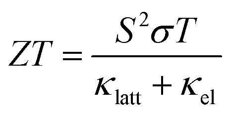 | (1) |
 is the Seebeck coefficient, σ is the electrical conductivity, S2σ is the power factor, and κlatt and κel are the lattice (phonon) and electronic components of the thermal conductivity κ. The electrical properties S, σ and κel are interdependent through the carrier concentration n such that the best ZT are typically found in doped semiconductors,2 and the figure of merit can be tuned to a target operating temperature by chemical doping. In most high-performance TEs the electronic thermal conductivity is negligible and thus the κlatt represents the bulk of the denominator. κlatt is independent of n, and most high-performance TEs are materials with large intrinsic phonon anharmonicity and naturally low thermal conductivity. As for the electrical properties, the κlatt can also be tuned to some extent by alloying,9–11 chemical doping12 and hierarchical nanostructuring.13
Commercial TEGs are currently based on doped Bi2Te3, which shows a ZT of ∼1 at room temperature corresponding to a 2–3% heat recovery.1 PbTe is also a well-established standard for high-temperature TEGs,14 and endotaxial nanostructuring with SrTe has been shown to yield a ZT > 2 above 800 K.13 However, both materials are unsuitable for widespread application for a number of reasons, chief among them the low natural abundance of Te and the environmental toxicity of Pb.1 This has prompted interest in a range of alternative material systems including oxides and other chalcogenides,15 half-Heuslers,16 Zintl compounds,17 and “phonon-glass electron-crystal” framework materials such as clathrates18 and skutterudites.19
Reports of a high-temperature ZT up to 2.6 in SnSe20,21 have led to considerable interest in this system for thermoelectric applications. Despite its relatively simple structure and the low atomic masses of its constituent atoms, SnSe has unusually low thermal conductivity due to the strongly-anharmonic lattice dynamics associated with its high-temperature Pnma-to-Cmcm phase transition.22–24 However, despite a low κlatt and similar anharmonic lattice dynamics,25,26 the isostructural SnS has much lower performance than SnSe.27,28 Various studies have therefore looked at Sn(S,Se) alloys and reported that the ZT is optimised for 80–85% Se content, due in part to a reduction in the κlatt.9–11
Since the terms in eqn (1) are amenable to calculation, first-principles modelling e.g. with density-functional theory has played an instrumental role in our current understanding of the material features that favour high thermoelectric performance. In particular, it has recently become feasible to accurately model lattice dynamics29 and thermal transport,30–32 and insight from studying highly-anharmonic materials is helping to establish structure/property relationships for identifying new high-performance TEs and optimising the performance of existing materials.23,24,33,34 More recently, high-throughput modelling studies have been applied to identify potentially promising but previously-overlooked TEs from known materials.35–37 However, the inherent difficulty of modelling solid solutions means that comparatively little modelling work has been done to understand the impact of alloying on thermoelectric properties.
In our previous work, we developed first-principles models for four Snn(S1−xSex)m solid solutions and investigated the effect of alloying on the optoelectronic properties.38 This was subsequently extended to investigate the effect of alloying on the lattice dynamics of the Pnma Sn(S1−xSex) system and to obtain qualitative insight into the impact of alloying on the thermal transport.39 In this work, we extend these studies to quantify the thermal transport in the Se-rich Sn(S0.1875Se0.8125) alloy. Using analysis techniques developed in our previous work,34 we show that the difference in the κlatt of the SnS and SnSe endpoints is a balance of reduced phonon group velocities and longer lifetimes. We find that Sn(S0.1875Se0.8125) shows near-ideal mixing behaviour, with the mixing free energy dominated by entropy and a near-homogenous distribution of chalcogen atoms over the lattice sites. We investigate several models for calculating the thermal transport of the solid solution and demonstrate that alloying reduces the κlatt by 40–60% compared to SnSe, due to a large reduction in the group velocity of the heat-carrying modes and a small secondary reduction in the phonon lifetimes. These results lay a foundation for future theoretical studies to improve our fundamental understanding of the impact of alloying on lattice thermal conductivity, and thereby design new high-performance alloys for future thermoelectric applications.
2. Methods
The starting point for this work was our previous calculations on the Pnma Sn(S1−xSex) alloy system.38,39 The alloy model is based on a 32-atom 2 × 1 × 2 supercell of the eight-atom Pnma unit cell, which has 2446 unique configurations in 17 compositions between the x = 0 (SnS) and x = 1 (SnSe) endpoints. A set of optimised structures and lattice energies were taken from the dataset published with ref. 38 (ref. 40) and new phonon and thermal-transport calculations were performed on the SnS and SnSe endpoints together with the 23 unique structures with composition x = 0.8125 (i.e. Sn(S0.1875Se0.8125)). We note that this composition was not included in our previous study on the structural dynamics of the Pnma Sn(S1−xSex) system.39Our calculations were performed using periodic pseudopotential plane-wave density-functional theory (DFT) as implemented in the Vienna Ab initio Simulation Package (VASP) code.41 The technical parameters used were as in our previous work.38,39 The PBEsol functional42 with the DFT-D3 dispersion correction43 (i.e. PBE+D3) was used to model electron exchange and correlation. A plane-wave basis with a 600 eV kinetic-energy cutoff and a 4 × 4 × 4 Monkhorst–Pack k-point sampling mesh44 were used to represent the electronic structure of the alloy supercell. Projector augmented-wave (PAW) pseudopotentials45,46 were used to treat the core electrons, with the Sn 5s, 5p and 4d, the S 3s and 3p, and the Se 4s and 4p electrons in the valence region. The electronic wavefunctions were optimised to a tight tolerance of 10−8 eV on the total energy. The precision of the charge-density grids was set automatically to avoid aliasing errors, and a support grid with 8 × the number of points was used to evaluate the augmentation chares. The PAW projection was performed in reciprocal space, and non-spherical contributions to the gradient corrections inside the PAW spheres were accounted for. These settings minimise the numerical noise in the forces, which is required to compute accurate force constants.
Lattice-dynamics and thermal-conductivity calculations were carried out using the Phonopy29 and Phono3py31 codes with VASP as the force calculator. The second- and third-order interatomic force constants were computed using the supercell finite-displacement approach with step sizes of 10−2 and 3 × 10⁻² Å respectively. 2 × 2 × 2 supercells of the 32-atom alloy cells (256 atoms) were used to calculate the second-order interatomic force constants (IFCs), while the single alloy cells were used to compute the third-order IFCs. These are equivalent respectively to 4 × 2 × 4 and 2 × 1 × 2 supercells of the eight-atom Pnma unit cell. Explicit testing showed that with this setup the calculated 300 K κlatt of SnS and SnSe are both converged to within 6% of the values obtained using larger 3 × 2 × 3 and 2 × 1 × 2 second- and third-order expansions of the alloy cell, with 576 and 128 atoms. The k-point meshes used for the alloy cells were reduced proportionally for the supercell calculations.
Phonon density of states (DoS) curves were computed by interpolating the phonon frequencies onto uniform Γ-centered q-point meshes with 16 × 8 × 16 and 8 × 8 × 8 subdivisions for the primitive and alloy supercells respectively. The DoS curves were generated using a Gaussian smearing with a width σ = 0.032 THz, corresponding to a full-width at half-maximum of 2.5 cm−1. To calculate the vibrational contributions to the free energy, phonon frequencies were computed on denser 32 × 16 × 32 or 16 × 16 × 16 grids. Dispersions of Pnma SnS and SnSe were obtained by interpolating frequencies along a path passing through all the high-symmetry wavevectors in the Pnma Brillouin zone. Dispersions of the alloy model were computed by using the band-unfolding algorithm in ref. 47 to project the dispersions back to the Pnma primitive cell. To compute the thermal conductivity, the modal properties were computed on the same grids as used for the DoS, which were found by testing to be sufficient to converge the 300 K κlatt of SnS and SnSe to within 1% of the values obtained using denser 24 × 12 × 24 meshes with ∼3 × as many mesh points. In these calculations, the linear tetrahedron method was used for the Brillouin zone integration.
3. Results and discussion
a. Structure and lattice dynamics of SnS and SnSe
The orthorhombic Pnma structure (Fig. 1) is the ground state phase of SnS and SnSe under ambient conditions.48,49 The Sn(II) oxidation state favours a distorted tetrahedral coordination environment in which each Sn atom forms three bonds to chalcogen atoms and the fourth coordination site is occupied by a steteochemically-active 5s2 lone pair of electrons. This results in a layered structure composed of 2D sheets held together with dispersion interactions facilitated by the Sn lone pairs projecting into the interlayer spacing. The layers stack along the long crystallographic axis (here the b direction), with stronger but anisotropic covalent bonding along the perpendicular in-plane (a/c) directions.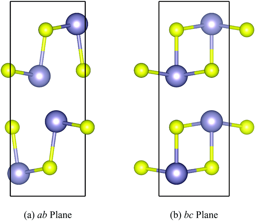 | ||
| Fig. 1 Structure of Pnma SnS shown through the ab (a) and bc (b) planes, illustrating the layering along the b axis and the anisotropic chemical bonding along the perpendicular in-plane a and c axes. S and Sn atoms are shown in yellow and grey, respectively. These images were prepared using the VESTA software (ref. 50). | ||
The optimised lattice constants of the two models are listed and compared to experimental neutron-scattering measurements51 in Table 1. As found in our previous work, the PBEsol+D3 functional gives a good description of the structure, with lattice constants and cell volumes within 0.4–2.7% and ∼4.5% of the experimental measurements. The calculations parameters are technically athermal (0 K) values, whereas the experimental structures were collected at 295 K and are therefore expected to include some degree of thermal expansion, so we consider these discrepancies to be reasonable.
| Expt. | Calc. (this work) | |||||||
|---|---|---|---|---|---|---|---|---|
| a [Å] | b [Å] | c [Å] | V [Å3] | a [Å] | b [Å] | c [Å] | V [Å3] | |
| SnS | 4.336 | 11.143 | 3.971 | 192 | 4.218 (−2.7%) | 10.974 (−1.5%) | 3.957 (−0.35%) | 183 (−4.5%) |
| SnSe | 4.445 | 11.501 | 4.153 | 212 | 4.342 (−2.3%) | 11.338 (−1.4%) | 4.121 (−0.77%) | 203 (−4.4%) |
The calculated phonon dispersion and density of states (DoS) curves of SnS and SnSe are shown in Fig. 2. The eight atoms in the Pnma primitive cell result in 3na = 24 phonon bands at each wavevector q. The phonon spectra of SnS and SnSe can be partitioned into lower-and upper-frequency regions with equal numbers of modes, which the atom-projected DoS (PDoS) curves indicate can be assigned predominantly to motions of the Sn and chalcogen atoms respectively. These two groups of modes are separated by a so-called “phonon bandgap”, which is more prominent in SnS. Due to the heavier chalcogen and weaker chemical bonding, the phonon spectrum of SnSe spans a smaller frequency range of 0–6 THz compared to the 0–9 THz frequency range of the SnS spectrum. In both systems, the acoustic mode frequencies range from ∼0–1.5 THz and overlap with some of the optic modes in the low-frequency region of the spectrum. Finally, the comparatively flat dispersion along the X–S and R–U segments of the dispersion, which correspond to the b direction in real space, highlights the weaker interlayer interactions along this direction.
 | ||
| Fig. 2 Calculated phonon dispersion and phonon density of states (DoS) curves for SnS (a) and SnSe (b). In each of the DoS plots, the projections onto Sn and S/Se atoms are shown as overlaid blue and red/orange shaded curves. | ||
b. Lattice thermal conductivity of SnS and SnSe
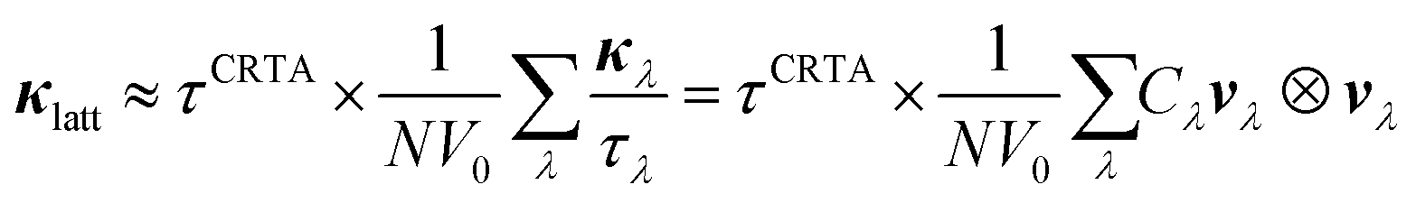
Using the single-mode relaxation-time approximation (RTA) solution to the phonon Boltzmann transport equations, the κlatt is computed according to:31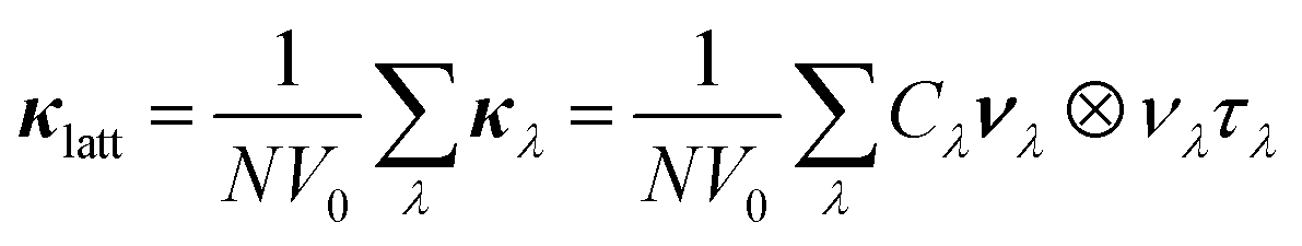 | (2) |
Fig. 3a and b show the calculated κlatt of SnS and SnSe as a function of temperature. The thermal transport of the orthorhombic Pnma structure is anisotropic, so we consider separately the three diagonal elements of the tensor κxx, κyy, and κzz, which correspond to transport along the a, b and c axes respectively, together with the average  . Calculated values at T = 300 K are listed in Table 2.
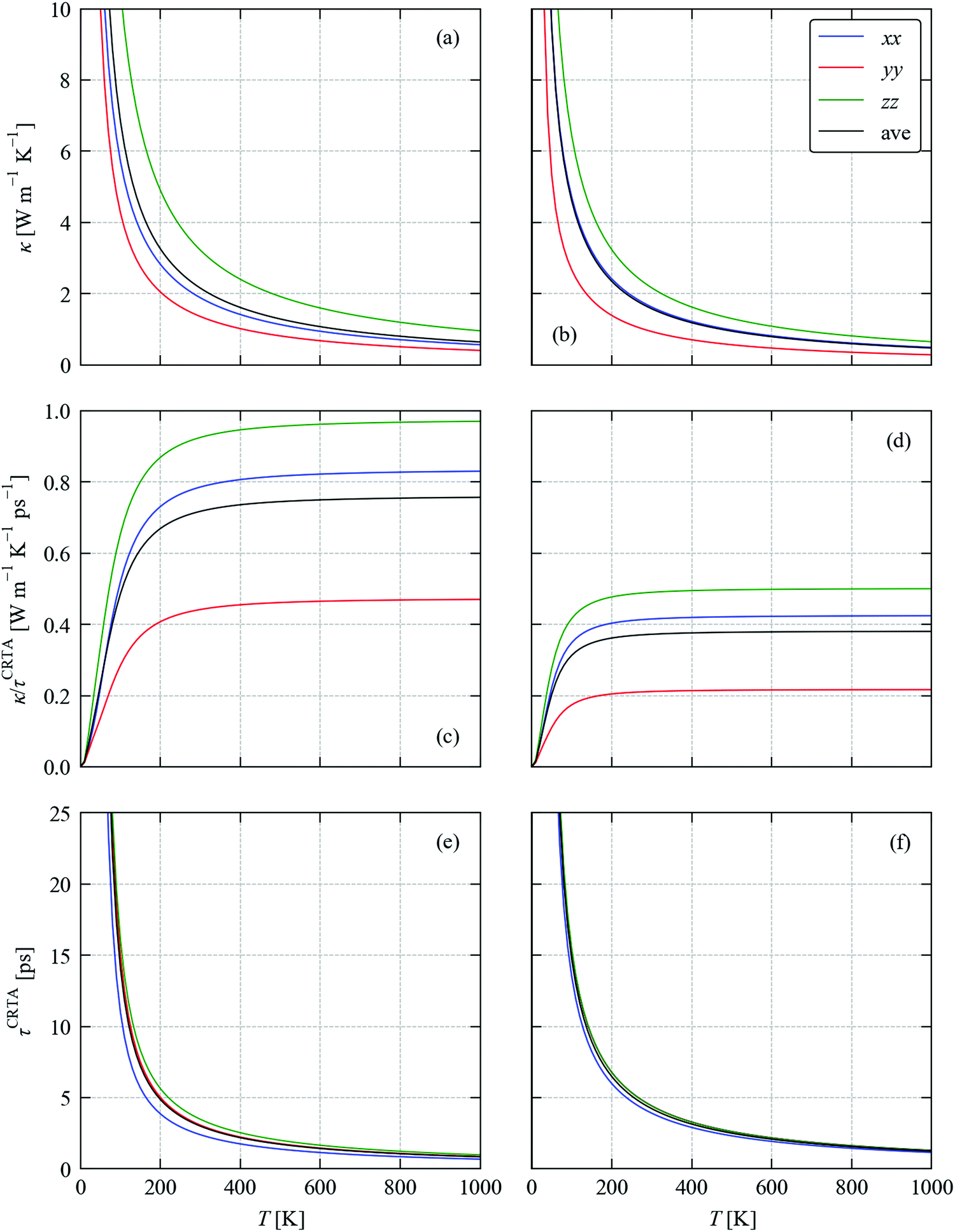 | ||
Fig. 3 Calculated thermal conductivity of SnS (left) and SnSe (right) as a function of temperature analysed using the constant relaxation time approximation (CRTA) model defined in eqn (3) and (4). (a) and (b) Thermal conductivity κlatt. (c) and (d) Harmonic component κlatt/τCRTA. (e) and (f) Lifetime component τCRTA. On each subplot, the tensor components along the a (xx, blue), b (yy, red) and c (zz, green) directions are shown together with the average  (ave, black). (ave, black). | ||
![[small tau, Greek, macron]](https://www.rsc.org/images/entities/i_char_e0d4.gif) λ averaged over all modes for comparison to the τCRTA. Row 5 lists the average phonon–phonon interactions strengths
λ averaged over all modes for comparison to the τCRTA. Row 5 lists the average phonon–phonon interactions strengths ![[P with combining tilde]](https://www.rsc.org/images/entities/i_char_0050_0303.gif) that reproduce the κlatt components when used with the model in eqn (8), and Row 6 lists the interaction strengths
that reproduce the κlatt components when used with the model in eqn (8), and Row 6 lists the interaction strengths ![[P with combining macron]](https://www.rsc.org/images/entities/i_char_0050_0304.gif) λ averaged over all modes, which are again scalar values
λ averaged over all modes, which are again scalar values
| SnS | SnSe | |||||||
|---|---|---|---|---|---|---|---|---|
| xx | yy | zz | ave | xx | yy | zz | ave | |
| κ latt [W m−1 K−1] | 1.88 | 1.36 | 3.22 | 2.15 | 1.62 | 0.94 | 2.16 | 1.58 |
| κ latt/τCRTA [W m−1 K−1 ps−1] | 0.786 | 0.442 | 0.925 | 0.718 | 0.415 | 0.212 | 0.490 | 0.372 |
| τ CRTA [ps] | 2.40 | 3.07 | 3.48 | 3.00 | 3.91 | 4.42 | 4.42 | 4.23 |
|
λ
[ps] |
3.69 | 4.34 | ||||||
|
[10−11 eV2] |
4.87 | 4.60 | 3.99 | 4.37 | 1.92 | 1.98 | 1.85 | 1.90 |
|
λ
[10−11 eV2] |
24.6 | 9.81 | ||||||
For SnS we calculate room-temperature conductivities of 1.88, 1.36 and 3.22 W m−1 K−1 along the crystallographic a, b and c axes, giving an average value of κave = 2.15 W m−1 K−1. In our model, the b and c axes correspond respectively to the layering direction and the direction of strongest in-plane bonding (cf.Fig. 1), and thus have the smallest and largest κlatt. We note that these values are considerably higher than in our previous calculations,52 where we obtained values of κxx = 0.74, κyy = 0.36, κzz = 1.10 and κave = 0.73 W m−1 K−1. This discrepancy can be attributed to differences in the supercells used to compute the second- and third-order force constants, to the inclusion of the DFT-D3 dispersion correction in the present calculations, and also to some convergence issues in the previous calculations. From a technical perspective, we expect the present results to be more accurate.
For SnSe we calculate room-temperature conductivities of 1.62, 0.94 and 2.16 W m−1 K−1 along the a, b and c axes and an average of 1.58 W m−1 K−1. As for SnS, the κlatt is strongly anisotropic with the smallest and largest components along the b and c axes respectively. These are also larger than, albeit similar to, the values we obtained in our previous calculations,23viz. 1.44, 0.53 and 1.88 W m−1 K−1 along the three axes and an average of 1.28 W m−1 K−1. This discrepancy can again be attributed to differences in the technical parameters used in the two sets of calculations. The dispersion correction reduces the lattice constants and cell volume by ∼0.7 and 2.1%, respectively, and is likely to result in stronger non-bonded interactions along the b axis where the discrepancy with previous calculations is largest. As for SnS, we again expect the present results to be technically more accurate.
Ref. 20 reports single-crystal κlatt measurements on SnSe of 0.67, 0.46 and 0.70 W m−1 K−1 along the equivalent directions to the a, b and c axes in our calculations. It was subsequently noted however that that the density of these crystals was ∼10% lower than the expected theoretical value.53 The aggregated room-temperature κlatt measurements in ref. 53 span a range of ∼0.7–1.4 W m−1 K−1 along the in-plane a and c directions and ∼0.5–0.9 W m−1 K−1 along the layered b axis. This ∼2 × spread in measured results clearly highlights the sensitivity of the κlatt to the material preparation and handling. However, the upper range of these values are reasonably comparable to our calculations. Possible origins of the discrepancy between different measurements are a typical 15–20% error in measurements of the thermal diffusivity,21 the presence of vacancies and interstitials,53 microcracks caused by the high-temperature phase transition,54 and oxidation at high temperatures.55 It is also likely that the RTA calculations we perform here will overestimate the κlatt to some extent due to a neglect of thermal expansion at finite temperature, higher-order (e.g. 4th order) phonon–phonon interactions,56 and non-perturbative anharmonicity associated with the high-temperature phase transition.22–24
We were unable to find any reports of single-crystal κlatt measurements on SnS. Ref. 10,27 report polycrystalline values of ∼1.25 and 1.15–1.30 W m−1 K−1 at 300 K, which are again lower than but reasonably comparable to our calculations. It is of course likely that the two sets of experimental measurements would be subject to the same issues as measurements on SnSe. In the same vein, SnS also shows a high-temperature Pnma → Cmcm phase transition and the same non-perturbative anharmonicity as SnSe,26,48 which may result in our calculations overestimating the κlatt.
The effect of grain boundaries in polycrystalline samples (or present as defects in single crystals) can be investigated using a simple boundary-scattering model to limit the mean-free paths of the long-wavelength phonon modes (see ESI†). We find that the lower range of experimental values on SnSe can be recovered by imposing a boundary limit of ∼10 nm, while a κave comparable to measurements on SnS can be recovered with a limit of around 10–20 nm.
To investigate the difference in the κlatt of SnS and SnSe, we used the constant relaxation-time approximation (CRTA) model developed in ref. 34 in which the τλ are replaced with a constant τCRTA such that the κlatt can be written:
 | (3) |
We further modify eqn (3) to replace the scalar τCRTA with a tensor so that individual components of κlatt are computed as follows:
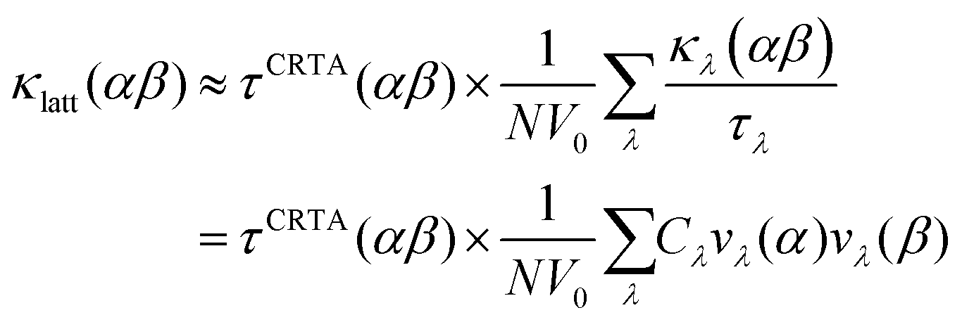 | (4) |
The temperature dependence of the harmonic component κlatt/τCRTA on the right-hand side of eqn (3) and (4) and the lifetime component τCRTA are shown in Fig. 3c, d and e, f respectively. This analysis clearly shows that the harmonic term is much smaller in SnSe than SnS, which can be attributed to the weaker bonding and heavier chalcogen and hence lower group velocities. Interestingly, this is offset by longer τCRTA in SnSe. Comparing the values at T = 300 K (Table 2) shows the harmonic terms along the three principal directions are reduced by 47–52% in SnSe while the lifetimes are increased by 27–63%, which leads to an overall decrease of 14–33% in the κlatt components. We made a similar qualitative conclusion in our previous work39 based on data from previous calculations.23,52 Although the longer τCRTA in SnSe indicate it to be less anharmonic than SnS, the τCRTA in both are on the order of ps and are very short in comparison to other systems – for example, a similar CRTA analysis on CoSb3 yields an order-of-magnitude larger τCRTA of 36.6 ps.34Fig. 3c and d also show that the anisotropy in the thermal transport is again largely due to differences in the harmonic term, as there is a 2.1–2.3 × variation in the κlatt/τCRTA but a much smaller 1.1–1.5 × variation in the τCRTA. This confirms that the anisotropy in the chemical bonding has a large effect on the group velocities and hence the thermal transport.
We note that a similar constant relaxation-time model is often used to model the electronic transport properties of thermoelectric materials (as implemented in e.g. the BoltzTraP code57), but there are few if any examples of its application to modelling lattice thermal conductivity. However, a key difference is that whereas the relaxation time in electronic transport calculations is often assumed to be independent of temperature and energy, in the present model the τCRTA are independent of energy (i.e. phonon frequency) but not temperature. Comparison of Fig. 3a, b and e, f clearly shows that the temperature dependence of the κlatt is strongly linked to the temperature dependence of the phonon lifetimes, particularly above the Dulong–Petit limit where the Cλ and hence the κlatt/τCRTA saturate, and thus a temperature-dependent τCRTA is required for this model to be reasonable.
While the origin of the differences in the harmonic components κlatt/τCRTA can be understood by the differences in chalcogen mass and chemical bonding, the origin of the longer phonon lifetimes in SnSe require further investigation. As outlined in ref. 31, the lifetimes are computed from the inverse of the phonon linewidths Γλ according to:
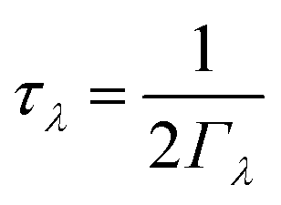 | (5) |
The Γλ are computed as a sum of contributions from three-phonon interactions using the expression:
 | (6) |
 | (7) |
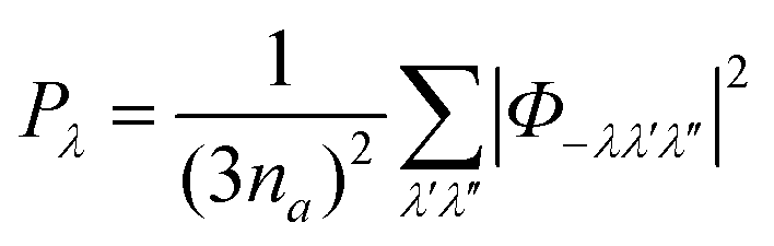
Following ref. 31, an approximate linewidth Γλ can be written as:
 | (8) |
 | (9) |
| N2(q,ω) = N(1)2(q,ω) + N(2)2(q,ω) | (10) |
The N2(q, ω) is the sum of separate functions for collision (Type 1) and decay (Type 2) events:
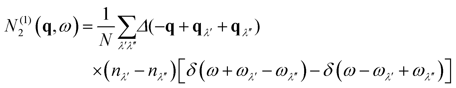 | (11) |
 | (12) |
Collisions correspond to phonon absorption through the coalescence of two modes, i.e. λ + λ′ → λ′′ or λ + λ′′ → λ′, while decay processes correspond to emission, i.e. λ → λ′ + λ′′. For comparing between materials it is convenient to average the N2(q,ω) over wavevectors to obtain a function of frequency only, which we denote ![[N with combining macron]](https://www.rsc.org/images/entities/i_char_004e_0304.gif) 2(ω) with corresponding components (1)2(ω) and (2)2(ω):
2(ω) with corresponding components (1)2(ω) and (2)2(ω):
 | (13) |
Fig. 4a, b and c, d compare respectively the 2(ω) and spectra of Pλ for SnS and SnSe. At frequencies below ∼2 Thz in both systems there are very few decay (emission) pathways and the phonon scattering is dominated by collisions (absorption). At higher frequencies, decay pathways become available and become the dominant scattering mechanism from around 3 THz. Across most of the frequency spectrum the 2(ω) are 1.5–2× higher in SnSe than in SnS, indicating that the smaller range of frequencies in the former leads to a higher density of energy-conserving scattering pathways. The Pλ of SnS and SnSe both form two clear groups, spanning a range of 10−11–10−10 eV2 at low frequency and 10−10–10−9 eV2 at high frequency, indicating that the high-frequency modes interact an order of magnitude more strongly with other phonons than the low-frequency modes. This analysis also clearly shows that the phonon–phonon interaction strengths for both groups of modes are considerably weaker in SnSe than in SnS. Given the longer τCRTA in SnSe, the weaker Pλ therefore counteract the larger 2(ω) and lead to longer lifetimes, at least for the dominant heat-carrying modes, This analysis is again in line with our previous work.39
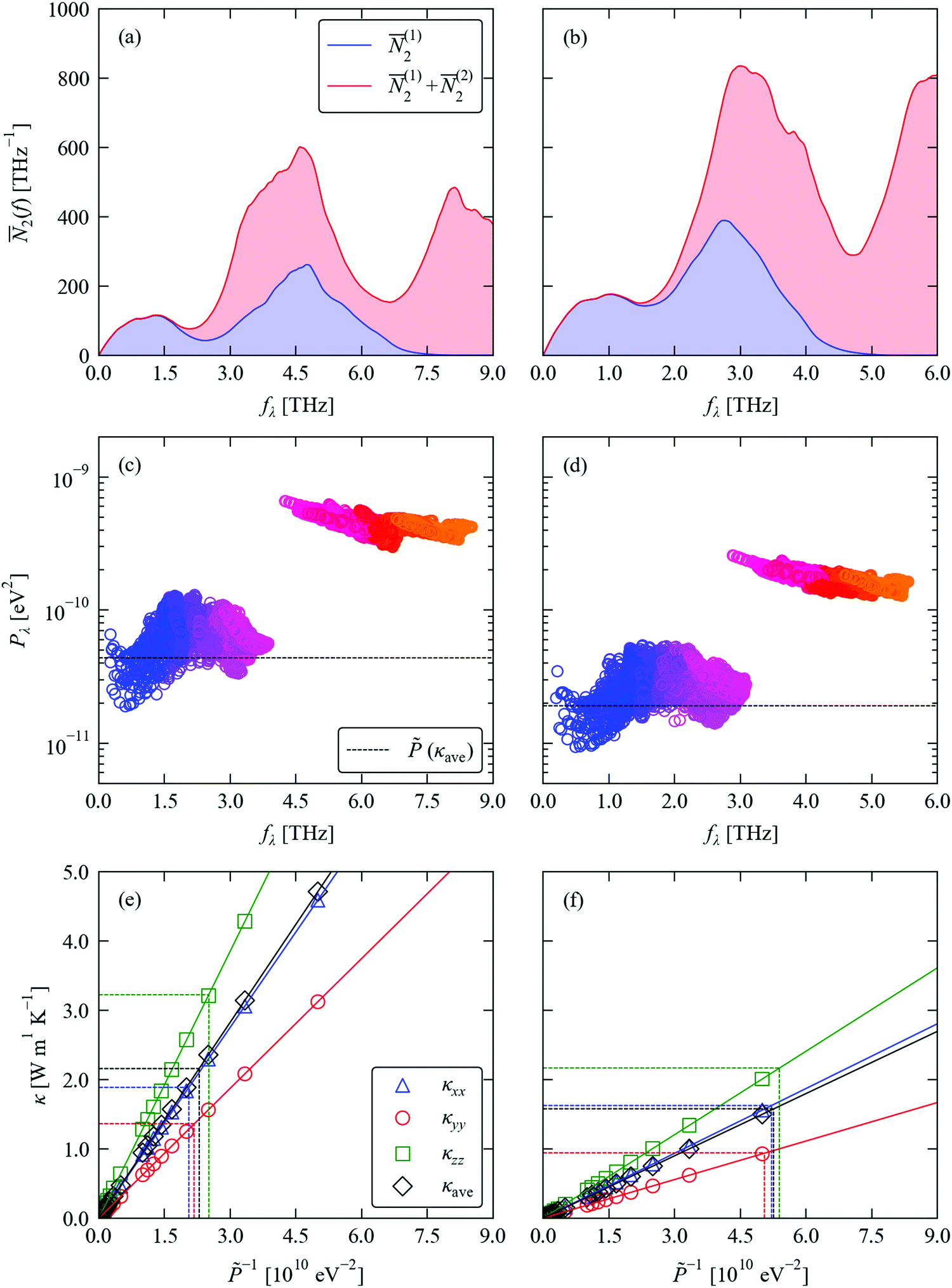 | ||
| Fig. 4 Analysis of the phonon lifetimes/linewidths in SnS (left) and SnSe (right). (a) and (b) Two-phonon weighted join density-of-states (w-JDoS) functions 2(ω) defined in eqn (13). (c) and (d) Spectra of modal phonon–phonon interaction strengths Pλ defined in eqn (9). The constant phonon–phonon interaction strengths that reproduce the average thermal conductivity κave at T = 300 K are indicated by dashed black lines. (e) and (f) Dependence of the principal thermal conductivity components κxx/κyy/κzz and κave at 300 K on the averaged phonon–phonon interaction strength . The values of that reproduce the calculated κxx, κyy and κzz and κave are indicated by dashed lines. | ||
We previously demonstrated that finding a constant value such that replacing the Pλ in eqn (8) reproduces the κlatt provides a useful metric for comparing the relative phonon–phonon interaction strengths in different materials.34 From the relationships in eqn (2), (5) and (8), the κlatt is inversely proportional to , and a suitable value can be estimated from a simple linear fit (Fig. 4e, f and Table 2). For SnS and SnSe, we obtain values of 3.99–4.87 × 10¹¹ and 1.85–1.98 × 10¹¹ eV2, respectively. These are heavily weighted toward the Pλ of the lower-frequency modes (cf.Fig. 4c and d), which can be understood from the fact that the majority of the heat transport in semiconductors is typically through acoustic and low-lying optic modes. This analysis thus reaffirms that the phonon–phonon interactions in SnSe are weaker than in SnS.
Overall, our calculations indicate that the κlatt of SnS and SnSe are similar and both ultra-low. A comparison of the room-temperature κlatt of SnS and SnSe using the CRTA model shows that SnSe has lower group velocities but longer lifetimes than SnS, resulting in an overall decrease in the thermal transport of 14, 31 and 33% along the a, b and c directions, respectively. Considering the w-JDoS and Pλ/ we can further attribute the differences in lifetimes to the larger number of energy-conserving scattering pathways enabled by the smaller range of phonon frequencies in the SnSe spectrum being counteracted by weaker phonon–phonon interaction strengths. The fact that SnS and SnSe have similar κlatt and that the difference arises from a balance of two opposing effects means it would not be entirely unexpected if the qualitative ordering was sensitive to the theoretical methodology employed. Certainly, the spread in experimental measurements highlighted for SnSe in ref. 53 suggests that it is difficult to make a conclusive ordering on the basis of experiments alone.
c. Statistical thermodynamics of the Sn(S0.1875Se0.8125) solid solution
We previously developed a structural model for the Pnma Sn(S1−xSex) alloy following the approach in ref. 58.38 The model comprises a set of 17 compositions between the SnS (x = 0) and SnSe (x = 1) endpoints, where each composition is a set of nx symmetry-inequivalent chalcogen arrangements in a 32-atom 2 × 1 × 2 supercell expansion of the eight-atom Pnma unit cell. In this work, we examine the Sn(S0.1875Se0.8125) composition (i.e. x = 0.8125), for which there are nx = 23 independent configurations. This is a manageable number for performing accurate phonon calculations, and the composition is within the 80–85% Se range where the κlatt is reported to reach a minimum.9–11For each of the structures we calculate a lattice internal energy Ulatt, which we equate to the DFT total energy E, and a temperature-dependent constant-volume (Helmholtz) free energy A(T) including contributions from the phonons:
| Ai(T) =Ulatti + Avibi(T) = Ulatti + Uvibi(T) − TSvibi(T) | (14) |
 | (15) |
 | (16) |
Given the lattice internal or Helmholtz energies for each of the nx structures for composition x, analogous thermodynamic partition functions Z(x;T) and free energies A(x;T) can be computed as:
 | (17) |
A(x;T) = −kBT![[thin space (1/6-em)]](https://www.rsc.org/images/entities/i_char_2009.gif) ln ln![[thin space (1/6-em)]](https://www.rsc.org/images/entities/char_2009.gif) Z(x;T) = Ūlatt(x;T) − TSconf(x;T) Z(x;T) = Ūlatt(x;T) − TSconf(x;T) | (18) |
 | (19) |
A(x;T) = −kBTlnZ(x;T) = Ā(x;T) − TSconf(x;T) = Ūlatt(x;T) + Ūvib(x;T) − T[![[S with combining macron]](https://www.rsc.org/images/entities/i_char_0053_0304.gif) vib(x;T) + Sconf(x;T)] vib(x;T) + Sconf(x;T)] | (20) |
In these expressions, the degeneracies gi are the number of alternative chalcogen arrangements that are equivalent under the symmetry operations of the parent Pnma structure, Ūlatt/Ā are the weighted average lattice/Helmholtz energies of the structures for the composition x, and Sconf is the vibrational entropy.
Once the A(x;T) has been calculated, a mixing free energy Amix(x;T) can be computed with reference to the free energies of the endpoints A(x = 0;T) and A(x = 1;T) according to:
| Amix(x;T) = A(x;T) − [(1 − x)A(x = 0;T) + xA(x = 1;T)] | (21) |
Given a Z(x;T), the occurrence probabilities Pi of each of the nx structures can also be computed from:
 | (22) |
 | (23) |
These weights can then be used to compute the thermodynamic average ![[X with combining macron]](https://www.rsc.org/images/entities/i_char_0058_0304.gif) of a general physical property X as:
of a general physical property X as:
 | (24) |
For example, the Ūlatt and Ā in eqn (18) and (19) are computed by averaging the Ulatti and Ai using eqn 24 and the appropriate Pi from eqn (22) or (23). It is typically assumed that the distribution of configurations is kinetically trapped when the alloy is formed, and the Pi are therefore computed at the formation temperature TF.58 In our previous work, we used a value of TF = 900 K.38,39
We previously compared the Amix(x;T) and Pi(x;T) obtained using the Ulatti and Ai(T) for several compositions of the Sn(S1−xSex) alloy and found that differences in phonon frequencies both disfavoured the mixing (i.e. predicted more positive Amix) and resulted in substantially different distributions of occurrence probabilities.39 However, the Avibi were determined from force constants obtained in the 32-atom alloy supercells, as the number of configurations made this a necessary approximation. Given that a larger 256-atom supercell expansion is required to converge the κlatt of the endpoints, we investigated the extent to which the supercell used to compute the force constants influences the free energies.
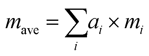
Fig. 5a compares the calculated mixing energy of Sn(S0.1875Se0.8125) as a function of temperature based on A(x;T) computed from the lattice energies and Helmholtz energies with phonon frequencies obtained using the 32-atom alloy supercells and 256-atom expansions. We find that the Helmholtz energies calculated using the larger supercell yield very similar mixing energies to the lattice energies, whereas the Helmholtz energies calculated using the alloy supercell result in a very different temperature dependence.
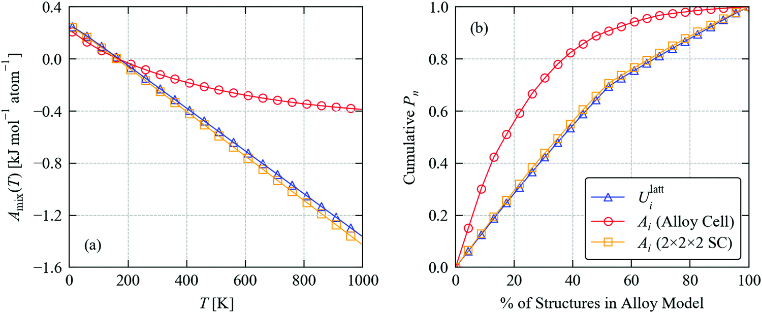 | ||
| Fig. 5 Thermodynamics of the Sn(S0.1875Se0.8125) solid solution: (a) mixing free energy Amix as a function of temperature computed from eqn (21); and (b) cumulative distribution of occurrence probabilities Pi as a function of the percentage of structures in the alloy model at a formation temperature TF = 900 K computed using eqn (22) and (23). Each plot compares calculations using the lattice energies Ulatti and the constant–volume (Helmholtz) free energies Ai(T), which include vibrational contributions to the internal energy and entropy calculated using force constants obtained with the 32-atom alloy supercells and 256-atom supercell expansions. | ||
For the SnS and SnSe endpoints, calculations using the 32-atom alloy supercell underestimate the 900 K Avib by 0.3 and 0.15 kJ mol−1 atom−1, respectively, compared to larger 256-atom supercells. Among the 23 configurations in the alloy model, the range of Ulatti is 0.07 kJ mol−1 atom−1, whereas the ranges in the Avibi computed using the small and large supercell are 1.13 and 0.06 kJ mol−1 atom−1 respectively. This suggests the error associated with the small supercell is even larger for structures in the mixed-composition model.
We also compared the individual contributions to the mixing free energy at TF = 900 K from the lattice and vibrational internal energy, Ulattmix/Uvibmix, and from the configurational and vibrational entropy, Sconfigmix/Svibmix (Table 3). Using the Ulatti, the Ulattmix and −TSconfigmix terms are 0.28 and −1.48 kJ mol−1 atom−1, respectively, and the small increase in internal energy is compensated by the much larger configurational entropy to produce an overall negative Amix of −1.20 kJ mol−1 atom−1. Using the Ai from the smaller alloy supercell predicts that differences in the Uvibmix and Svibmix combine to disfavour the mixing by 0.64 kJ mol−1 atom−1, while the contribution from configurational entropy is also reduced by around 13% presumably due to the more skewed distribution of Pi in Fig. 5b. Together, these result in a much less negative predicted Amix of −0.37 kJ mol−1 atom−1. On the other hand, when the Ai are computed using the larger phonon supercell expansions, the Pi and thus the Sconfigmix are very close to the result obtained using the lattice energies, and the vibrational contributions to the mixing are very small, with differences in vibrational entropy favouring mixing by an additional 0.06 kJ mol−1 atom−1.
| [kJ mol−1 atom−1] | U latt i | A i | |
|---|---|---|---|
| Alloy cell | 2 × 2 × 2 SC | ||
| A mix | −1.20 | −0.37 | −1.26 |
| U mix | 0.28 | −0.18 | 0.28 |
| −TSmix | −1.48 | −0.19 | −1.53 |
| U lattmix | 0.28 | 0.28 | 0.28 |
| U vibmix | — | −0.46 | 0.00 |
| −TSvibmix | — | 1.09 | −0.06 |
| −TSconfigmix | −1.48 | −1.29 | −1.48 |
The clear implication of this result is that the force constants obtained using the 32-atom alloy supercell do not yield sufficiently accurate frequencies to compute accurate Helmholtz energies. As a result, our previous conclusion that differences in vibrational frequencies disfavour the mixing and skew the distribution of occurrence probabilities in the Pnma Sn(S1−xSex) alloy may not be correct. Indeed, the present finding suggests that it is not necessary to consider the phonon contributions to the free energy in order to obtain a reasonable thermodynamic model for this system. However, we previously found that the full range of Snm(S1−xSex)n systems form near-ideal solid solutions, based on alloy models using the lattice energies, and it is entirely possible the lattice dynamics would have a more significant impact on the thermodynamics of less ideal systems. Either way, our findings clearly highlight the need carefully to check the convergence of the free energies with respect to the accuracy of the force constants.
d. Thermal conductivity of Sn(S0.1875Se0.8125)
We now consider the thermal conductivity of the Sn(S0.1875Se0.8125) alloy model. Fig. 6 shows the unfolded dispersion and atom-projected DoS of Sn(S0.1875Se0.8125), computed as a thermodynamic average using eqn (24) at a formation temperature TF = 900 K. | ||
| Fig. 6 Unfolded dispersion and atom-projected density of states (PDoS) of Sn(S0.1875Se0.8125). The colour scale in the unfolded dispersion represents the spectral weight and runs from blue (low weight) to yellow (high weight). | ||
The PDoS is similar to that of SnSe but with an additional feature above ∼6 THz comprising modes predominantly associated with S vibrations. The lower-frequency part of the unfolded dispersion, which consists predominantly of Sn-based modes, retains considerable structure, albeit with some smearing, suggesting that the Sn sublattice is largely unaffected by the alloying. On the other hand, the mid-frequency Se-based bands show considerably more broadening, and the dispersion of the high-frequency S bands has very little structure. Since the low-frequency modes are the dominant heat carriers, and the corresponding part of the dispersion remains similar to SnSe, it is not clear from this analysis to what extent the alloying will affect the thermal conductivity through changes to the group velocities.
We also note that, unlike in our previous work, we see no evidence of imaginary modes in the unfolded dispersion, which we also confirmed by inspecting of the phonon frequencies at the commensurate wavevectors for each of the alloy configurations. This again highlights the importance of using a sufficiently large supercell for computing the force constants.
Since Sn(S0.1875Se0.8125) is close to the SnSe endpoint, a very simple reference point for the κlatt is to use the SnSe force constants and adjust the mass of the chalcogen atoms to a weighted average:
 | (25) |
 | (26) |
We previously used this technique to investigate the thermal conductivity of the Li(Ni,Mn,Co)O2 (NMC) alloy system.60
Fig. 7 compares the κlatt obtained from this model with the thermal conductivity of SnSe computed in the alloy supercell, the latter of which gives a thermal conductivity within 5% of the value computed using the primitive cell. Instead of considering transport along the a, b, and c directions separately, as we did for the endpoints, we discuss the in-plane and out-of-plane thermal conductivity perpendicular and parallel to the layering direction, respectively, which we denote  and κ‖ = κyy, as well as the average
  . This is because we would not necessarily expect the bonding anisotropy along the a and c axes to be retained in the alloy models.
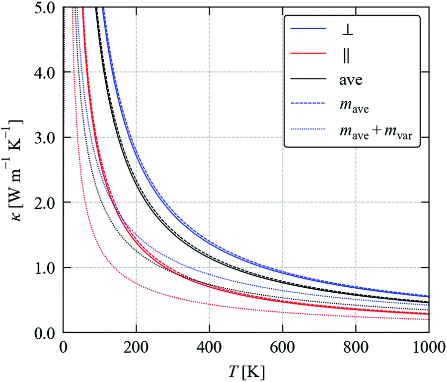 | ||
| Fig. 7 Impact of mass variation at the chalcogen site in SnSe on the thermal conductivity κlatt. The solid lines show the in-plane (κ⊥, blue), out-of-plane (κ‖, red) and average κlatt (κave, black) of SnSe. The corresponding values obtained by changing the average mass mave at the chalcogen site to mimic the Sn(S0.1875Se0.8125) solid solution are shown by dashed lines, and the values obtained by additionally including isotope scattering due to the change in mass variance mvar are shown by dotted lines. | ||
Decreasing the average mass to mave = 0.1875mS + 0.8125mSe predicts a ∼2–4% increase in the κlatt compared to SnSe. This is readily understood given the larger group velocities in SnS (cf.Fig. 3). Including the isotope scattering, on the other hand, predicts a surprisingly large 40% reduction in the κlatt of the alloy, with the κ⊥, κ‖ and κave reduced from 1.82, 0.93 and 1.53 W m−1 K−1 in SnSe to 1.11, 0.55 and 0.93 W m−1 K−1 at T = 300 K (Table 4). The isotope scattering model in ref. 59 is usually used to model the effect of natural isotope variation on the κlatt. For Sn, S and Se, the natural mvar computed using eqn (26) are 3.34, 1.65 and 4.63 × 10⁻⁴, respectively, and we previously found that isotope scattering has very little effect on the thermal conductivity of SnS.25 On the other hand, the mvar parameter computed for Sn(S0.1875Se0.8125) is 6.85 × 10⁻², i.e. two orders of magnitude larger (Table 4).
| Sn(S0.1875Se0.8125) | SnSe | ||||||
|---|---|---|---|---|---|---|---|
| ⊥ | ‖ | ave | ⊥ | ‖ | ave | ||
| Mass Var. | m ave [amu] | 70.2 | 79.0 | ||||
| m var | 6.85 × 10⁻² | — | |||||
| κ latt [W m−1 K−1] | 1.11 | 0.55 | 0.93 | 1.82 | 0.93 | 1.53 | |
| CRTA | κ latt/τCRTA [W m−1 K−1 ps−1] | 0.215 ± 0.014 | 0.088 ± 0.005 | 0.173 ± 0.010 | 0.433 | 0.212 | 0.360 |
| τ CRTA [ps] | 3.96 | 4.17 | 4.03 | 4.18 | 4.41 | 4.24 | |
| κ latt [W m−1 K−1] | 0.85 ± 0.06 | 0.37 ± 0.02 | 0.70 ± 0.04 | 1.82 | 0.93 | 1.53 | |
| Const. |
[10−12 eV2] |
1.47 | 1.17 | 1.24 | 1.18 | ||
| κ latt [W m−1 K−1] | 0.73 ± 0.03 | 0.39 ± 0.01 | 0.62 ± 0.02 | 1.82 | 0.93 | 1.53 | |
To obtain the calculated κlatt in Fig. 3 required a total of 16 accurate force calculations on 256-atom cells and 2580 calculations on 32-atom cells to obtain the second- and third-order force constants, respectively, using the supercell finite-displacement method. For the 23 configurations in our Sn(S0.1875Se0.8125) model, obtaining the second-order force constants required 3536 calculations on 256-atom cells, which was challenging but possible. To obtain the third-order force constants, however, would require 649096 calculations on 32-atom cells, which is not feasible.
Returning to the CRTA model defined in eqn (3) and (4), we can use the second-order force constants to compute an averaged κlatt/τCRTA for the alloy and thereby quantify the impact of changes to the frequencies and group velocities on the κlatt. As shown in Fig. 8a and b, the alloying is predicted to reduce the harmonic term by 2–2.5× compared to SnSe, with the in-plane and out-of-plane values falling from 0.433 and 0.212 to 0.215 and 0.088 W m−1 K−1 ps−1 at T = 300 K (Table 4). The estimates of the spread of values, given by the weighted standard deviations, are on the order of 5%. If we assume that the lifetime term τCRTA can be interpolated between the SnS and SnSe endpoints, we obtain the temperature dependence in Fig. 8c and hence the predicted κlatt in Fig. 8e, which can be compared to the corresponding reference calculations on SnSe shown in Fig. 8d and f. The reduced harmonic terms of the alloy models, coupled with the 5% shorter interpolated lifetime, yield a predicted 300 K κ⊥, κ‖ and κave of 0.85, 0.37 and 0.70 W m−1 K−1, which are overall 50–60% reductions compared to SnSe. These reductions are larger than predicted using the isotope-scattering model and suggest substantial changes in the phonon group velocities of the alloys due to the local variation in atomic masses and chemical bonding/force constants.
 | ||
| Fig. 8 Thermal conductivity of Sn(S0.1875Se0.8125) (left) and SnSe (right) predicted using the constant relaxation-time approximation (CRTA) model defined in eqn (3) and (4). (a) and (b) Harmonic component κlatt/τCRTA. (c) and (d) Lifetime component τCRTA. (e) and (f) Thermal conductivity κlatt. On each subplot, the in-plane (⊥, red), out-of-plane (‖, blue) and average values (ave, black) are shown. The shaded area in plots (a) and (e) mark ± one weighted standard deviation. The τCRTA in (c) are obtained by interpolating between the SnS and SnSe endpoints. | ||
A third possible model is to note that the w-JDoS functions N2(q,ω) in eqn (10) can be computed using the second-order force constants, and to use the model in eqn (8) with the interaction strengths Pλ substituted by a constant interpolated between the endpoints. It is perhaps more physically intuitive to assume the weighted average interaction strength can be interpolated between the endpoints than it is to assume the averaged lifetime in the CRTA model can be interpolated.
For the 32-atom alloy models of SnS and SnSe the that reproduce the κave at T = 300 K are 2.705 × 10⁻¹² and 1.184 × 10⁻¹² eV2 respectively (see ESI†). These are 16× larger than the values obtained by analysing the eight-atom primitive cells as they are computed over (3na)2 = 9216 instead of 576 pairwise interactions. We therefore calculate an interpolated of 1.469 × 10⁻¹² eV2 for Sn(S0.1875Se0.8125).
We note in passing that although the Pλ are temperature independent, it is unlikely to be possible to choose a single that reproduces the κlatt at all temperatures. However, the temperature variation in the obtained by fitting, as in Fig. 4, was found to be on the order of 1% between 300 and 600 K in CoSb3,34 so we do not expect this to be a large source of error.
Fig. 9 compares the averaged 2(ω) of Sn(S0.1875Se0.8125) and the averaged κlatt computed using the interpolated to the corresponding data for the SnSe alloy cell.
 | ||
| Fig. 9 Thermal conductivity of Sn(S0.1875Se0.8125) predicted using the model defined in eqn (8) with the phonon–phonon interaction strengths replaced by a constant value = 1.469 × 10⁻¹² eV2. (a) and (b) Two-phonon weighted join density-of-states functions 2(ω) defined in eqn (13). (c) and (d) Predicted in-plane (κ⊥, blue), out-of-plane (κ‖, red) and average thermal conductivity (κave, black). Plots (a) and (c) show calculations on the Sn(S0.1875Se0.8125) alloy model, and the shaded areas indicate ± one standard deviation. Plots (b) and (d) show calculations on SnSe for comparison. | ||
Two of the 23 structures were each calculated to have one unphysically large κlatt component (κxx = 6.13 and κyy = 1.89 W m−1 K−1, respectively), which had a disproportionate effect on the calculated average and standard deviation. We put this down to numerical issues, but we were unable to correct for them and therefore opted instead to omit these structures from our analysis. A version of Fig. 9 including these two structures is provided as ESI.†
The 2(ω) of Sn(S0.1875Se0.8125) is very similar to the SnSe endpoint, and suggests a reduction in the number of scattering channels in some parts of the frequency spectrum. We note, however, that the averaging over wavevectors may of course mask stronger variations in the individual N2(q,ω). Combined with the interpolated in Table 4, we obtain a 300 K κ⊥, κ‖ and κave of 0.73, 0.39 and 0.62 W m−1 K−1, which are a ∼60% smaller than those calculated for SnSe. Excluding the obvious outliers, as noted above, the weighted standard deviations indicate a spread of ∼5% in the calculated κlatt. Alongside the results from the CRTA, this model suggests changes in the number of energy-conserving scattering channels and a small increase in the phonon–phonon interaction strengths may have a small secondary effect on thermal transport in addition to the reduced group velocity.
To complete our discussion, we compare the predicted κave obtained from the three methods tested above with SnSe in Fig. 10. At T = 300 K, the calculated κave of SnSe is 1.53 W m−1 K−1, and the values calculated for Sn(S0.1875Se0.8125) using the three models are 0.93, 0.70 ± 0.04 and 0.62 ± 0.02 W m−1 K−1. All three models predict a large reduction in the thermal conductivity due to alloying. The experimental measurements in ref. 11 on Ag0.01Sn0.99Se1−xSx reported a large drop from ∼0.55 to 0.2 W m−1 K−1 at room temperature at 15–20% S content, which suggests that the magnitude of the reduction predicted by the calculations is reasonable. (We note that this study used pressed pellets, and thus we would likely expect a reduced κlatt due to defects, as discussed for SnS and SnSe in a previous section.)
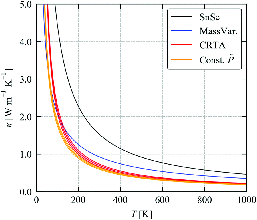 | ||
| Fig. 10 Predicted averaged thermal conductivity κave of SnSe (black) and the κave of Sn(S0.1875Se0.8125) obtained using the three models considered in this section: the mass-variance model (blue), the CRTA model defined in eqn (3) and (4) with an interpolated lifetime τCRTA (red), and the model defined in eqn (8) with the interaction strengths Pλ replaced by an interpolated constant (orange). | ||
Within the CRTA model, the majority of the reduction in the κlatt is due to a reduced harmonic term which, to the extent that thermodynamic model for the alloy is reasonable, is not approximated in this work. The small difference between the CRTA and constant then points to a small potential secondary effect from changes in the phonon lifetimes due to changes in the phonon frequency spectrum. While we cannot rule out changes in the phonon–phonon interaction strengths in the alloy, for a near-ideal solid solution like Sn(S1−xSex) it seems reasonable to assume that the averaged can be interpolated. The performance of the simple mass-variance model is remarkable given that it is much less computationally demanding than either of the other two approaches, and suggests it may be a good initial approach to predicting the κlatt of alloy systems.
Finally, we should also note that the virtual crystal approximation (VCA) might be a useful “middle ground” between the simple mass-variance model and the more sophisticated CRTA and constant interaction-strength models. In the VCA, the force constants for an alloy are built from appropriate linear combinations of the force constants of the endpoints, which in principle improves on the average mass model by accounting for changes in the second- and third-order force constants.32 Unfortunately, this technique is presently not implemented in the Phono3py software, so we were not able to test it alongside the other methods.
4. Conclusions
In summary, we have performed a detailed characterisation of the thermal conductivity of SnS and SnSe and of the Sn(S0.1875Se0.8125) alloy.In these calculations, we find that SnS and SnSe have similar, ultra-low κlatt, and the difference between them is down to a subtle balance of decreased group velocities but longer lifetimes in the selenide. The longer lifetimes are due to weaker phonon–phonon interaction strengths, and negate an increase in the number of energy- and momentum-conserving scattering pathways due to the smaller range of phonon frequencies.
Our thermodynamic model of Sn(S0.1875Se0.8125) indicates near-ideal behaviour, with the mixing free energy dominated by entropy and a close-to homogenous distribution of occurrence probabilities over the 23 independent chalcogen arrangements in our 32-atom alloy supercell. In contrast to our previous work, we find that vibrational contributions to the free energy have a relatively small impact on the thermodynamics. While this result may be taken as an indication that vibrational effects need not be taken into account in alloy models, further work is required to determine whether this generalises to less ideal solid solutions.
By performing harmonic phonon calculations on the alloy model, we investigated three possible approaches to quantifying the impact of alloying on the thermal transport and predicted a substantial 40–60% drop in the κlatt compared to the SnSe endpoint. Our analysis suggests the majority of this is due to a reduction in the group velocities, which also manifests as a “smearing” of the phonon dispersion, together with a small additional effect from a reduction in the phonon lifetimes. We also found that a simple isotope-scattering model provided a good reproduction of the results obtained using more sophisticated – and more computationally-demanding – models, and it is therefore of interest to investigate whether this is more generally applicable.
Overall, this study has provided useful insight into how alloying reduces the thermal conductivity of SnS and SnSe, and we hope these theoretical models will be of use to modelling studies on other widely-used thermoelectrics in the future. Ultimately, we hope that microscopic insight from first-principles calculations such as these will be able to inform the future selection of alloy systems to optimise the thermoelectric performance of existing and novel TEs. With regard to the SnS/SnSe system, the preservation of the structure in the low-frequency dispersion of Sn(S0.1875Se0.8125), together with the large impact of changes in group velocity in reducing the κlatt, suggests that it may be of interest to consider (Ge1−xSnx)S or (Ge1−xSnx)Se alloys as alternatives.
Data-access statement
Raw data from our previous studies on the Snn(S1−xSex)m and Pnma Sn(S1−xSex) solid solutions is available free of charge in online repositories (ref. 40 and 61). Raw data from this study is also available free of charge online at: http://dx.doi.org/10.17632/hrzkm56zw7.1. A set of utilities and analysis codes for Phonopy and Phono3py calculations are available in a GitHub repository: https://github.com/skelton-group/Phono3py-Power-Tools. Any data not included in the data repositories is available from the authors on reasonable request.Conflicts of interest
There are no conflicts to declare.Acknowledgements
JS is grateful to UK Research and Innovation for the award of a Future Leaders Fellowship (grant no. MR/T043121/1), and he previously held a Presidential Fellowship at the University of Manchester. The majority of the calculations reported in this work made use of the UK Archer and Archer 2 facilities, via JS's membership of the UK Materials Chemistry Consortium, which is funded by the UK Engineering and Physical Sciences Research Council (grant no. EP/L000202, EP/R029431 and EP/T022213). Calculations were also performed using the UoM Computational Shared Facility, which is maintained by UoM Research IT.References
- R. Freer and A. V. Powell, J. Mater. Chem. C, 2020, 8, 441–463 Search PubMed.
- G. Tan, L.-D. Zhao and M. G. Kanatzidis, Chem. Rev., 2016, 116, 12123–12149 Search PubMed.
- G. L. Bennett, J. J. Lombardo, R. J. Hemler, G. Silverman, C. W. Whitmore, W. R. Amos, E. W. Johnson, R. W. Zocher, J. C. Hagan and R. W. Englehart, AIP Conference Proceedings, AIP, 2008, vol. 969, pp. 663–671 Search PubMed.
- J. M. Dilhac, R. Monthéard, M. Bafleur, V. Boitier, P. Durand-Estèbe and P. Tounsi, J. Electron. Mater., 2014, 43, 2444–2451 Search PubMed.
- Q. Huang, C. Lu, M. Shaurette and R. F. Cox, in Proceedings of the 28th International Symposium on Automation and Robotics in Construction, ISARC 2011, International Association for Automation and Robotics in Construction (I.A.A.R.C), 2011, pp. 1376–1380 Search PubMed.
- J. J. Kuchle and N. D. Love, Meas. J. Int. Meas. Confed., 2014, 47, 26–32 Search PubMed.
- J. Yang and F. R. Stabler, in Journal of Electronic Materials, Springer, 2009, vol. 38, pp. 1245–1251 Search PubMed.
- Z. Yang, J. Pradogonjal, M. Phillips, S. Lan, A. Powell, P. Vaqueiro, M. Gao, R. Stobart and R. Chen, in SAE Technical Papers, SAE International, 2017, vol. 2017 – March Search PubMed.
- Y.-M. Han, J. Zhao, M. Zhou, X.-X. Jiang, H.-Q. Leng and L.-F. Li, J. Mater. Chem. A, 2015, 3, 4555–4559 Search PubMed.
- Asfandiyar, T.-R. Wei, Z. Li, F.-H. Sun, Y. Pan, C.-F. Wu, M. U. Farooq, H. Tang, F. Li, B. Li and J.-F. Li, Sci. Rep., 2017, 7, 43262 Search PubMed.
- C.-C. Lin, R. Lydia, J. H. Yun, H. S. Lee and J. S. Rhyee, Chem. Mater., 2017, 29, 5344–5352 Search PubMed.
- H. Xie, X. Su, S. Hao, C. Zhang, Z. Zhang, W. Liu, Y. Yan, C. Wolverton, X. Tang and M. G. Kanatzidis, J. Am. Chem. Soc., 2019, 141, 18900–18909 Search PubMed.
- K. Biswas, J. He, I. D. Blum, C.-I. Wu, T. P. Hogan, D. N. Seidman, V. P. Dravid and M. G. Kanatzidis, Nature, 2012, 489, 414–418 Search PubMed.
- J. R. Sootsman, D. Y. Chung and M. G. Kanatzidis, Angew. Chem., Int. Ed., 2009, 48, 8616–8639 Search PubMed.
- S. Hébert, D. Berthebaud, R. Daou, Y. Bréard, D. Pelloquin, E. Guilmeau, F. Gascoin, O. Lebedev and A. Maignan, J. Phys.: Condens. Matter, 2016, 28, 013001 Search PubMed.
- J. W. G. Bos and R. A. Downie, J. Phys.: Condens. Matter, 2014, 26, 433201 Search PubMed.
- J. Shuai, J. Mao, S. Song, Q. Zhang, G. Chen and Z. Ren, Mater. Today Phys., 2017, 1, 74–95 Search PubMed.
- J. A. Dolyniuk, B. Owens-Baird, J. Wang, J. V. Zaikina and K. Kovnir, Mater. Sci. Eng., R, 2016, 108, 1–46 Search PubMed.
- M. Rull-Bravo, A. Moure, J. F. Fernández and M. Martín-González, RSC Adv., 2015, 5, 41653–41667 Search PubMed.
- L.-D. Zhao, S.-H. Lo, Y. Zhang, H. Sun, G. Tan, C. Uher, C. Wolverton, V. P. Dravid and M. G. Kanatzidis, Nature, 2014, 508, 373–377 Search PubMed.
- L.-D. Zhao, G. Tan, S. Hao, J. He, Y. Pei, H. Chi, H. Wang, S. Gong, H. Xu, V. P. Dravid, C. Uher, G. J. Snyder, C. Wolverton and M. G. Kanatzidis, Science, 2016, 351, 141–144 Search PubMed.
- C. W. Li, J. Hong, A. F. May, D. Bansal, S. Chi, T. Hong, G. Ehlers and O. Delaire, Nat. Phys., 2015, 11, 1063–1069 Search PubMed.
- J. M. Skelton, L. A. Burton, S. C. Parker, A. Walsh, C.-E. Kim, A. Soon, J. Buckeridge, A. A. Sokol, C. R. A. Catlow, A. Togo and I. Tanaka, Phys. Rev. Lett., 2016, 117, 075502 Search PubMed.
- U. Aseginolaza, R. Bianco, L. Monacelli, L. Paulatto, M. Calandra, F. Mauri, A. Bergara and I. Errea, Phys. Rev. Lett., 2019, 122, 075901 Search PubMed.
- J. M. Skelton, L. A. Burton, A. J. Jackson, F. Oba, S. C. Parker and A. Walsh, Phys. Chem. Chem. Phys., 2017, 19, 12452–12465 Search PubMed.
- U. Aseginolaza, R. Bianco, L. Monacelli, L. Paulatto, M. Calandra, F. Mauri, A. Bergara and I. Errea, Phys. Rev. B, 2019, 100, 214307 Search PubMed.
- Q. Tan, L.-D. Zhao, J.-F. Li, C.-F. Wu, T.-R. Wei, Z.-B. Xing and M. G. Kanatzidis, J. Mater. Chem. A, 2014, 2, 17302–17306 Search PubMed.
- B. Zhou, S. Li, W. Li, J. Li, X. Zhang, S. Lin, Z. Chen and Y. Pei, ACS Appl. Mater. Interfaces, 2017, 9, 34033–34041 Search PubMed.
- A. Togo and I. Tanaka, Scr. Mater., 2015, 108, 1–5 Search PubMed.
- W. Li, J. Carrete, N. A. Katcho and N. Mingo, Comput. Phys. Commun., 2014, 185, 1747–1758 Search PubMed.
- A. Togo, L. Chaput and I. Tanaka, Phys. Rev. B: Condens. Matter Mater. Phys., 2015, 91, 094306 Search PubMed.
- J. Carrete, B. Vermeersch, A. Katre, A. van Roekeghem, T. Wang, G. K. H. Madsen and N. Mingo, Comput. Phys. Commun., 2017, 220, 351–362 Search PubMed.
- W. Rahim, J. M. Skelton and D. O. Scanlon, J. Mater. Chem. A, 2020, 8, 16405–16420 Search PubMed.
- J. Tang and J. M. Skelton, J. Phys.: Condens. Matter, 2021, 33, 164002 Search PubMed.
- J. Carrete, W. Li, N. Mingo, S. Wang and S. Curtarolo, Phys. Rev. X, 2014, 4, 011019 Search PubMed.
- P. Gorai, E. S. Toberer and V. Stevanović, J. Mater. Chem. A, 2016, 4, 11110–11116 Search PubMed.
- R. Li, X. Li, L. Xi, J. Yang, D. J. Singh and W. Zhang, ACS Appl. Mater. Interfaces, 2019, 11, 24859–24866 Search PubMed.
- D. S. D. Gunn, J. M. Skelton, L. A. Burton, S. Metz and S. C. Parker, Chem. Mater., 2019, 31, 3672–3685 Search PubMed.
- J. M. Skelton and J. Phys, Energy, 2020, 2, 025006 Search PubMed.
- J. Skelton, D. Gunn, L. Burton, S. Metz and S. Parker, Mendeley Data, Version 3, , 2020 DOI:10.17632/BWHJG65XVD.3.
- G. Kresse and J. Hafner, Phys. Rev. B: Condens. Matter Mater. Phys., 1993, 47, 558(R)–561(R) Search PubMed.
- J. P. Perdew, A. Ruzsinszky, G. I. Csonka, O. A. Vydrov, G. E. Scuseria, L. A. Constantin, X. Zhou and K. Burke, Phys. Rev. Lett., 2008, 100, 136406 Search PubMed.
- S. Grimme, J. Antony, S. Ehrlich and H. Krieg, J. Chem. Phys., 2010, 132, 154104 Search PubMed.
- H. J. Monkhorst and J. D. Pack, Phys. Rev. B: Solid State, 1976, 13, 5188–5192 Search PubMed.
- P. E. Blöchl, Phys. Rev. B: Condens. Matter Mater. Phys., 1994, 50, 17953–17979 Search PubMed.
- G. Kresse and D. Joubert, Phys. Rev. B: Condens. Matter Mater. Phys., 1999, 59, 1758–1775 Search PubMed.
- P. B. Allen, T. Berlijn, D. A. Casavant and J. M. Soler, Phys. Rev. B: Condens. Matter Mater. Phys., 2013, 87, 085322 Search PubMed.
- J. M. Skelton, L. A. Burton, F. Oba and A. Walsh, J. Phys. Chem. C, 2017, 121, 6446–6454 Search PubMed.
- I. Pallikara and J. Skelton, ChemRxiv Preprint, 2021 DOI:10.26434/CHEMRXIV.14187689.V1.
- K. Momma and F. Izumi, J. Appl. Crystallogr., 2011, 44, 1272–1276 Search PubMed.
- T. Chattopadhyay, J. Pannetier and H. G. von Schnering, J. Phys. Chem. Solids, 1986, 47, 879–885 Search PubMed.
- J. M. Skelton, L. A. Burton, A. J. Jackson, F. Oba, S. C. Parker and A. Walsh, Phys. Chem. Chem. Phys., 2017, 19, 12452 Search PubMed.
- P. C. Wei, S. Bhattacharya, J. He, S. Neeleshwar, R. Podila, Y. Y. Chen and A. M. Rao, Nature, 2016, 539, E1–E2 Search PubMed.
- L. D. Zhao, S. H. Lo, Y. Zhang, H. Sun, G. Tan, C. Uher, C. Wolverton, V. P. Dravid and M. G. Kanatzidis, Nature, 2016, 539, E2–E3 Search PubMed.
- Y. Li, B. He, J. P. Heremans and J. C. Zhao, J. Alloys Compd., 2016, 669, 224–231 Search PubMed.
- T. Feng, A. O’Hara and S. T. Pantelides, Nano Energy, 2020, 75, 104916 Search PubMed.
- G. K. H. Madsen and D. J. Singh, Comput. Phys. Commun., 2006, 175, 67–71 Search PubMed.
- R. Grau-Crespo, S. Hamad, C. R. A. Catlow and N. H. de Leeuw, J. Phys.: Condens. Matter, 2007, 19, 256201 Search PubMed.
- S. I. Tamura, Phys. Rev. B: Condens. Matter Mater. Phys., 1983, 27, 858–866 Search PubMed.
- H. Yang, C. N. Savory, B. J. Morgan, D. O. Scanlon, J. M. Skelton and A. Walsh, Chem. Mater., 2020, 32, 7542–7550 Search PubMed.
- J. Skelton, Mendeley Data, Version 1, , 2020 DOI:10.17632/M34BNMPKPX.1.
Footnote |
| † Electronic supplementary information (ESI) available. See DOI: 10.1039/d1tc02026a |
| This journal is © The Royal Society of Chemistry 2021 |