 Open Access Article
Glassy dynamics of sticky hard spheres beyond the mode-coupling regime
Chengjie
Luo
 and
Liesbeth M. C.
Janssen
 *
*
Department of Applied Physics, Eindhoven University of Technology, Eindhoven, The Netherlands. E-mail: l.m.c.janssen@tue.nl
First published on 4th August 2021
Abstract
Sticky hard spheres, i.e., hard particles decorated with a short-ranged attractive interaction potential, constitute a relatively simple model with highly non-trivial glassy dynamics. The mode-coupling theory of the glass transition (MCT) offers a qualitative account of the complex reentrant dynamics of sticky hard spheres, but the predicted glass transition point is notoriously underestimated. Here we apply an improved first-principles-based theory, referred to as generalized mode-coupling theory (GMCT), to sticky hard spheres. This theoretical framework seeks to go beyond MCT by hierarchically expanding the dynamics in higher-order density correlation functions. We predict the phase diagrams from the first few levels of the GMCT hierarchy and the dynamics-related critical exponents, all of which are much closer to the empirical observations than MCT. Notably, the prominent reentrant glassy dynamics, the glass–glass transition, and the higher-order bifurcation singularity classes (A3 and A4) of sticky hard spheres are found to be preserved within GMCT at arbitrary order. Moreover, we demonstrate that when the hierarchical order of GMCT increases, the effect of the short-ranged attractive interactions becomes more evident in the dynamics. This implies that GMCT is more sensitive to subtle microstructural differences than MCT, and that the framework provides a promising first-principles approach to systematically go beyond the MCT regime.
1 Introduction
The dynamics of supercooled liquids and the nature of the glass transition are still not fully understood from a theoretical perspective.1,2 It is empirically well established that supercooling of a liquid is accompanied by a spectacular slowdown in dynamics over many orders of magnitude; at the same time, however, the disordered microstructure of the material remains very close to that of a normal liquid.3 One of the major challenges is to explain this emergent slow relaxation dynamics of glass-forming liquids on the basis of the material's static structure. At present, there are many theories that seek to answer this question, ranging from e.g. geometric-frustration-based theories4 to spin-glass-inspired approaches such as Random First Order Transition theory.5 More recently, machine learning has also been used to search for the link between structure and dynamics in dense disordered systems.6–9 However, there is still no complete and formally exact theory of glassy dynamics that is founded entirely on first principles.Mode-coupling theory (MCT), developed in the 1980s by Götze and co-workers,3,10–13 is an approximate framework that is widely regarded as the only first-principles-based theory of the glass transition. For a review of this theory we refer the reader to ref. 3, 12 and 13. Briefly, among the main successes of MCT is its qualitative prediction of the non-trivial dynamical slowdown – as characterized by the intermediate scattering function F(k, t) for a given wavenumber k and time t – based on only small changes in the static structure factor S(k). For supercooled liquids, MCT typically predicts a two-step decay of F(k, t) via the so-called β- and α-relaxation processes, respectively, with a long plateau emerging at intermediate time scales. This plateau, which becomes longer upon deeper supercooling, is indicative of solid-like behavior and can also be understood in terms of the cage effect. Moreover, MCT predicts several scaling laws for the intermediate scattering function in the β- and α-relaxation regimes that are generally consistent with the behavior seen in experimental glass-forming systems. When the temperature further decreases to a certain value, MCT predicts a liquid–glass transition at which the long-time limit of the intermediate scattering function, also called the non-ergodicity parameter, jumps discontinuously from zero to a positive value. Many of the non-ergodicity parameters of different glass-forming materials are accurately predicted from MCT.3,14 However, owing to its approximate nature, MCT is also known to become inaccurate or can even break down in certain cases. The main MCT approximation stems from the fact that the intermediate scattering function F(k, t), which in fact is a two-point density correlation function, is determined by a memory function in which four-point density correlation functions are required as the leading terms. In standard MCT, these four-point density correlation functions are approximated by the product of two F(k, t) functions at different wavenumbers.3 This approximation is generally not accurate enough and is even uncontrolled.13 Additionally, the four-point density correlation functions may contain information on non-trivial spatiotemporal density fluctuations related to dynamical heterogeneity, but these non-trivial correlations are inherently lost when applying the MCT factorization approximation.15–18 Hence, a more accurate theory taking multi-point density correlators into account is needed.
Recently, a new theory called generalized mode-coupling theory (GMCT) has been developed based on the framework of MCT.19–21 Within this theory, the uncontrolled approximation for the four-point density correlation functions is avoided by developing an exact dynamical equation for the four-point density correlators themselves; these are governed by a new memory function that is dominated by six-point density correlations, which in turn are controlled by eight-point correlators, et cetera. One may then apply a generalized MCT closure approximation at an arbitrary level in this hierarchy, thus delaying the uncontrolled factorization to a later stage. In this way, more accurate predictions for the relaxation dynamics can be obtained by systematically including higher-level correlation functions, which in fact establishes a hierarchy of coupled integro-differential equations. We note that, similar to MCT, the only material-dependent input for the theory is still the static structure factor S(k) for any given temperature and density.
GMCT has been well studied for hard-sphere systems with a hard-core repulsive interaction potential.21–23 It has been found that GMCT indeed systematically improves the predictions from MCT. More specifically, the location of the liquid–glass transition point, which is usually underestimated in MCT, improves in a seemingly convergent manner as higher-order density correlations are included in the first few levels of the GMCT hierarchy.19–22 Moreover, the qualitative MCT scaling laws near the liquid–glass transition in the β- and α-relaxation regimes are fully preserved in GMCT, but with quantitatively systematically improved exponents.22,23 These triumphs of GMCT make it a promising first-principles-based theory for the glass transition, although it must be noted that the computational cost of a numerical GMCT calculation heavily increases with the number of included hierarchical levels, both in terms of computing time and required computer memory.22
Despite the promising GMCT results for hard spheres, many real glass-forming materials are governed by more complex interaction potentials between the particles. Standard MCT has already been widely tested for different glass-forming materials, including model systems interacting through Lennard-Jones potentials,24,25 amorphous metal alloys,26,27 colloidal suspensions,28–30 polymers,31,32 vitrimers,33 and systems interacting through many-body potentials.34 In all of these systems, MCT qualitatively captures at least some key features of the glassy dynamics. A natural question is whether GMCT is also applicable for these more complex glass formers. To address this question, we will take the so-called sticky hard sphere model, which is characterized by a hard-core repulsive potential with a short-ranged attractive square well, as our system of study.
The sticky hard sphere model is the simplest model with both repulsive and attractive interactions but with rich dynamical behavior. In the last 20 years, many simulation35–46 and experimental47–56 studies have been performed for this model. It is widely accepted that there exists a complex reentrant dynamics when decreasing the temperature of the system at certain fixed values of the packing fraction and potential well width. Moreover, in contrast to the typical power-law decays of the intermediate scattering function near the critical liquid–glass point for hard spheres, an anomalous logarithmic decay has been found for sticky hard spheres. Although still debated recently,57 the sticky hard-sphere reentrance is associated with two distinct types of glass: one is the so-called attractive glass, or bonded glass, related to the short deep potential well; the other is the repulsive glass, or non-bonded glass, similar to the hard-sphere glass. In MCT, all the above properties have been successfully predicted. Moreover, MCT predicts a glass–glass transition and even more complex transitions called A3 and A4 singularities, which can also explain the logarithmic decay of the intermediate scattering function.58 However, we point out that the predictions from MCT are all qualitatively but not quantitatively correct. For example, regarding the phase transition at different well widths, the critical packing fractions are all underestimated by MCT. Furthermore, the A3 and A4 singularity points predicted by MCT have to be rescaled to match the simulation or experimental results.39,49 In this work, we revisit the sticky hard sphere model in the context of GMCT, with the aim to test the applicability of GMCT for systems with both attractive and repulsive interactions, and to establish to what extent first-principles predictions for glassy sticky hard spheres can be improved.
The outline of this paper is as follows. We first introduce the microscopic GMCT framework and the related analytical scaling laws. We also briefly describe the sticky hard sphere model and the numerical details for the application of GMCT to this model. Subsequently, we present the rich phase diagrams of sticky hard spheres predicted from higher-order GMCT and compare them to literature to demonstrate the quantitative improvement attained by GMCT. Next, we discuss the non-ergodicity parameters at the critical points for both the liquid–glass transitions and the glass–glass transition, reflecting the different mechanisms of the two types of glass. The exponent parameters that characterize the dynamics near the corresponding critical points are also provided. Finally, we show the relaxation dynamics near the higher-order A3 and A4 singularities, demonstrating that the pronounced logarithmic decay of the dynamical density correlation functions is preserved within higher-order GMCT. We conclude with some critical remarks and perspectives for future work.
2 Theory
2.1 Generalized mode-coupling theory
We first review the microscopic GMCT equations of motion21 and several scaling laws derived from them.23 The microscopic dynamical information of a glass-forming material is assumed to be encoded in the 2n-point density correlation functions Fn(k1,…,kn, t), defined as| Fn(k1,…,kn, t) = 〈ρ−k1(0)…ρ−kn(0)ρk1(t)…ρkn(t)〉, | (1) |
 is a collective density mode at wavevector k and time t, Np is the total number of particles, the angle brackets denote an ensemble average, and the label n (n = 1,…,∞) specifies the level of the GMCT hierarchy. Note that when n = 1, F1(k, t) is the intermediate scattering function. In the overdamped limit, the GMCT equations read
 | (2) |
 | (3) |
 | (4) |
 | (5) |
| Vq,k−q = (k·q)c(q) + k·(k − q)c(|k − q|), | (6) |
In principle, one should expand the GMCT equations up to n → ∞ to obtain the correct dynamical density correlations. However, in practice we can only solve the GMCT equations up to a finite level N < ∞, which necessitates the use of a closure approximation for the last included level N. There are two kinds of GMCT closures that have been well-studied before.21,22 One kind is the so-called mean-field (MF) closure, which approximates the highest-order correlator FN as a product of lower-order dynamical density correlation functions. In this paper, we only focus on one such example, for N > 2,
 | (7) |
Eqn (2), (5), and (7) define a unique time-dependent solution Fn(k1,…,kn, t) for n ≤ N.63 Before we go to the specific model and the numerical calculation, let us discuss some universal properties of the GMCT solutions which can be obtained from mathematically analyzing the equations.
Firstly, using the Laplace transform and the final value theorem, the long-time limit of the multi-point density correlation function  can be calculated via
| Fn(k1,…,kn) = Sn(k1,…,kn) − [Sn−1(k1,…,kn) + Jn−2(k1,…,kn)Mn(k1,…,kn)]−1, | (8) |
 represents the long-time limit of the memory function. When n < N,
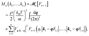 | (9) |
 | (10) |
![[scr M, script letter M]](https://www.rsc.org/images/entities/char_e145.gif) to denote the memory functionals. The solutions of eqn (8)–(10) can exhibit non-trivial singularities that may be analyzed using the Jacobian of these equations. The Jacobian is equivalent to 1 − C, where C is the stability matrix of eqn (8)–(10) which satisfies
to denote the memory functionals. The solutions of eqn (8)–(10) can exhibit non-trivial singularities that may be analyzed using the Jacobian of these equations. The Jacobian is equivalent to 1 − C, where C is the stability matrix of eqn (8)–(10) which satisfies| H = CH. |
| Here H is a vector in the form of [{H1(k1)}∀k1, {H2(k1, k2)}∀k1,∀k2,…,{Hn(k1,…,kn)}∀k1,…,∀kn]T. Explicitly, for n < N, |
Hn(k1,…,kn) = [Sn(k1,…,kn) − Fn(k1,…,kn)]2Jn−2(k1,…,kn) × ![[scr M, script letter M]](https://www.rsc.org/images/entities/char_e145.gif) n[Hn+1]. n[Hn+1]. | (11) |
HN(k1,…,kN) = [SN(k1,…,kN) − FN(k1,…,kN)]2JN−2(k1,…,kN) × {![[scr M, script letter M]](https://www.rsc.org/images/entities/char_e145.gif) N[MN−1,H1] + N[MN−1,H1] + ![[scr M, script letter M]](https://www.rsc.org/images/entities/char_e145.gif) N[ N[![[scr M, script letter M]](https://www.rsc.org/images/entities/char_e145.gif) N−1[HN], F1]}. N−1[HN], F1]}. | (12) |
At each singularity point, i.e., when E = 1, the left eigenvector ên(k1,…,kn) and right eigenvector en(k1,…,kn) of the C matrix can be obtained with conventions
 | (13) |
 represents the summation over all possible wavenumbers k1,…,km for level m and the superscript c refers to the critical-point values. The above eigenvectors are used to characterize every transition point by a single number λ, defined as
 | (14) |
Let us briefly summarize some leading order scaling laws near A2 singularities within the framework of GMCT, both for the normalized long-time limits of the density correlators and for the time-dependent ones [i.e., the solutions of eqn (2), (5) and (7)]. Details of these scaling laws can be found in ref. 23. Here the control parameter is the relative distance to a A2 critical point which, for example, is measured by the packing fraction in hard spheres, ε = (φ − φc)/φc.
• If ε > 0 and |ε| ≪ 1, the system is in the glass state and the non-ergodicity parameters scale with  as
as
 | (15) |
| hn(k1,…,kn) = en(k1,…,kn)/Sn(k1,…,kn). | (16) |
• If |ε| ≪ 1, the β-relaxation regime can be characterized by a unique timescale τβ ∼ |ε|−1/2a. In this regime, the dynamical normalized density correlation functions fn(k1,…,kn, t) ≡ Fn(k1,…,kn, t)/Sn(k1,…,kn) obey a time-wavenumber factorization property such that
| fn(k1,…,kn, t) = fcn(k1,…,kn, t) + hn(k1,…,kn, t)G(t). | (17) |
 , with the subscript ± denoting the sign of ε. For the limiting case that ε → 0−, i.e., on the liquid side of the transition, the β-correlator satisfies
 | (18) |
 | (19) |
| λ = Γ(1 − a)2/Γ(1 − 2a) = Γ(1 + b)2/Γ(1 + 2b). | (20) |
| γ = 1/2a + 1/2b. | (21) |
• If ε < 0 and |ε| ≪ 1, the system is in the liquid state and the dynamical normalized density correlation functions in the α-relaxation regime obey a time-density superposition principle
fn(k1,…,kn, t) = ![[f with combining tilde]](https://www.rsc.org/images/entities/i_char_0066_0303.gif) n(k1,…,kn, t/τ). n(k1,…,kn, t/τ). | (22) |
For higher-order singularities Al with l > 2, a major difference with the scaling laws above is that near such singularities, to leading order in  , the β-correlators G(t) may follow a logarithmic decay,58,66i.e.
 | (23) |
σ|ε| − s2G2(s) + s![[script L]](https://www.rsc.org/images/entities/char_e144.gif) [G2(t)] = 0 [G2(t)] = 0 | (24) |
2.2 Sticky hard sphere model
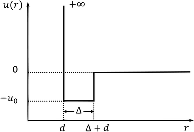
We apply our GMCT framework to a system composed of sticky hard spheres. The pair interaction potential of this system includes both a repulsive and attractive part, as shown in Fig. 1. Within the particle diameter d, the value of the potential is u(r) = +∞, which accounts for hard-core repulsion to prevent particle overlap. Outside the hard-core region there is a small square potential well with width Δ ≪ d, i.e., for d < r < d + Δ we have u(r) = −u0, with u0 > 0. Thus, if the distance of two particles falls within this range, the particles will attract each other to be sticky. When r > d + Δ, u(r) = 0.There are three independent parameters of this model. One is the packing fraction φ = πρd3/6. The second is the reduced temperature θ, defined as the inverse of the attraction well depth over thermal energy, i.e., θ = kBT/u0. The third one is the relative width of the well, δ = Δ/d. Note that when u0 = 0 (θ → ∞), this sticky hard sphere model reduces to the hard sphere model and the only parameter is the packing fraction φ. We calculate the structure factors S(k) from the pair potential using the Ornstein–Zernike equation together with the mean-spherical approximation.59 More specifically, we use the approach motivated by Baxter's theory in ref. 58 to numerically obtain the structure factors in the three-dimension control parameter space (φ, θ, δ); these structure factors subsequently serve as our GMCT input.
For the GMCT calculations, we numerically solve eqn (2)–(7) for the time-dependent dynamics of the multi-point density correlation functions, and eqn (8)–(10) for the corresponding long-time limits, for MF closure levels N = 2, 3, 4. The wavevector-dependent integrals over q in the memory functions are approximated as a double Riemann sum68 with an equidistant wavenumber grid of Nk = 500 points that ranges from kd = 0.2 to kd = 200.2. Such a fine wavenumber grid is necessary to reach convergence, in particular for low values of θ. For the time-dependent solutions we use the integration algorithm described by Fuchs et al.,69 starting with a time step size of Δt = 10−6 that is subsequently doubled every 32 points. In all our GMCT calculations we set kB/m = 1 and the effective friction coefficients νn = 1 for 1 ≤ n ≤ N.
3 Results and discussion
3.1 Phase diagram
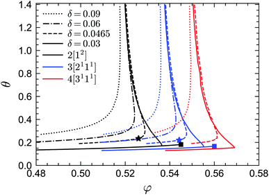
We first report the GMCT phase diagrams in the (φ, θ) plane for several fixed values of δ (i.e., fixed potential well widths), as shown in Fig. 2. Let us start by discussing the N = 2 results, which are also fully consistent with the standard-MCT results of approximately 20 years ago.58 For all values of δ considered (δ = 0.09, 0.06, 0.0465, 0.03), a common phenomenon is that for a given reduced temperature θ, there is always a liquid–glass transition point φc. That is, for φ > φc the non-ergodicity parameters are larger than zero and the system is in the glass state, while for φ < φc the non-ergodicity parameters are all 0, representing a liquid state. Thus, for an arbitrary temperature and potential well width, one may always find an ergodicity-breaking transition by going to sufficiently high packing fractions. However, for a given packing fraction, the influence of the reduced temperature is more subtle and depends on the width of the potential well. At relatively large widths, such as δ = 0.09, the picture is fairly trivial: the lower the temperature, the more glassy the system. This is indeed similar to systems with a relatively large attractive potential well, such as the Lennard-Jones potential.24 Conversely, when the width of the attractive well decreases to e.g. δ = 0.06, the scenario changes: at high temperatures the system is in the glass state, at lower temperatures the glass melts into a liquid state, and finally at even lower temperatures the system re-enters the glass phase. This is the famous reentrant phenomenon of systems with a short attractive well, and can be found regardless of the shape of the well.70 Physically, the existence of the glass phase at high reduced temperatures (i.e., the repulsive glass) can be understood in terms of the cage effect, similar to the case of hard spheres. That is, the MCT modes with wavelengths close to the average distance of neighbors play the dominant role. By contrast, the glass phase at low temperatures (i.e., the so-called attractive glass) arises from particle bonding, with the MCT modes at wavelengths comparable to the width of the attractive potential well becoming more important. The liquid state in between can be explained by the following two arguments:49,58 (i) compared to the repulsive glass, the attraction causes the separation of two particles to be smaller so that the average size of the free space increases, facilitating longer-distance particle motion and thus faster structural relaxation; (ii) compared to the attractive glass, the “stickiness” between particles is weaker, hence the particles have a higher probability to break their bonds and move relatively fast away from their initial positions.The two-glass picture becomes a glass–glass transition for very small potential well widths. For example, when δ = 0.03, in addition to the reentrant liquid–glass transition, there is another A2 glass–glass transition predicted from MCT (black solid line from the crossing point near φ = 0.535 to the black square marker in Fig. 2). The existence of this glass–glass transition is still debated, most recently based on swap Monte Carlo simulations,57 but from the theoretical point of view, this transition indeed exists since the maximum eigenvalue E of the C matrix introduced in the previous section is unity at the glass–glass transition curve, with λ < 1. Moreover, when δ = 0.03, along the A2 glass–glass transition curve, λ increases with increasing φ until λ → 1 (black solid line in Fig. 9) indicating an end point with an A3 singularity (black square in Fig. 2). When increasing the width δ, the length of the glass–glass transition curve shrinks and there will be a δ* at some φ* and θ* when the curve vanishes. The point (φ*, θ*, δ*) is the A4 singularity (black star in Fig. 2).
While standard MCT already successfully captures the two competing effects, i.e., caging and bonding, underlying vitrification in sticky hard spheres, the MCT-predicted phase diagram is not quantitative accurate. Indeed, as in many other systems, MCT generally tends to overestimate the critical packing fraction of the liquid–glass transition point. Let us therefore turn to the higher-order GMCT results in Fig. 2. We find that overall the shape of the phase diagram under higher-order MF closures remains similar to the MCT case, with all the liquid–glass transitions, glass–glass transitions and Al (l = 2, 3, 4) singularities preserved. However, when the MF closure level N in GMCT increases, all the phase transition curves for a given δ move to larger packing fraction values. Note also that at high reduced temperatures θ, the critical liquid–glass transition points at different widths δ will converge to the corresponding GMCT critical points for hard spheres. It has been shown that the GMCT-predicted critical packing fraction φc for hard spheres shifts toward higher values in a seemingly convergent manner, i.e., the difference φc(N) − φc(N − 1) becomes increasingly smaller as N increases.22 The phase transition curves in Fig. 2 also imply this uniform convergence for any given δ and θ. This is arguably one of the biggest triumphs of GMCT: by systematically including higher levels of density correlators in the GMCT hierarchy, the critical point can be systematically improved, even in the presence of competing repulsive and attractive particle interactions.
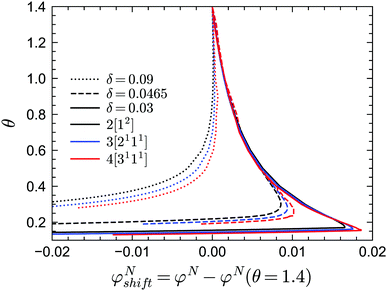
In practice, the phase transition lines from MCT are usually shifted or rescaled to compare with simulation or experimental results. In Fig. 3 we present the shifted GMCT liquid–glass transition curves for N = 2, 3, 4 relative to the corresponding critical points φN(θ = 1.4) at each δ. We have chosen θ = 1.4, which is approximately equivalent to the hard-sphere limit, as a reference point for convenience. For each δ value, it is obvious that the shifted phase transition curves at different closure levels N do not collapse to a single curve, especially at low temperatures θ. This indicates that the GMCT-predicted phase diagrams under higher closure levels are non-trivial in the sense that they cannot be obtained by simply shifting the MCT results. At high δ, such as δ = 0.09, increasing N leads to larger shifted critical packing fractions φNshift of the liquid–glass transition (dotted lines in Fig. 3). Moreover, the difference between the φNshift with N = 3 (or N = 4) and the one with N = 2, i.e., ΔφN=3shift ≡ φN=3shift − φN=2shift, is larger at low θ. This implies that the higher order density correlations included in GMCT may contribute more to the dynamics when the attractive potential well is deeper. However, when δ decreases to e.g. δ = 0.03 (solid lines in Fig. 3 and 4), the relation between the temperature θ and the shifted liquid–glass transition lines becomes more complex. At low temperatures, when N increases, the shifted critical packing fractions φNshift increase as well, which is similar to the δ = 0.09 case. However, at higher temperatures, φNshift decreases as the level N increases. There thus exists a crossing point between any two shifted phase transition curves with different closure levels N; this crossing point (θ ≈ 0.22, φNshift ≈ 0.015) is close to the ‘convex’ part of the phase diagram, and more specifically at the high-temperature side of the convex region. The ΔφNshift shown in the inset of Fig. 4 demonstrates this opposite trend for relatively high and low temperatures.
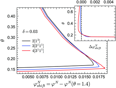 | ||
| Fig. 4 Shifted liquid–glass transition lines of sticky hard spheres for different GMCT MF closure levels at a relative attraction well width of δ = 0.03. The results are the same as in Fig. 3 but enlarged for the low reduced-temperature region. The inset shows the difference between the higher-order GMCT and MCT curves of the main panel, i.e. ΔφNshift ≡ φNshift − φNshift= 2. The black curve in the inset represents N = 2 and the values are 0 by definition; the blue and red curves represent N = 3 and N = 4, respectively. | ||
This subtle, complex effect at small δ, which in our theory emerges only when going beyond the standard-MCT level (N > 2), is in fact also seen in earlier empirical studies of sticky hard spheres dating back to at least 20 years ago, but it appears to have been ignored thus far, or was perhaps regarded as a small (numerical) error. For example, in Fig. 1 of the simulation work by Sciortino, Tartaglia, and Zaccarelli,39, the simulation data at high kBT/u0 have a smaller packing fraction than the shifted MCT predicted liquid–glass transition curve, while the data points at low kBT/u0 are at higher packing fraction values compared to the predicted curve. This trend fully agrees with our predictions from GMCT with higher closure levels N. Another example is from the experimental work by Pham et al.49 Although the experimental interaction potential is not the same as the one shown in Fig. 1, both contain a short-ranged attractive well, so that we may expect the effect of higher-order GMCT compared to standard MCT to be similar. Indeed, at high polymer concentrations, which corresponds to low reduced temperatures in our present work, the rescaled phase transition curve in Fig. 1 of ref. 49 has lower packing fractions than the experimental data, while at low polymer concentrations, the critical packing fractions are overestimated by the MCT predictions after rescaling. Notice that the crossing point of the shifted MCT predicted curve and the phase transition curve drawn from data in both simulation and experiment is at the side of high reduced temperatures (high kBT/u0 in the simulation and low polymer concentration cp in the experiment), which further demonstrates that the improvement of the liquid–glass transition phase diagram made by higher-order GMCT is reasonable.
3.2 Non-ergodicity parameters
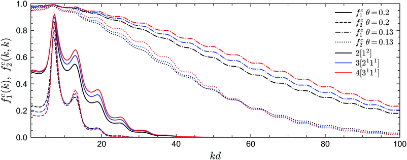
We now turn to the long-time limits of the normalized multi-point density correlation functions, i.e., the non-ergodicity parameters fn(k1,…,kn). We will focus on a very low attractive potential well width of δ = 0.03, for which the sticky hard sphere model exhibits both glass–liquid–glass reentrance and a glass–glass transition. Let us first consider the liquid–glass transition. Fig. 5 shows the critical non-ergodicity parameters fc1(k) and fc2(k,k) at two different temperatures, one at the critical repulsive glass state (θ = 0.2) and the other at the critical attractive glass state (θ = 0.13). It can be seen that the repulsive glass state is similar to the hard-sphere case in the sense that fc1(k) is strongly modulated by the shape of S(k) and the localization length is around the size of one particle diameter.22,58,71,72 Conversely, the non-ergodicity parameters of the attractive glass are much higher than those of the repulsive glass, and they decay to zero over a much wider range of wavenumbers k.58,71,72 This indicates that particle bonding at small distances indeed plays a more important role in the attractive glass phase. Notably, we observe this phenomenology for all considered GMCT closure levels N. Hence, even though higher-order GMCT predicts quantitatively different values of the non-ergodicity parameters, the theory clearly distinguishes between the two types of glasses in a similar manner as standard MCT.Let us further quantify the difference between MCT and higher-order GMCT by careful inspection of Fig. 5. For the lowest-order non-ergodicity parameters fc1(k), we find that increasing N generally leads to an increase in fc1(k), similar to what has been reported previously for GMCT of hard spheres (see Fig. 1 of ref. 23). The only small exception to this N-dependent trend for sticky hard spheres is observed at low temperature (θ = 0.13) and at small wavenumbers kd < 7.4, where k0d = 7.4 corresponds to the first peak of S(k). Overall, at the level of the two-point density correlators, the effect of higher-order GMCT corrections to MCT thus appears to be qualitatively the same for both the attractive and repulsive glass. However, the influence of N on the diagonal four-point density correlators fc2(k, k) is more complex. Indeed, for large wavenumbers k (kd > 15 for θ = 0.2 and kd > 60 for θ = 0.13), fc2(k, k) monotonically decreases with increasing N for both glass types, while for smaller k, the ordering of the fc2(k, k) curves changes under different closure levels. Moreover, the number of such crossovers is different for different temperatures. Hence, in general we can conclude that within GMCT fc2(k, k) ≠ fc1(k) × fc1(k), a result that may hint at the presence of dynamical heterogeneities.
The off-diagonal correlators fc2(k1, k2) at θ = 0.2 and θ = 0.13 are shown in Fig. 6(a) and Fig. 7(a–d), respectively. We find that the pattern of fc2(k1, k2) is qualitatively rather similar for all closure levels N, with a shape that is modulated by S(k). For MCT this shape is in fact trivial since then fc2(k1, k2) = fc1(k1) × fc1(k2); for higher-order GMCT, our repulsive-glass results are also consistent with the GMCT results for hard spheres.21 To see the effect of N for sticky hard spheres more clearly, we plot the difference between fc2(k1, k2) for N > 2 and N = 2 in Fig. 6(b, c) and 7(b, c, e, f). It is clear that as N increases, the GMCT deviations of fc2(k1,k2) with respect to MCT increase both in absolute value and in wavenumber range. However, comparing the results for the repulsive and attractive glass, we see that for the attractive glass phase the deviations extend over a much broader window of wavenumbers. This difference can also be seen if we plot fc2(k1, k2) − fc1(k1) × fc1(k2) for a given state point, i.e. the absolute difference of the four-point non-ergodicity parameters with respect to Gaussian factorization (see the figures in the appendix). We speculate that the difference may stem from the different physical mechanisms, i.e., caging versus bonding, underlying the vitrification process, and it might also point toward different degrees of dynamical heterogeneity in the two glassy phases. This hypothesis, however, still requires further study and should be investigated in future work.
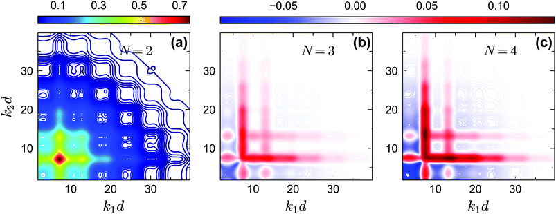 | ||
| Fig. 6 (a) Non-ergodicity parameters fc2(k1, k2) as a function of wavenumbers k1 and k2 at the critical packing fraction for closure level N = 2 (i.e., standard MCT) at θ = 0.2 and δ = 0.03. The patterns of fc2(k1, k2) from N = 3 and N = 4 are similar. (b) The difference of the non-ergodicity parameters fc2(k1, k2) of closure level N = 3 with respect to N = 2. (c) The difference of the non-ergodicity parameters fc2(k1, k2) of closure level N = 4 with respect to N = 2. The packing fractions are the same as in Fig. 5. | ||
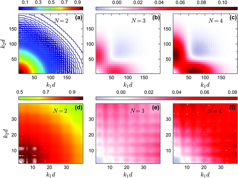 | ||
| Fig. 7 (a) Non-ergodicity parameters fc2(k1, k2) as a function of wavenumbers k1 and k2 at the critical packing fraction for closure level N = 2 (i.e., standard MCT) at θ = 0.13 and δ = 0.03. The patterns of fc2(k1, k2) from N = 3 and N = 4 are similar. (b) The difference of the non-ergodicity parameters fc2(k1, k2) of closure level N = 3 with respect to N = 2. (c) The difference of the non-ergodicity parameters fc2(k1, k2) of closure level N = 4 with respect to N = 2. Panels (d–f) represent the zoomed in small-wavenumber regime of panels (a–c), respectively. The packing fractions are the same as in Fig. 5. | ||
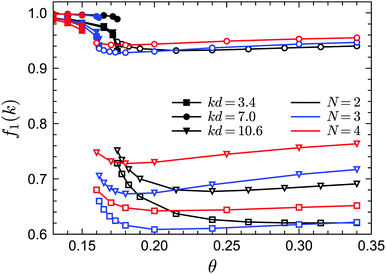
To demonstrate the existence of the glass–glass transition within GMCT, we plot the non-ergodicity parameters f1(k) as a function of θ for different closure levels N. Fig. 8 shows f1(k) for three selected packing fractions and for three representative wavenumbers k; we mention that the wavenumber dependence of f1(k) at both sides of the glass–glass transition line is similar to the result of Fig. 5. For all closure levels N and all considered wavenumbers k, we can see that f1(k) initially decreases as θ increases, until a discontinuous drop occurs; this point corresponds to the A2 singularity of the attractive-to-repulsive-glass transition. In this process, f1(k) follows the same scaling law as eqn (15). As θ further increases within the repulsive glass phase, f1(k) will decrease further for all N (see e.g. the open triangles in Fig. 8). However, after crossing a certain temperature, f1(k) is seen to increase with θ and finally approaches the hard-sphere limit. This effect is essentially the counterpart of the glass–liquid–glass reentrance within the glassy region. The non-trivial variation of f1(k) with θ near but above the critical temperature is a precursor phenomenon of the nearby A3 singularity. Therefore, we conclude that for all GMCT mean-field closure levels N, the glass–glass transition and the A3 singularity are preserved but with quantitatively changed positions in the three-dimension parameter space of sticky hard spheres.
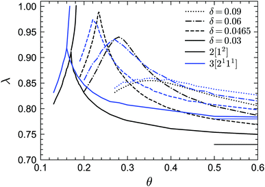
Finally we discuss the exponent parameter λ, which plays a crucial role in the context of Al singularities. Fig. 9 shows λ as a function of θ for the phase transition lines under MF closure levels N = 2 and N = 3. Let us first focus on the standard MCT (N = 2) results. For relative high values of δ, such as δ = 0.09, 0.06, λ shows a single maximum. As δ decreases, the peak value of λ increases and the corresponding position of θ decreases. However, for very small δ, e.g. δ = 0.03, there is another line, representing the glass–glass transition, above the peak. This line ends at the A3 singularity with λ = 1. Therefore there must be a δ between 0.06 and 0.03, which we estimate to be δ ≈ 0.0465, for which the glass–glass transition curve shrinks to zero and the peak lies at λ = 1, which defines the A4 singularity. In fact, the higher-order singularity points shown in Fig. 2 can be found with the guide of the λ curves, as mentioned before. For GMCT with N = 3, the shapes of the λ curves are similar to MCT but quantitatively different. The peak of λ(θ) at δ = 0.0465 for N = 3 is 0.97 ≈ 1, and hence we conjecture the N = 3 A4 point to exist for a δ value close to or slightly lower than 0.0465. From the values of λ when λ < 1, we can also calculate the corresponding exponents a, b and γ by virtue of eqn (19) and (20), i.e., the scaling laws of the relaxation dynamics near A2 singularities. Notice that at large θ, λ must go to the value of the hard-sphere limit, i.e., λ = 0.73 for N = 2 (thin black line in Fig. 9) and λ = 0.78 for N = 3 (thin blue line in Fig. 9), for any value of δ. This puts a physical constraint on possible rescaling approaches; in particular, for fixed δ, the curves of λ(θ) for different closure levels N cannot collapse to one curve by simply shifting θ. This is a further manifestation of the non-trivial effects imposed by higher-order GMCT on the glassy dynamics of sticky hard spheres, consistent with the subtle differences in the phase diagrams of Section 3.1.
In view of the above findings, let us also make a general remark on the rescaling procedure widely used in standard MCT. For sticky hard spheres, it is in a sense accidental that a linear rescaling of only the packing fraction φ and the reduced temperature θ at constant δ has been so successfully applied for the A3 and A4 singularities. The success of this rescaling approach relies on the fact that the shape of φc(θ) near the A3 or A4 singularities and the shape of the peaks of λ(θ) remain very similar under different closure levels N for a given δ. We expect this similarity to continue as N increases until N → ∞. It is this inherent robustness that renders a simple rescaling of θ and φ in MCT sufficient to predict the A3 and A4 singularities within tolerance errors.39 However, regardless of how we rescale φ and θ, it is strictly impossible to merge the full φc(θ) and λ(θ) curves without simultaneously rescaling δ. Consequently, we argue that it is a priori somewhat imprudent to test MCT by only rescaling two parameters; ideally one should first solve the first two or three levels of the GMCT hierarchy to establish a robust trend of the transitions before applying such a rescaling approach.
3.3 Relaxation dynamics
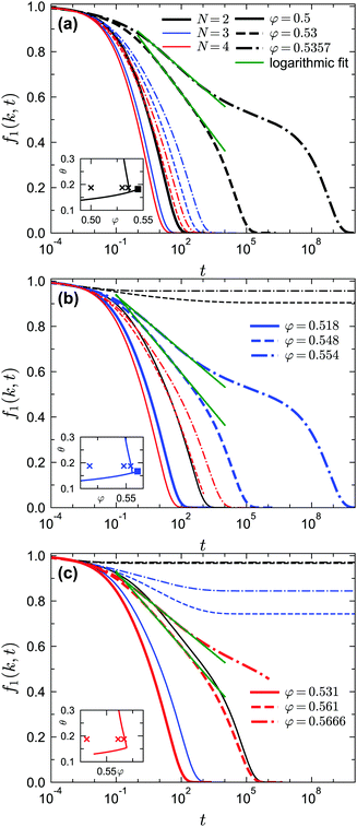
We now consider the time dependence of the dynamic density correlators. The effect of higher-order GMCT on the structural relaxation dynamics of monodisperse hard spheres has already been studied in detail.21–23 As already mentioned in Section 2, one of the conclusions of these recent studies is that for all packing fractions and wavenumbers, GMCT MF closures provide an upper bound to the dynamics while the exponential closures give a lower bound. The two types of closures systematically converge to each other when the closure level N increases. More specifically, if we focus on the MF closures, the predicted relaxation becomes faster in a convergent manner. Here we find that this pattern also applies to sticky hard spheres, i.e., for a given state (fixed packing fraction, fixed reduced temperature, and fixed relative width of the potential well), the relaxation is faster when the MF closure level N increases. We can clearly see this in Fig. 10, where the normalized intermediate scattering functions f1(k, t) = F1(k, t)/S(k) at nine different liquid states under different MF closure levels are presented. For example, it can be seen that the N = 3 results (blue lines in Fig. 10) always decay faster than the corresponding N = 2 (black) curves, and more generally the differences between the curves for closure levels N + 1 and N become smaller as N increases. These findings are thus consistent with a uniform convergent trend of the GMCT hierarchy.The more important properties of the dynamics are the scaling laws in the β- and α-relaxation regimes, since these are widely used for analyzing experimental and simulation data. Within MCT, the scaling laws of eqn (17)–(19) and (22) are known to be applicable for liquid states that lie near the A2 singularities but away from the A3 and A4 singularities. Note that in this case the exponent parameter λ must be smaller than 1, or more strictly λ < 0.9, to ensure that the liquid state is sufficiently far away from the A3 and A4 points. We find that the above scaling laws are also preserved within GMCT under MF closures near the corresponding A2 singularities, i.e., near both the GMCT-predicted liquid-to-repulsive-glass and liquid-to-attractive-glass transitions. This is natural and reasonable given the similar mathematical form of the MCT and GMCT equations. However, when the liquid states are close to the A3 and A4 singularities, the above scaling laws for A2 break down and new behaviors of the relaxation dynamics will appear. Hence we will focus on the dynamics near these higher-order singularities in the following.
We first study the dynamics near the A3 singularities for different GMCT closure levels. The A3 points at δ = 0.03 are (θ ≈ 0.182, φ ≈ 0.545) and (θ ≈ 0.167, φ ≈ 0.56) for N = 2 and N = 3, respectively. Even though we could not accurately determine the location of the A3 point for N = 4 due to limited computing power, we are certain this point must exist and should lie at a φ slightly above 0.57 and a θ slightly above 0.156 for δ = 0.03, since there is an N = 4 glass–glass transition found at φ = 0.57 and θ = 0.156 for δ = 0.03 (see also the non-ergodicity parameters in Fig. 8). For our A3 analysis we fix θ = 0.1875 and select three liquid states with different packing fractions for each closure level N; this value of θ is close to the θ of the A3 singularity for all considered N. The results for the predicted normalized dynamical two-point density correlation functions f1(k, t) are shown in Fig. 10. As we get closer to the A3 singularities, we find that the relaxation of f1(k, t) becomes more stretched compared to the power laws described in eqn (18) and (19), and instead a logarithmic relaxation regime appears. This logarithmic decay of f1(k, t) for liquid states near A3 singularities, described viaeqn (23), is applicable for all closure levels N (see the green dashed fitted curves in Fig. 10). The logarithmic law for f1(k, t) near A3 singularities within GMCT qualitatively agrees with the one in MCT, and hence our GMCT results also agree with the body of simulation and experimental data that have already been qualitatively compared to MCT.36,39,49 More generally, we find that higher-order GMCT inherits all the main qualitative features of the MCT dynamics near A3 singularities. In particular, upon approaching the A3 point from the liquid side (black, blue, and red dashed lines in Fig. 10(a), (b), and (c), respectively), we can also see that the α-relaxation process does not start with von Schweidler law of eqn (19), and as a consequence the superposition principle of eqn (22) is disobeyed.58 The only main difference between MCT and GMCT is that the corresponding packing fractions are improved, since the A3 point becomes more accurate upon increasing the closure level.
Besides the logarithmic decay for f1(k, t), we find that this logarithmic decay is also applicable for 2n-point density correlation functions with n > 1. For example, in Fig. 11 we show f2(k, k, t) near the A3 singularity under closure level N = 3 for two different wavenumbers. The fit with f2(k, k, t) = fc2(k, k) − C2(k, k)![[thin space (1/6-em)]](https://www.rsc.org/images/entities/char_2009.gif) ln(t), where C2(k, k) is a wavenumber-dependent constant, is applicable for more than three decades in time. To the best of our knowledge, no empirical results for f2(k, k, t) or similar higher-order dynamical density correlation functions have been reported in this glassy regime. We argue that the logarithmic decay for higher-order correlators can be another strict test for both GMCT and the A3 singularities predicted from it for sticky hard spheres.
ln(t), where C2(k, k) is a wavenumber-dependent constant, is applicable for more than three decades in time. To the best of our knowledge, no empirical results for f2(k, k, t) or similar higher-order dynamical density correlation functions have been reported in this glassy regime. We argue that the logarithmic decay for higher-order correlators can be another strict test for both GMCT and the A3 singularities predicted from it for sticky hard spheres.
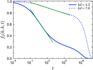 | ||
Fig. 11 Normalized four-point density correlation functions f2(k, k, t) for liquid states at δ = 0.03, θ = 0.1875 and φ = 0.554 (corresponding to the right cross in the inset of Fig. 10(b)) near the A3 singularities predicted from GMCT with closure level N = 3. The solid and dotted curves correspond to wavenumber k = 4.2 and k = 7.0, respectively. The green lines are fits to the expression f2(k, k, t) = fc2(k, k) − C2(k, k)![[thin space (1/6-em)]](https://www.rsc.org/images/entities/char_2009.gif) ln(t), where C2(k, k) is a wavenumber-dependent constant. ln(t), where C2(k, k) is a wavenumber-dependent constant. | ||
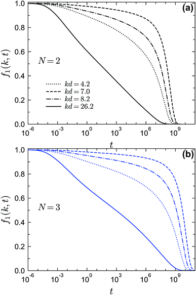
Finally let us go to the dynamics of the density correlation functions near the A4 singularities. The regime of the very stretched and nearly logarithmic decay of f1(k, t) is found for both closure levels N = 2 and N = 3, as indicated by the solid lines in Fig. 12. The range of this regime can be much wider than the range near A3 in Fig. 10, although for N = 3 [blue solid line in Fig. 12(b)] the range of the strictly logarithmic decay is not as wide as the one for N = 2 [black solid line in Fig. 12(a)]. We attribute this to the lower numerical accuracy of the A4 singularity for N = 3 (with a maximum λ = 0.97 at δ = 0.0465 instead of λ = 1). We have also verified that the logarithmic decay is found for f2(k1, k2, t) at several wavenumbers (not shown here). We further test the time-wavenumber factorization property, eqn (17), near the A4 singularities. If the factorization property holds, the rescaled correlation functions [fn(k1,…,kn,t) − fcn(k1,…,kn)]/hn(k1,…,kn) should collapse on the common function G(t). In particular, all correlators should cross their plateau value fcn(k1,…,kn, t) at the same time t− with G(t−) = 0. We show the rescaled correlation function of f1(k, t) in Fig. 13(a) with the fc1(k) and h1(k) [shown in Fig. 13(b)] from the A4 singularity point under the corresponding closure level N. We find that for both N = 2 and N = 3, the factorization property is still satisfied (see Fig. 13(a) with the arrows indicating the t−). However, the validity range is only around two decades in time, which is much narrower than the one near A2 singularities, for which the factorization property applies over approximately four decades.22,58
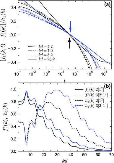 | ||
| Fig. 13 Scaling laws near the A4 singularity point. (a) Rescaled two-point density correlation functions [f1(k, t) − fc1(k)]/h1(k) at the same liquid states as in Fig. 12, i.e., near the corresponding A4 points for GMCT closure levels N = 2 (black lines) and N = 3 (blue lines). The black (blue) arrow indicates the position of G(t−) = 0 with t− = 1.48 × 10³ (t− = 1.95 × 10³) for closure level N = 2 (N = 3). (b) The functions fc1(k) and h1(k) obtained from the corresponding A4 singularities using eqn (8) and (16). | ||
4 Conclusion
In this work, we have presented a detailed numerical analysis of the glassy dynamics of sticky hard spheres using first-principles-based microscopic generalized mode-coupling theory. We have obtained the phase diagrams in the three-dimensional control-parameter space under different mean-field closure levels in GMCT. Upon increasing the closure level N of the GMCT hierarchy, i.e., by expanding the dynamical equations in terms of increasingly higher order density correlations, the phase diagrams become closer to the empirical results. We have clarified that the improvement from GMCT is not merely a simple rescaling of control parameters, as is usually done in standard MCT analyses; rather, higher-order GMCT yields subtle but intrinsically different results compared to MCT, as reflected in the shifted phase diagrams of sticky hard spheres relative to the hard-sphere case, and the exponent parameter λ.From the phase diagrams and the non-ergodicity parameters, we have demonstrated that the peculiar features of dense sticky hard spheres, i.e., glassy reentrance, a glass–glass transition, and higher-order A3 and A4 singularities, are also successfully predicted from GMCT. The positions of these transition points are also more accurate than those obtained from standard MCT. These triumphs indicate that the complex interplay of repulsive and attractive short-ranged interactions can be adequately captured within GMCT. We have also demonstrated that when the attraction is very strong, the difference of the predicted critical packing fractions at any given width of the potential well between GMCT and MCT becomes much larger. This implies that, compared to repulsive interactions, the attractive part of the interaction potential may play a more important role in the higher-order density correlation functions. This non-trivial effect of attractions has also been reflected in the different patterns of the non-ergodicity parameters of the four-point density correlation functions fc2(k1, k2) for the repulsive-glass and attractive-glass phase. We hypothesize that these higher-order density correlations may also contain new, and non-trivial, information on dynamical heterogeneity,43 but further research is needed to clarify their precise physical interpretation.
Within higher-order GMCT, we have shown that the celebrated scaling laws for A2 singularities are no longer applicable when the considered state point is in the vicinity of an A3 or A4 singularity. In that case, we find a logarithmic decay in the dynamics that is consistent with the MCT form of eqn (23). We emphasize, however, that this logarithmic decay is applicable not only for the conventionally studied intermediate scattering function f1(k, t), but also for higher-order density correlation functions such as f2(k, k, t). The latter of course needs to be further verified in simulations or experiments.
From all the results above, we conclude that GMCT can make detailed first-principles-based predictions of the microscopic dynamics of sticky hard spheres well beyond the standard-MCT regime, whilst maintaining many of the qualitative features of MCT. Interestingly, although a significant body of experimental47–51,56 and simulation35–44 work has corroborated the qualitative MCT scenario for sticky hard spheres,35–41 a recent swap Monte Carlo simulation57 disputes the existence of the MCT-predicted liquid–glass transition, the glass–glass transition, and all the higher-order Al singularities, claiming that these MCT-predicted phenomena in fact lie within a unique ergodic region. Our results support this conclusion in the sense that the MCT-predicted glass transitions are shifted toward higher packing fractions within higher-order GMCT, and as N increases they might become close to or even higher than the highest packing fractions accessible in simulation. However, we here argue that the liquid–glass transition, glass–glass transition and higher-order singularities could still exist, possibly at even higher packing fractions than those probed by state-of-the-art simulations.57 We also emphasize that our theoretical results are based on a monodisperse sticky hard sphere model, while the swap Monte Carlo simulations of ref. 57 assume a relatively large polydispersity of 23%. It is known in general that polydispersity can significantly affect the glassy dynamics and the corresponding phase diagrams,73 and hence this aspect should be also carefully studied in future work. Finally, the high-order singularities and logarithmic relaxation of sticky hard spheres may also have a deep analogy to the glassy behavior of randomly pinned supercooled liquids and that of the random field Ising model, as discovered within the inhomogeneous MCT.74 We believe this analogy would also be preserved in our GMCT framework, although further work on this is needed.
Since the sticky hard sphere model contains both attractive and repulsive interactions, we may expect that GMCT is also a suitable framework for other systems with short-ranged attractive interactions. It remains to be explored, however, whether the current GMCT framework can ultimately provide a universal description of the elusive structure-dynamics link in glass-forming materials. Firstly, there are still some subtle approximations in our current theory, such as the diagonal approximation for the dynamical higher-order density correlation functions in the GMCT memory functions,60 and the Gaussian factorization and convolution approximation for all higher-order static density correlation functions.19,21 Recent studies suggest that higher-order and local structural metrics also encode rich physics and contribute to the dynamics in a non-trivial manner,6,18,75 but these structural quantities are all simply regarded as being implicitly included in S(k) or neglected in the current GMCT framework. Future work will be done to test how accurate these approximations are and how one might admit more detailed structural information into the theory. Second, until now, GMCT has been tested only for systems with purely repulsive or repulsive with short-ranged attractive isotropic potentials. These systems all belong to the class of fragile glass formers.76,77 More work needs be done to test GMCT for strong glass formers such as silica14, or even superstrong systems such as vitrimers.33
Conflicts of interest
There are no conflicts to declare.Appendix: breakdown of Gaussian factorization for attractive and repulsive glasses
In Fig. 14 and 15, we plot the off-diagonal non-ergodicity parameters fc2(k1, k2) and the difference fc2(k1, k2) − fc1(k1) ×fc1(k2) at the critical liquid–glass transition points for θ = 0.2 and θ = 0.13 at δ = 0.03 under GMCT closure levels N = 2, 3, and 4. The patterns of fc2(k1, k2) −fc1(k1) × fc1(k2) for the repulsive glass (Fig. 14(b and c)) and the attractive glass (Fig. 15(b, c, e and f)) are very different. Overall these results support the fact that Gaussian factorization can both overestimate and underestimate the four-point non-ergodicity parameters in certain wavenumber regimes, and the deviation pattern depends on the type of glass state.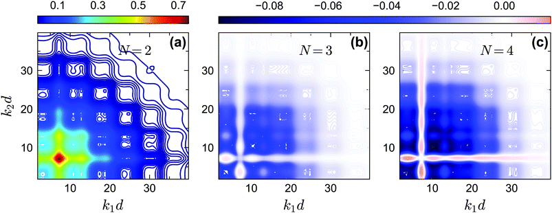 | ||
| Fig. 14 (a) The non-ergodicity parameters fc2(k1,k2) as a function of wavenumbers k1 and k2 at the critical packing fraction for closure level N = 2 (i.e., standard MCT) at θ = 0.2. The patterns of fc2(k1, k2) from N = 3 and N = 4 are similar. (b) The difference of the non-ergodicity parameters f2c(k1,k2) of closure level N = 3 with respect to the factorization approximation fc1(k1) × fc1(k2) at the same state. (c) Same as in (b) but for N = 4. The packing fractions are the same as in Fig. 5. | ||
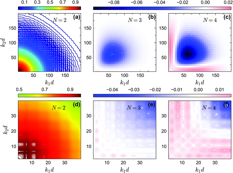 | ||
| Fig. 15 (a) The non-ergodicity parameters fc2(k1, k2) as a function of wavenumbers k1 and k2 at the critical packing fraction for closure level N = 2 (i.e., standard MCT) at θ = 0.13. The patterns of fc2(k1, k2) from N = 3 and N = 4 are similar. (b) The difference of the non-ergodicity parameters fc2(k1, k2) of closure level N = 3 with respect to the factorization approximation fc1(k1) × fc1(k2) at the same state. (c) Same as in (b) but for N = 4. Panels (d–f) contain the same data as panels (a–c), respectively, but are enlarged for small wavenumbers. The packing fractions are the same as in Fig. 5. | ||
Acknowledgements
We acknowledge the Netherlands Organisation for Scientific Research (NWO) for financial support through a START-UP grant.Notes and references
- P. G. Debenedetti and F. H. Stillinger, Nature, 2001, 410, 259 CrossRef CAS PubMed.
- L. Berthier and G. Biroli, Rev. Mod. Phys., 2011, 83, 587 CrossRef CAS.
- W. Götze, Complex dynamics of glass-forming liquids: A Mode-Coupling Theory, Oxford University Press, Oxford, 2009 Search PubMed.
- G. Tarjus, S. A. Kivelson, Z. Nussinov and P. Viot, J. Phys.: Condens. Matter, 2005, 17, R1143 CrossRef CAS.
- T. Kirkpatrick and D. Thirumalai, Rev. Mod. Phys., 2015, 87, 183 CrossRef CAS.
- H. Liu, Z. Fu, K. Yang, X. Xu and M. Bauchy, J. Non-Cryst. Solids, 2019, 119419 Search PubMed.
- X. Ma, Z. S. Davidson, T. Still, R. J. Ivancic, S. Schoenholz, A. Liu and A. Yodh, Phys. Rev. Lett., 2019, 122, 028001 CrossRef CAS PubMed.
- S. S. Schoenholz, E. D. Cubuk, D. M. Sussman, E. Kaxiras and A. J. Liu, Nat. Phys., 2016, 12, 469–471 Search PubMed.
- V. Bapst, T. Keck, A. Grabska-Barwińska, C. Donner, E. D. Cubuk, S. S. Schoenholz, A. Obika, A. W. Nelson, T. Back and D. Hassabis, et al. , Nat. Phys., 2020, 16, 448–454 Search PubMed.
- U. Bengtzelius, W. Götze and A. Sjolander, J. Phys. C: Solid State Phys., 1984, 17, 5915 CrossRef CAS.
- E. Leutheusser, Phys. Rev. A: At., Mol., Opt. Phys., 1984, 29, 2765 CrossRef CAS.
- D. R. Reichman and P. Charbonneau, J. Stat. Mech.: Theor. Exp., 2005, P05013 Search PubMed.
- L. M. C. Janssen, Front. Phys., 2018, 6, 97 CrossRef.
- F. Sciortino and W. Kob, Phys. Rev. Lett., 2001, 86, 648 CrossRef CAS.
- W. Kob, C. Donati, S. J. Plimpton, P. H. Poole and S. C. Glotzer, Phys. Rev. Lett., 1997, 79, 2827 CrossRef CAS.
- S. C. Glotzer, V. N. Novikov and T. B. Schrøder, J. Chem. Phys., 2000, 112, 509–512 CrossRef CAS.
- N. Lačević, F. W. Starr, T. Schrøder and S. Glotzer, J. Chem. Phys., 2003, 119, 7372–7387 CrossRef.
- Z. Zhang and W. Kob, Proc. Natl. Acad. Sci. U. S. A., 2020, 117, 14032–14037 CrossRef CAS PubMed.
- G. Szamel, Phys. Rev. Lett., 2003, 90, 228301 CrossRef.
- J. Wu and J. Cao, Phys. Rev. Lett., 2005, 95, 078301 CrossRef PubMed.
- L. M. C. Janssen and D. R. Reichman, Phys. Rev. Lett., 2015, 115, 205701 CrossRef.
- C. Luo and L. M. C. Janssen, J. Chem. Phys., 2020, 153, 214507 CrossRef CAS PubMed.
- C. Luo and L. M. C. Janssen, J. Chem. Phys., 2020, 153, 214506 CrossRef CAS PubMed.
- W. Kob and H. C. Andersen, Phys. Rev. E: Stat. Phys., Plasmas, Fluids, Relat. Interdiscip. Top., 1995, 52, 4134 CrossRef CAS PubMed.
- L. Berthier and G. Tarjus, Phys. Rev. E: Stat., Nonlinear, Soft Matter Phys., 2010, 82, 031502 CrossRef PubMed.
- V. Zöllmer, K. Rätzke, F. Faupel and A. Meyer, Phys. Rev. Lett., 2003, 90, 195502 CrossRef PubMed.
- B. Nowak, D. Holland-Moritz, F. Yang, T. Voigtmann, T. Kordel, T. Hansen and A. Meyer, Phys. Rev. Mater., 2017, 1, 025603 CrossRef.
- G. Szamel and H. Löwen, Phys. Rev. A: At., Mol., Opt. Phys., 1991, 44, 8215 CrossRef CAS.
- M. Siebenbürger, M. Fuchs, H. Winter and M. Ballauff, J. Rheol., 2009, 53, 707–726 CrossRef.
- L. Schrack and T. Franosch, Philos. Mag., 2020, 100, 1032–1057 CrossRef CAS PubMed.
- J. Farago, A. Semenov, H. Meyer, J. Wittmer, A. Johner and J. Baschnagel, Phys. Rev. E: Stat., Nonlinear, Soft Matter Phys., 2012, 85, 051806 CrossRef CAS PubMed.
- J. Farago, H. Meyer, J. Baschnagel and A. Semenov, Phys. Rev. E: Stat., Nonlinear, Soft Matter Phys., 2012, 85, 051807 CrossRef CAS PubMed.
- S. Ciarella, R. A. Biezemans and L. M. C. Janssen, Proc. Natl. Acad. Sci. U. S. A., 2019, 116, 25013–25022 CrossRef CAS.
- C. Ruscher, S. Ciarella, C. Luo, L. M. C. Janssen, J. Farago and J. Baschnagel, J. Phys.: Condens. Matter, 2020, 33, 064001 CrossRef.
- A. M. Puertas, M. Fuchs and M. E. Cates, Phys. Rev. Lett., 2002, 88, 098301 CrossRef PubMed.
- E. Zaccarelli, G. Foffi, K. A. Dawson, S. Buldyrev, F. Sciortino and P. Tartaglia, Phys. Rev. E: Stat., Nonlinear, Soft Matter Phys., 2002, 66, 041402 CrossRef CAS.
- G. Foffi, K. A. Dawson, S. V. Buldyrev, F. Sciortino, E. Zaccarelli and P. Tartaglia, Phys. Rev. E: Stat., Nonlinear, Soft Matter Phys., 2002, 65, 050802 CrossRef CAS PubMed.
- E. Zaccarelli, G. Foffi, F. Sciortino and P. Tartaglia, Phys. Rev. Lett., 2003, 91, 108301 CrossRef PubMed.
- F. Sciortino, P. Tartaglia and E. Zaccarelli, Phys. Rev. Lett., 2003, 91, 268301 CrossRef.
- E. Zaccarelli, F. Sciortino and P. Tartaglia, J. Phys.: Condens. Matter, 2004, 16, S4849 CrossRef CAS.
- G. Foffi, F. Sciortino, E. Zaccarelli and P. Tartaglia, J. Phys.: Condens. Matter, 2004, 16, S3791 CrossRef CAS.
- I. Saika-Voivod, E. Zaccarelli, F. Sciortino, S. V. Buldyrev and P. Tartaglia, Phys. Rev. E: Stat., Nonlinear, Soft Matter Phys., 2004, 70, 041401 CrossRef CAS PubMed.
- D. R. Reichman, E. Rabani and P. L. Geissler, J. Phys. Chem. B, 2005, 109, 14654–14658 CrossRef CAS PubMed.
- A. J. Moreno and J. Colmenero, Phys. Rev. E: Stat., Nonlinear, Soft Matter Phys., 2006, 74, 021409 CrossRef PubMed.
- K. González-López, M. Shivam, Y. Zheng, M. P. Ciamarra and E. Lerner, Phys. Rev. E, 2021, 103, 022605 CrossRef.
- K. González-López, M. Shivam, Y. Zheng, M. P. Ciamarra and E. Lerner, Phys. Rev. E, 2021, 103, 022606 CrossRef.
- F. Mallamace, P. Gambadauro, N. Micali, P. Tartaglia, C. Liao and S.-H. Chen, Phys. Rev. Lett., 2000, 84, 5431 CrossRef CAS.
- T. Eckert and E. Bartsch, Phys. Rev. Lett., 2002, 89, 125701 CrossRef CAS.
- K. N. Pham, A. M. Puertas, J. Bergenholtz, S. U. Egelhaaf, A. Moussad, P. N. Pusey, A. B. Schofield, M. E. Cates, M. Fuchs and W. C. Poon, Science, 2002, 296, 104–106 CrossRef CAS PubMed.
- K. Pham, S. Egelhaaf, P. Pusey and W. C. Poon, Phys. Rev. E: Stat., Nonlinear, Soft Matter Phys., 2004, 69, 011503 CrossRef CAS PubMed.
- L. J. Kaufman and D. A. Weitz, J. Chem. Phys., 2006, 125, 074716 CrossRef.
- S. Buzzaccaro, R. Rusconi and R. Piazza, Phys. Rev. Lett., 2007, 99, 098301 CrossRef.
- P. J. Lu, E. Zaccarelli, F. Ciulla, A. B. Schofield, F. Sciortino and D. A. Weitz, Nature, 2008, 453, 499–503 CrossRef CAS PubMed.
- Z. Zhang, P. J. Yunker, P. Habdas and A. Yodh, Phys. Rev. Lett., 2011, 107, 208303 CrossRef PubMed.
- Z. Brown, M. J. Iwanicki, M. D. Gratale, X. Ma, A. Yodh and P. Habdas, EPL, 2016, 115, 68003 CrossRef.
- N. Willenbacher, J. S. Vesaratchanon, O. Thorwarth and E. Bartsch, Soft Matter, 2011, 7(12), 5777–5788 RSC.
- C. J. Fullerton and L. Berthier, Phys. Rev. Lett., 2020, 125, 258004 CrossRef CAS PubMed.
- K. Dawson, G. Foffi, M. Fuchs, W. Götze, F. Sciortino, M. Sperl, P. Tartaglia, T. Voigtmann and E. Zaccarelli, Phys. Rev. E: Stat. Phys., Plasmas, Fluids, Relat. Interdiscip. Top., 2000, 63, 011401 CrossRef.
- J.-P. Hansen and I. R. McDonald, Theory of simple liquids, Elsevier, Amsterdam, 2013 Search PubMed.
- S. Ciarella, PhD thesis, Eindhoven University of Technology, 2021.
- R. Zwanzig, Nonequilibrium statistical mechanics, Oxford University Press, 2001 Search PubMed.
- L. M. C. Janssen, P. Mayer and D. R. Reichman, J. Stat. Mech.: Theor. Exp., 2016, 054049 CrossRef.
- R. A. Biezemans, S. Ciarella, O. Çaylak, B. Baumeier and L. M. C. Janssen, J. Stat. Mech.: Theor. Exp., 2020, 103301 CrossRef.
- C. D. Meyer, Matrix analysis and applied linear algebra, Siam, 2000, vol. 71 Search PubMed.
- V. I. Arnol'd, Catastrophe theory, Springer Science & Business Media, 2003 Search PubMed.
- W. Gotze and L. Sjogren, J. Phys.: Condens. Matter, 1989, 1, 4203 CrossRef.
- W. Götze and M. Sperl, Phys. Rev. E: Stat., Nonlinear, Soft Matter Phys., 2002, 66, 011405 CrossRef PubMed.
- T. Franosch, M. Fuchs, W. Götze, M. R. Mayr and A. Singh, Phys. Rev. E: Stat. Phys., Plasmas, Fluids, Relat. Interdiscip. Top., 1997, 55, 7153 CrossRef CAS.
- M. Fuchs, W. Gotze, I. Hofacker and A. Latz, J. Phys.: Condens. Matter, 1991, 3, 5047 CrossRef.
- W. Götze and M. Sperl, J. Phys.: Condens. Matter, 2003, 15, S869 CrossRef.
- L. Fabbian, W. Götze, F. Sciortino, P. Tartaglia and F. Thiery, Phys. Rev. E: Stat. Phys., Plasmas, Fluids, Relat. Interdiscip. Top., 1999, 59, R1347 CrossRef CAS.
- J. Bergenholtz and M. Fuchs, Phys. Rev. E: Stat. Phys., Plasmas, Fluids, Relat. Interdiscip. Top., 1999, 59, 5706 CrossRef CAS PubMed.
- S. Ciarella, C. Luo, V. E. Debets and L. Janssen, 2021, arXiv preprint arXiv:2103.16522.
- S. K. Nandi, G. Biroli, J.-P. Bouchaud, K. Miyazaki and D. R. Reichman, Phys. Rev. Lett., 2014, 113, 245701 CrossRef.
- J. F. Robinson, F. Turci, R. Roth and C. P. Royall, Phys. Rev. Lett., 2019, 122, 068004 CrossRef CAS PubMed.
- T. Scopigno, G. Ruocco, F. Sette and G. Monaco, Science, 2003, 302, 849–852 CrossRef CAS.
- L.-M. Martinez and C. Angell, Nature, 2001, 410, 663–667 CrossRef CAS.
| This journal is © The Royal Society of Chemistry 2021 |


