
 Open Access Article
 This Open Access Article is licensed under a
 Creative Commons Attribution 3.0 Unported Licence
Insights from modeling into structure, entanglements, and dynamics in attractive polymer nanocomposites†
Ahmad
Moghimikheirabadi
 *a,
Martin
Kröger
*a and
Argyrios V.
Karatrantos
*b
*a,
Martin
Kröger
*a and
Argyrios V.
Karatrantos
*b
aDepartment of Materials, Polymer Physics, ETH Zurich, Leopold-Ruzicka-Weg 4, CH-8093 Zurich, Switzerland. E-mail: ahmadm@mat.ethz.ch; mk@mat.ethz.ch
bMaterials Research and Technology, Luxembourg Institute of Science and Technology, 5, Avenue des Hauts-Fourneaux, L-4362 Esch-sur-Alzette, Luxembourg. E-mail: argyrios.karatrantos@list.lu
First published on 9th June 2021
Abstract
Conformations, entanglements and dynamics in attractive polymer nanocomposites are investigated in this work by means of coarse-grained molecular dynamics simulation, for both weak and strong confinements, in the presence of nanoparticles (NPs) at NP volume fractions ϕ up to 60%. We show that the behavior of the apparent tube diameter dapp in such nanocomposites can be greatly different from nanocomposites with nonattractive interactions. We find that this effect originates, based on a mean field argument, from the geometric confinement length dgeo at strong confinement (large ϕ) and not from the bound polymer layer on NPs (interparticle distance ID <2Rg) as proposed recently based on experimental measurements. Close to the NP surface, the entangled polymer mobility is reduced in attractive nanocomposites but still faster than the NP mobility for volume fractions beyond 20%. Furthermore, entangled polymer dynamics is hindered dramatically by the strong confinement created by NPs. For the first time using simulations, we show that the entangled polymer conformation, characterized by the polymer radius of gyration Rg and form factor, remains basically unperturbed by the presence of NPs up to the highest volume fractions studied, in agreement with various experiments on attractive nanocomposites. As a side-result we demonstrate that the loose concept of ID can be made a microscopically well defined quantity using the mean pore size of the NP arrangement.
1 Introduction
The proper dispersion of nanofillers in a polymer matrix is a prerequisite in the diverse attempts to improve the properties of a base polymer material.1 One possible way to achieve a good dispersion and distribution of nanoparticles (NPs) is to make use of polymers and NPs that are mutually attractive. Attractive polymer nanocomposites are often identified by the effective attractive interaction between polymer matrix and NPs which results in the miscibility and homogeneous dispersion of NPs within the polymer matrix. The dispersion state of the NPs and hence the effective attraction can be expressed in terms of the polymer–NP Flory–Huggins interaction parameter χp–NP, that is required to be χp–NP < 0.5 to avoid (micro)phase separation. This interaction parameter χp–NP is available from experimental measurements of the mixing free energy as well as molecular dynamics simulations utilizing thermodynamic integration.2 For nanocomposites containing carbon nanotubes, χp–NP had been calculated from the square of pure-component solubility parameters for many different polymers.3 An effective attraction4 can originate either from hydrogen bonds,5–20 π–π stacking21–24 and ionic25–32 or other types of interaction.23,33–36 The addition of NPs alters polymer rheology,37–41 which affects transport42,43 and flow.44–46 Polymer nanocomposites with very high NP loadings offer a lot of applications in energy storage, or as membrane or coatings, however they are still difficult to be prepared due to poor processability.47,48 As the addition of NPs furthermore influences polymer dynamics (diffusion, reorientation),49–52 a fundamental understanding of the system's dynamics allows for the improvement and design of polymer processing conditions.53 Despite the progress made so far, the existing studies were not able to univocally answer important questions related to conformational and dynamical aspects within such systems.It remained unclear whether the addition of NPs (at any amounts) to a polymer matrix alters the polymer conformations, although this issue has been addressed in several previous, mostly experimental, works.17,33,54–69 Knowledge about the polymer conformation is essential to conclude about the existence of internal stresses, the interconnectivity of the network of chains and NPs, and to estimate characteristic relaxation times that affect various material properties. In particular, there is evidence for unperturbed conformational chain behavior, by small angle neutron scattering (SANS), of an athermal system comprising polystyrene (PS) chains and dispersed nanosilicas.60,70 In those studies, the polymer radius of gyration Rg exceeded the NP radius RNP by a factor between 1.9 and 3.9.60 A similar conclusion was drawn for nanocomposites exhibiting a smaller ratio (Rg/RNP = 0.98–2.13), again using SANS, containing polymers and NPs that attract each other, such as poly(methyl methacrylate) (PMMA) chains and nanosilicas17 or syndiotactic s-PMMA chains and polyhedral oligomeric silsesquioxane (POSS) (Rg/RNP = 10–20).59 Unperturbed dimensions were also found for an attractive poly(ethylene oxide) (PEO)–nanosilica composite with an even smaller ratio (Rg/RNP = 0.28),71 at large NP volume fractions of up to ϕ = 53%.72 In contrast, PS chains were found to expand by up to 20% in the presence of PS-crosslinked NPs (for ratios Rg/RNP = 1.6–5.7)55 or carbon nanotubes.58 A dramatic expansion of polymers by almost 60% at high loading was observed for poly(dimethyl siloxane) (PDMS) in the presence of soft polysilicate RNP = 1 nm NPs (ratios Rg/RNP = 6–8).56,57
Not only the static aspects remain an open issue when NPs are added, but so do the dynamical quantities. Such include relaxation times required to predict the rheological behavior or more generally, the response to external fields, as well as diffusion rates that affect polymer processing conditions. In a series of works, Gam et al.73,74 observed a decrease in the polymer diffusion coefficient as the NP volume fraction for athermal polystyrene/silica nanocomposites increased. Moreover, the tube diameter, characterizing dynamical aspects of entangled polymer matrices, was found to increase with NP loading from neutron spin echo measurements on nanosilica/PEP composites (which can be considered as nanocomposites with nonattractive interactions).75 In attractive PEO–nanosilica nanocomposites, however, a different behavior on the tube diameter was observed recently by Senses et al.72 Furthermore, for a strongly attractive nanocomposite material such as poly(2-vinylpyridine) (P2VP) polymers and nanosilicas, weakly adsorbed chains eventually desorbed from the NP surface, while strongly adsorbed chains remained bound for experimental time scales available to elastic recoil recovery (ERD) and Rutherford Backscattering spectrometry (RBS).76 The bound-layer thickness was found up to Rg/2 distance from the NP surface and was affected by the strength of attraction.12,76–78
Several simulation efforts have tried to explore selected static and dynamic features. Most of them have focused on either a very dilute5,52,54,79–89 or rather moderate NP volume fractions (ϕ < 25%)54,68,90–95 except the Monte Carlo work by Sharaf and Mark96 for a dense athermal system, in which the polymer chains were significantly confined between the NPs and conformations were addressed. In addition, the work by Lin et al.97 focused on the mechanical enhancement under tensile deformation for very high NP loadings. Coarse-grained models for NP/polymer mixtures have revealed that polymers tend to expand with increasing ϕ for relatively small NPs and certain volume fractions,23,68,96,98 as long as 2RNP < Rg and that there was also an attractive interaction between NPs and polymers.66,84,87,98,99 This result was in agreement with the simulation effort in athermal nanocomposites,68,91,96,100 where it was shown that the tube diameter increased with NP loading beyond ϕ = 20%, whereas at low loading, it remained constant,100 in agreement with the above-mentioned experimental observations.75 Another study showed that the disentanglement of chains was enhanced when small NPs were dispersed in the polymer matrix (up to ϕ ≈ 27%) due to the larger confinement and expansion of chains.90 In addition, polymer dynamics has been studied by simulations either of short chains82,83,86,101–104 or at a low NP loading.82,83,86,88
However, there has not yet been any computational effort to address entangled polymer conformations, entanglements and dynamics simultaneously in attractive nanocomposites from low to very high NP loading (ϕ > 40%). The present works aims at closing this gap and developing a picture that captures both static and dynamic aspects of both the NPs and the polymers, from dilute to extreme loadings. After presenting the model and methodology (Section 2), we focus on shedding light on the (i) polymer structure, (ii) entanglements and (iii) dynamics in attractive nanocomposites up to a very high NP loading. To this end, we first explore how spherical NPs, whose diameter is to the order of, or larger than Rg, affect polymer dimensions (Section 3.1), as characterized by the radius of gyration and form factor, and then compare this to experimental measurements (Section 3.2). Secondly, we calculate and evaluate polymer and NP dynamics for different NP loadings, while focusing on the bound layer which affects dynamic properties and reinforcement105–107 (Section 3.3). Thirdly, we investigate the entanglement network for different NP loadings in an attempt to address open questions formulated earlier by Senses et al.72 for attractive nanocomposites (Section 3.4). While Senses claimed that the bound layer is responsible for a constant dapp at high ϕ, we find a behavior that originated, based on a mean field assumption, wholly from the geometrical confinement.78,108 Conclusions are offered in Section 4.
2 Model and methodology
We use a coarse-grained model that is known to capture the relevant dynamics and structure of simple hybrid polymer/nanoparticle systems. Our systems are composed of spherical NPs having beads on the surface and multibead-spring linear polymer chains with N = 100 or N = 200 monomers (Kremer–Grest model109), where each bead represents a number of monomers.110,111 Adjacent beads within chains are connected by anharmonic springs, while the impenetrable NPs are modeled as rigid, mobile objects whose surfaces are covered by surface beads.112 We use Lennard–Jones (LJ) reduced units throughout this manuscript.To be more specific, adjacent beads i and j separated by a spatial distance rij within polymer chains are connected using finitely extensible nonlinear elastic (FENE) springs109,113–117
 | (1) |
 | (2) |
A simulation snapshot of a system with NP volume fraction of ϕ = 30% is shown in Fig. 1. All simulations were started from random distribution of NPs configurations of nanocomposites98 at pressure P = 4.84 and temperature T = 1 for a duration of 5 × 10⁴ LJ time units. Subsequently, NVT ensemble simulations were performed, for a duration of 5 × 10⁵, at T = 1 by means of a Nosé–Hoover thermostat with a damping time of 0.4.117,121 Finally, NVT production runs were performed at T = 1 for another 5 × 10⁵ time units. Due to the choice of the FENE parameters, cutoff, and temperature, the mean bond length is b0 ≈ 1. The linear size of the simulation cell was chosen larger than the root mean square end-to-end distance of the polymer in each case. An integration time step equal to Δt = 0.005 was used for polymer melts and nanocomposites. The molecular dynamics simulations were performed using the LAMMPS package.122
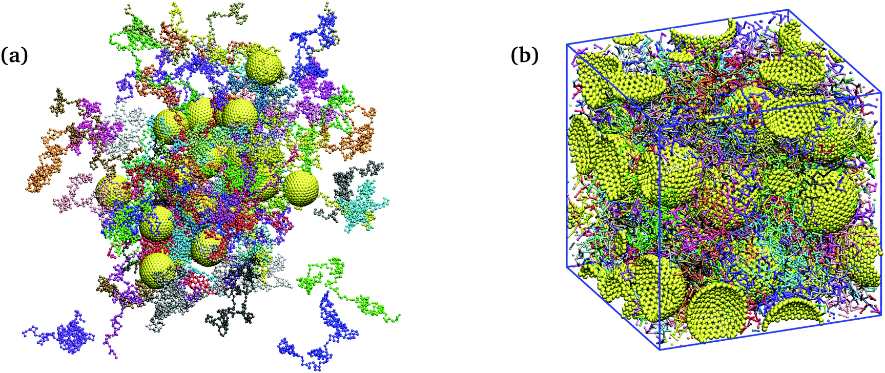 | ||
| Fig. 1 Simulation snapshots. Unwrapped (a), and wrapped (b) coordinates of an attractive polymer nanocomposite at NP volume fraction of ϕ = 30%, consisting of 24 NPs (golden spheres) and 72 polymer chains (colorful beads, N = 200 beads per chain) in a cubic simulation box with the dimensions 28.34 × 28.34 × 28.34. | ||
3 Results and discussion
3.1 Polymer structure and conformation
For all nanocomposites selected for the present study, NP dispersion was achieved at all NP volume fractions ϕ. This is quantitatively supported by the monomer–NP center and NP center–NP center radial distribution functions (RDFs) in Fig. 2. In particular, it can be seen in Fig. 2a (for N = 200) that a well-defined polymer layering was formed around the NP surface. NP loading has a moderate effect on polymer–surface NP bead contacts. On one hand, upon increasing ϕ, the magnitude of the first peak in Fig. 2a increases, implying more polymer–surface NP bead contacts. On the other hand, it can be seen in Fig. 2a that pronounced NP–NP contacts do not exist (distance r = 2RNP) for ϕ < 60% NP volume fraction. At the highest loading (ϕ = 60%) there are some NP–NP contacts, but the first peak in Fig. 2b still has a lower height than the first peak in Fig. 2a denoting NP dispersion in the polymer matrix. This first peak in Fig. 2b happens at a radial distance of ≈8 that is only slightly larger than the distance between NP–NP centers in full contact calculated as 2(3.75 + 0.4/2) = 7.9. The appearance of the first peak is merely due to the occasional NP–NP contact while their preferred equilibrium position is in the radial distance corresponding to the profoundly larger second peak at r ≈ 9, due to the presence of a polymeric monolayer coating the NP surface. A similar behavior is observed for the NP center–NP center RDF of N = 100 chains, as shown in Fig. S1 of the ESI.†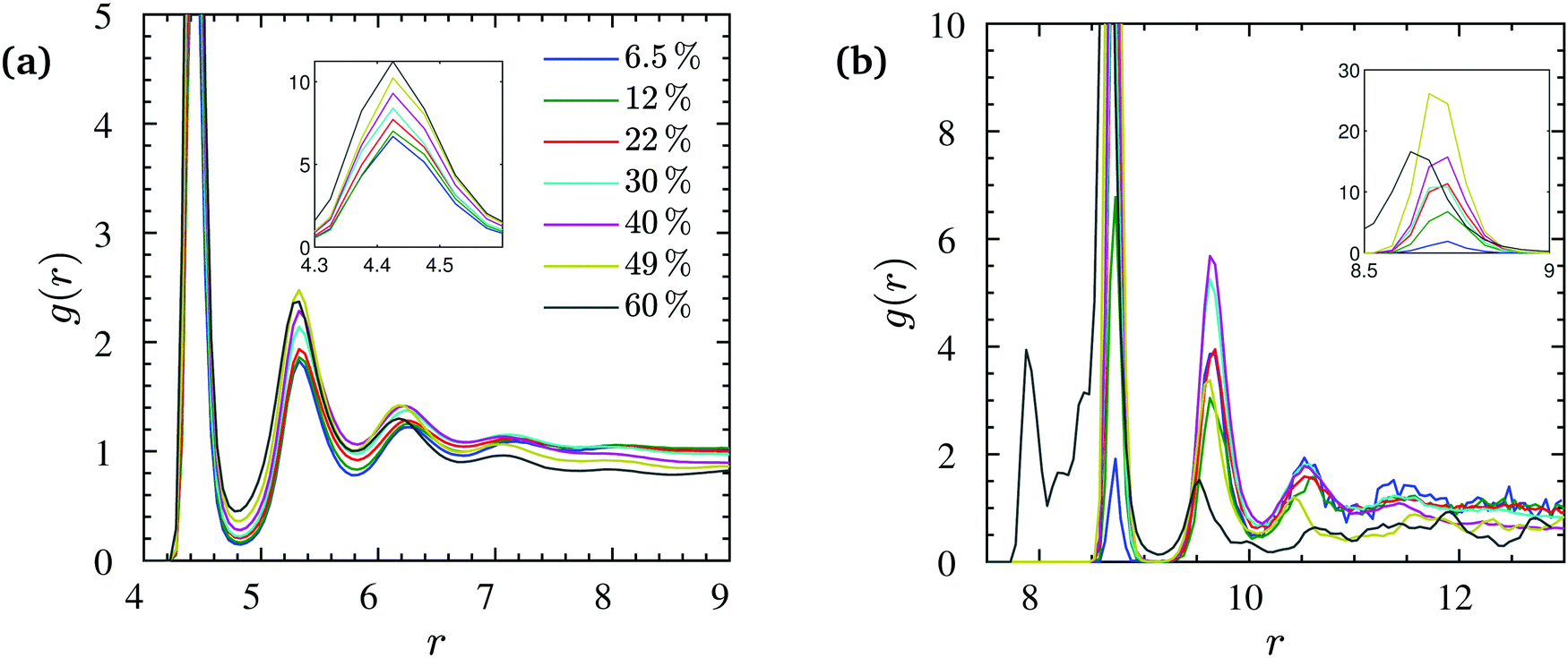 | ||
| Fig. 2 (a) NP center–monomer and (b) NP center–NP center radial distribution functions g(r) at different NP volume fractions (N = 200). The insets show the corresponding values of the first peaks in g(r) (or the second peak for ϕ = 60% in (b)). | ||
The coherent static structure factor of the polymeric subsystem, experimentally accessible via neutron scattering, is defined by
 | (3) |
 | (4) |
 | ||
| Fig. 3 (a) Static structure factor, and (b) single chain static structure factor measured at different NP volume fractions for the systems containing chains of N = 200 beads each. Dash-dotted line in (b) indicates the Debye scattering function. The inset shows inverse form factor Ssc−1 as a function of q2 at small qRg ≪ 1 for N = 200 (data for N = 100 shown in Fig. S3, ESI†). From the initial slope the radius of gyration is determined to be the same with the value of Rg = 7.4 ± 0.1 for all NP volume fractions. (c) Kratky plots corresponding to (b). The dash-dotted line shows the Kratky-representation of the Debye function as x2Ssc(x)/N = 2[exp(−x2) + x2 − 1]/x2 with x = qRg. The vertical dashed line marks the corresponding q where qRNP = 1. | ||
Furthermore, the mean squared radius of gyration Rg2 of molecules, the average squared distance between monomers and the center of mass of their molecules in a given conformation is defined as98,111
 | (5) |
 is the instantaneous center of the mass of chain α. We show in Fig. 4 that, within the error margin, the overall polymer radius of gyration of N = 100 or N = 200 remain unperturbed up to a very high load (ϕ = 60%), which denotes a very strongly confined region. The simulation predictions are in agreement with different experimental efforts in attractive nanocomposites, such as for PMMA/nanosilica mixtures by Jouault et al.17 up to ϕ ≈ 30% loading. The same unperturbed behavior is observed not only in attractive PEO/nanosilica mixtures,72 up to ϕ ≈ 53%, but also in an athermal PS/nanosilica mixtures, up to ϕ ≈ 32% loading.60
 | ||
| Fig. 4 Radius of gyration Rgversus NP volume fraction ϕ, obtained from the bead coordinates. Dash-dotted line is guide to the eyes. | ||
We use the single chain static structure factor within the qRg ≪ 1 regime as an alternative way to calculate the Rg, as it behaves as follows, Ssc(x) = N[1 − x2/3 + O(x4)] with the dimensionless x = qRg. Therefore, the radius of gyration can be evaluated from the following relation114NSsc−1(q) ≈1 + q2Rg2/3 at qRg ≪ 1 as calculated from the initial slope in the inset of Fig. 3b for N = 200 chains. The same value of Rg = 7.4 ± 0.1 was obtained from the form factor for all NP loadings, which is in perfect agreement with the direct measurements of Fig. 4 within the statistical error bars. This behavior also remained the same for N = 100 chains; see Fig. S3 (ESI†) for the single chain static structure factor and the unperturbed Rg for different NP loadings. This alternative approach further validates the observation that the Rg remains unperturbed over the relatively large NP loading range studied here. We investigated as well the tensors of gyration of all individual chains, their eigenvalues and invariants, and extracted various shape parameters. We find that there is no significant aspherity, and thus no deviation from random walk behavior, so that the radius of gyration already captures the conformational aspects (Fig. S4, ESI†).
In the following three sections we calculate, first, the degree of confinement of chains in the nanocomposite, then the polymer and NP dynamics, and finally their entanglements and corresponding effective tube diameter for different NP volume fractions and polymerization degrees.
3.2 Interparticle distance and pore size
The chains in a nanocomposite experience a geometrical confinement effect imposed by the presence of the NPs. The degree of confinement is often estimated by a mean (surface–surface) interparticle (ID) distance between NPs, assuming homogeneous distribution of NPs, as74,123 | (6) |
 | ||
| Fig. 5 Pore size definition. At a given point (red dot) that can potentially be reached by polymers, the pore radius is defined as the radius of the largest sphere (containing that point), which can be placed without any overlap with the NPs. The diameter of this particular sphere is marked by the red line. The pore size histogram is sampled by visiting all allowed points with equal probability (algorithmic details provided in Section S4, ESI†). | ||
 | ||
Fig. 6 Data for N = 200. Pore size distribution p(rp) at different NP volume fractions ϕ mentioned in the legend, normalized such that  . Similar distribution plots for N = 100 chains are presented in the Fig. S5 (ESI†). . Similar distribution plots for N = 100 chains are presented in the Fig. S5 (ESI†). | ||
The ratio dgeo/2Rg denotes the degree of confinement that polymers experience from NPs. It is depicted for N = 100 and N = 200 chains in the inset of Fig. 7 for different NP loadings. For both chain lengths studied here, it holds that dgeo/2Rg < 1, hence, they are in a strong geometrical confined regime, and the confinement ratio decreases with increasing NP loading.
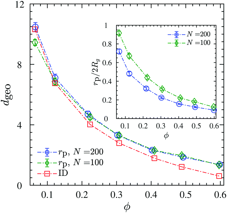 | ||
| Fig. 7 Average confinement length dgeo. Mean pore size (rp), and interparticle distance (ID) between NPs with the assumption of random dense packing as a function of NP volume fraction. The inset shows the confinement ratio dgeo/2Rg (identifying dgeo = rp) as a function of NP volume fraction. Dash-dotted lines are guides to the eye. | ||
3.3 Polymer dynamics
In this section we focus our attention on polymer rotational- and translational dynamics and its spatial modulation in the neighborhood of NPs. To calculate the chain's orientational relaxation time, we measured the autocorrelation function Cee(t) of the chain end-to-end vector Ree = rN − r1 defined by | (7) |
| Cee(t) = exp[−(t/τr)β], | (8) |
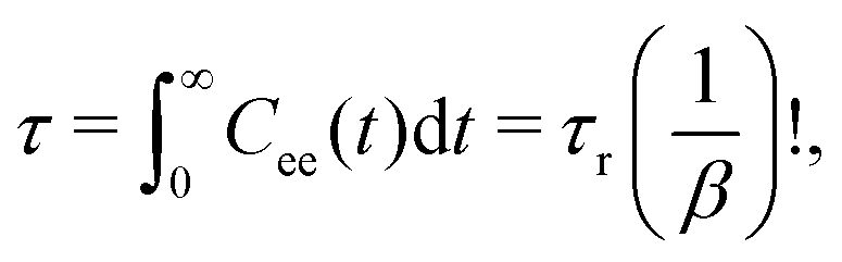 | (9) |
 | ||
| Fig. 8 (a) Chain end-to-end vector autocorrelation function Cee(t) at various NP volume fractions for N = 200. In every case Cee(0) = 1. (b) Average chain end-to-end relaxation time τ obtained from fitting of the stretched exponential function to the Cee(t) numerical values (corresponding stretched exponents β < 1 in Fig. S8, ESI†). Dash-dotted lines are guides to the eye. | ||
The mobility of polymers and NPs is very differently affected by the NP volume fraction. Regarding the overall translational mobility, we calculated the mean square displacement of polymers center of mass and NPs for different NP loadings. A sub-diffusive behavior is observed for both NPs and chain COMs over the entire NP volume fraction range studied here as shown in Fig. 9a likely due to the chain entanglements and NP confinements which may result in a cooperative dynamics. Such behavior has been observed not only experimentally, for NPs in a polymer matrix,129–131 but also from computer simulations, for polymers within porous132 or confined media.133 We can see in Fig. 9a that polymer and NP dynamics are similar at low NP volume fractions (ϕ = 6.5% and 12%) for N = 200. For higher NP loading, polymer dynamics is faster than NP dynamics, and the discrepancy increases with the NP volume fraction. A faster dynamics but with a similar trend was also observed for the N = 100 chains, but in that case polymer dynamics was faster than NP dynamics for any NP volume fraction, as shown in Fig. S7 (ESI†). There is a tendency for polymers to diffuse faster than NPs which gets enhanced with NP loading, not only because of their lower density relative to the NPs, but also because of the NP packing.
 | ||
| Fig. 9 (a) Mean-squared displacement (MSD) of NPs (solid lines) and polymer COMs (dash-dotted lines) at different NP volume fractions for N = 200. Both NPs and chain COMs indicate sub-diffusive behavior over the range of volume fractions studied here. (b) Short-time MSD of monomers relative to their closest NP center, measured at δt = 250 for N = 200 (solid lines) and N = 100 (dash-dotted lines) chains. MSD is measured as a function of monomer (initial) radial distance relative to its closest NP center at different NP volume fractions. | ||
We note here that at the large volume fraction regime ϕ ≥ 49% and in particular for the entangled systems with N = 200, the slow chain relaxation and even slower NP mobility point to the fact that these systems represent a “solid-like” behavior. In order to ensure the sampling of equilibrium states, we started the simulations from a clustered NP state and measured the 〈Rg〉 time series as well as the NP–NP pair correlation functions and found out that there is no drift in these quantities over the sampling period (see Fig. S9 and S10 (ESI†).
The short-time MSD of monomers is spatially dependent. It is shown as a function of radial distance from their closest NP in Fig. 9b for different NP loadings. The mobility of monomers increases according to their distance from NP centers, and reaches a plateau at distances far beyond the NPs surface (r > 9) for small volume fractions of ϕ ≤ 22%. This radial distance is comparable to the RNP + Rg/2 value where Rg/2 is a typical thickness of the polymer bound layer observed experimentally. We further observe a somewhat smaller plateau up to the distance of r ≈ 5.5 that corresponds to the second solvation shell of the monomers attracted to the NP surface. Larger radial distances to the NP surface cannot be reached for the high ϕ because it exceeds the ID and pore radius. It appears that within the volume fraction regime ϕ ≤ 22% the monomer mobility is rather insensitive to the NP volume fraction, while at higher NP loadings (ϕ > 22%) it slows down almost linearly with increasing ϕ, due to NP confinement that hinders polymer motion, as well as longer lasting monomer–NP temporary contacts formed in higher NP loadings.
3.4 Entanglements and tube diameter
In nanocomposites, polymer/NP (topological) entanglements control the mechanical response and viscosity of the nanocomposite. According to Schneider et al.,75 a mean field relation exists between three characteristic diameters: the apparent tube diameter dapp that can be measured by neutron spin echo (NSE) experiments, the geometric confinement length dgeo already introduced, and the diameter dtube of a “tube” in which polymer chain motion is constrained, imposed by the topological constraints of the neighboring polymer chains. The mean field equation75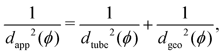 | (10) |
In our work, we calculate the primitive path networks of polymers for all NP loadings, from which we obtained the number of “kinks” Z considered to be proportional to the number of entanglements per chain, Ne = N/Z. In line with previous works,90,135 we undertook this analysis with two limits: the phantom limit, where NPs were simply ignored (Z0), and the frozen limit, where NPs served as obstacles but did not move during the minimization procedure. In the latter case we distinguish between polymer–polymer Z and polymer–NP entanglements ZNP. More specifically, in the frozen limit, not only polymers but also the NPs can give rise to kinks of the shortest disconnected path. Such kinks are located on the surfaces of the NPs and denoted as polymer–NP entanglements. All the above quantities can be seen in Fig. 10a, and in particular a strong disentanglement of chains beyond ϕ = 20% loading in the phantom limit. The decrease of entanglements with ϕ in the phantom limit is due to the diminishment of the relative amount of NP obstacles that increases with ϕ, and qualitatively similar to chain disentanglement near flat surfaces,136 that do not allow to distinguish between frozen and phantom limits. In the frozen limit however, polymer–polymer and polymer–NP entanglements increase per chain with the NP loading as the amount of obstacles provided by the NP surfaces is proportional to ϕ.
 | ||
| Fig. 10 Data for N = 200 (open symbols) and N = 100 (filled symbols). (a) Mean number of polymer–polymer Z, and polymer–NP ZNP entanglements per chain in the frozen NP limit as a function of NP volume fraction ϕ. Z0 curve shows mean number of polymer–polymer entanglements in the phantom NP limit where the NPs are simply ignored in the analysis. (b) Number density profiles of entanglements ρe(r) (frozen limit) at distance r measured from NP center at different NP volume fractions for N = 200. Dash-dotted lines are guides to the eye. | ||
The entanglement number density profile ρe(r) is shown (Fig. 10b) as a function of distance from NP centers, as well as the rheologically relevant entanglement bulk density obtained as ![[small rho, Greek, macron]](https://www.rsc.org/images/entities/i_char_e0d1.gif) e = (Z + ZNP)n/V(1 − ϕ) (Fig. S6, ESI†). An increase in entanglement number density e is found for both N = 100, 200 chains with NP loading. We determine ρe(r) using entanglements and spherical shell volumes residing within the Voronoi volume of their nearest NP. It can be seen in Fig. 10b that there is an interfacial region around NPs where the entanglement density is different from that in the bulk phase. In particular, this profile indicates two pronounced peaks within one monomer distance from the NP surface, and a minor third peak further away. The second peak (polymer–polymer entanglements) grows to the expense of the first peak (NP–polymer entanglements) with increasing ϕ while the ρe(r) for the phantom case does not exhibit such pronounced peaks. For volume fractions ϕ ≥ 22%, the magnitude of the second peak in ρe(r) exceeds the bulk value, and the NP surface seems to directly (NP contact) or indirectly (2nd layer) dominate the entanglement behavior.
e = (Z + ZNP)n/V(1 − ϕ) (Fig. S6, ESI†). An increase in entanglement number density e is found for both N = 100, 200 chains with NP loading. We determine ρe(r) using entanglements and spherical shell volumes residing within the Voronoi volume of their nearest NP. It can be seen in Fig. 10b that there is an interfacial region around NPs where the entanglement density is different from that in the bulk phase. In particular, this profile indicates two pronounced peaks within one monomer distance from the NP surface, and a minor third peak further away. The second peak (polymer–polymer entanglements) grows to the expense of the first peak (NP–polymer entanglements) with increasing ϕ while the ρe(r) for the phantom case does not exhibit such pronounced peaks. For volume fractions ϕ ≥ 22%, the magnitude of the second peak in ρe(r) exceeds the bulk value, and the NP surface seems to directly (NP contact) or indirectly (2nd layer) dominate the entanglement behavior.
We then evaluate the tube diameter dtube directly from the primitive path analysis as  with average bond length b0 = 0.97, Kuhn length bK = 1.79, and the number of entanglements Z0 per chain in the phantom NP limit.110,120,137 As depicted in Fig. 11a (with blue symbols), it is insensitive to N, because both chain lengths are located in the entangled regime, and increases with increasing ϕ.
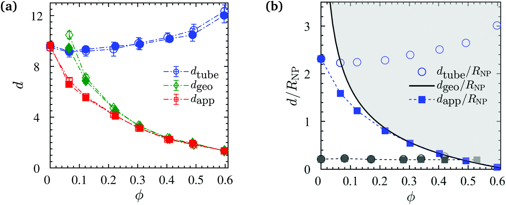 | ||
| Fig. 11 (a) Apparent tube diameter (dapp) as described in eqn (10), tube diameter from primitive path analysis (dtube) in the phantom NP limit, and average confinement length from pore size analysis (dgeo) as a function of NP volume fraction. Tube diameters at ϕ = 0 are obtained from analytical fast-converging estimators.134 (b) A comparison between different ratios of d/RNP from the current study (blue symbols) for N = 200 chains and the experimental values (gray symbols) reported by Senses et al.72 for PEO/nanosilica composites (dtube of PEO was calculated using eqn (10)). The solid black line shows the analytical formula of ID/RNP obtained from eqn (6). The shaded gray area marks the region unattainable to the apparent tube diameter dapp (filled symbols). Dash-dotted lines are guides to the eye. | ||
Upon making use of dgeo we calculate dapp from dtubeviaeqn (10). It can be seen in Fig. 11a that the apparent tube diameter decreases abruptly with the NP volume fraction up to ϕ = 20%. Such behavior was also observed in experimental measurements in PEO/nanosilica composites.72 However, this behavior was different to that observed in nanocomposites containing nonattractive interaction between polymers and NPs,75 where dapp remained constant up to ϕ = 20%. Beyond that volume fraction, dgeo coincided with dapp (red and green lines coincide for ϕ > 30%) as depicted in Fig. 11a, denoting that the term dgeo−2 ≫ dtube−2, and thus the value of dapp depend on geometric confinement (dgeo), and the disentanglement of chains originated from the random packing of NPs and the confinement they created.50 Since the radius of gyration is unperturbed by NP loading, it does not promote the disentanglement that was observed in previous studies.90,100 Moreover, the disentanglement of chains is smaller than that observed in nanocomposites with nonattractive interactions, due to the lack of expansion of the polymer radius of gyration. Again, this behavior is different from that seen in nanocomposites with nonattractive interactions,75 where dapp and dgeo coincide only at a very high NP volume fraction (ϕ > 50%).75
In recent quasielastic neutron scattering measurement (QENS) experiments in attractive nanocomposites, dapp has been measured by Senses et al.72 It is worth noting that in their study Rg (7 nm) ≪ RNP (25 nm), we thus cannot directly compare with their results as Rg ≈ 2RNP in the present work. At a given NP volume fraction their ID is 8 times larger than our ID, relative to the size of the polymers. In experiments by Senses et al.72dgeo−2 ≈ dtube−2, the geometric confinement was much weaker compared with our present simulations (ID of experiments was much larger than the ID of our simulations, thus had a larger dgeo), since large nanosilicas of 50 nm diameter were used. This led to a different trend that observed in experimental dapp (dapp remained constant for ϕ ≥ 30%).72 Senses et al.72 used ID/2Rg < 1 as a necessary and sufficient condition for dapp to be unaffected by ϕ.
Based on the mean field equation, we have thus demonstrated that this condition does not hold. To support this further, we normalized the diameters dapp, dtube (for both experiments and simulations) and ID (dgeo) with RNP, for all volume fractions, and depict these normalized ratios in Fig. 11b. It can be seen that the trend of Senses et al.72 data is much more subtle than our simulation data, due to the smaller dtube/RNP ratio. The dgeo/RNP line defines the boundary region, if approached, dapp follows dgeo. The dapp of Senses apparently just reaches the dgeo/RNP line at the highest realized NP loadings. A subsequent decrease of dapp could thus not be confirmed experimentally with the NP volume fractions that were available for their investigation.72
4 Conclusions
There is still opposing experimental (and also simulation) evidence concerning entangled polymer structure and dynamics in nanocomposites. That is especially true for the technologically relevant regime of large NP volume fractions. Thus, we investigated polymer conformations, entanglements and dynamics in attractive polymer nanocomposites, up to approximately ϕ = 60% loading, using a coarse-grained model for NPs and polymers, by means of molecular dynamics simulations. We observe an unperturbed behavior of entangled polymer chains, for the first time using simulations (polymers exhibit ideal chain statistics for 1.27 < Rg/RNP < 1.8), even at such high NP loading, in agreement with SANS experiments of attractive nanocomposites. At relatively high NP loading (ϕ ≥ 30%), chains disentangle due to geometric confinement, however, chain disentanglement was not as abrupt as in nanocomposites with nonattractive interactions. In addition, we showed based on a mean field equation, that the behavior of dapp originates from the geometrical confinement length dgeo (for ϕ ≥ 30%) and not from the dynamics of the bound polymer layer between NPs. The effect of NP volume fraction on the dapp for nanocomposites that are not studied here, with a smaller or larger ratio between tube diameter and NP size, we expect to follow the trend observed here, and apparently supported by experiment: a moderate increase of dtube with ϕ up to some critical ϕ, in the neighborhood of the NP volume fraction where dapp and dgeo meet. In order to explore smaller ratios of dtube/RNP, it would require simulating either stiffer polymers (where dtube would be smaller) or nanocomposites with larger NPs (which would require larger system sizes). Entangled polymer dynamics is reduced close to the NP surface, due to the attractive interaction, and is hindered dramatically, at high NP loadings, due to confinement.Conflicts of interest
There are no conflicts to declare.Acknowledgements
This project was supported by the Swiss National Science Foundation (grant 200021L-185052) and the Fonds National de la Recherche (FNR project INTER/SNF/18/13289828). The authors thank the Swiss National Supercomputing Centre for providing computing resources (project s987).Notes and references
- S. K. Kumar and R. Krishnamoorti, Annu. Rev. Chem. Biomol. Eng., 2010, 1, 37–58 Search PubMed.
- D. Kozuch, W. Zhang and S. Milner, Polymers, 2016, 8, 241 Search PubMed.
- A. Maiti, Microelectron. J., 2008, 39, 208–221 Search PubMed.
- S. Cheng, B. Carroll, V. Borachova, J. M. Carrillo, B. Sumpter and A. P. Sokolov, J. Chem. Phys., 2017, 146, 203201 Search PubMed.
- Y. Tien and K. Wei, Polymer, 2001, 42, 3213–3221 Search PubMed.
- K. Heo, C. Miesch, T. Emrick and R. C. Hayward, Nano Lett., 2013, 13, 5297–5302 Search PubMed.
- T. Glomann, A. Hamm, J. Allgaier, E. G. Hubner, A. Radulescu, B. Farago and G. J. Schneider, Soft Matter, 2013, 9, 10559 Search PubMed.
- L. Guadagno, L. Vertuccio, C. Naddeo, E. Calabrese, G. Barra, M. Raimondo, A. Sorrentino, W. Binder, P. Michael and S. Rana, Composites, Part B, 2019, 157, 1–13 Search PubMed.
- A. P. Holt, V. Bocharova, S. Cheng, M. Kisliuk, B. T. White, T. Saito, D. Uhrig, J. P. Mahalik, R. Kumar, A. E. Imel, T. Etampawala, H. Martin, N. Sikes, B. G. Sumpter, M. D. Dadmun and A. P. Sokolov, ACS Nano, 2016, 10, 6843 Search PubMed.
- D. N. Voylov, A. P. Holt, B. Doughty, V. Bocharova, H. M. Meyer, S. Cheng, H. Martin, M. D. Dadmun, A. Kisliuk and A. P. Sokolov, ACS Macro Lett., 2017, 6, 68–72 Search PubMed.
- V. Bocharova, A.-C. Genix, J.-M. Y. Carrillo, R. Kumar, B. Carroll, A. Erwin, D. Voylov, A. Kisliuk, Y. Wang, B. G. Sumpter and A. P. Sokolov, ACS Appl. Nano Mater., 2020, 3, 3427–3438 Search PubMed.
- P. J. Griffin, V. Bocharova, L. R. Middleton, R. J. Composto, N. Clarke, K. S. Schweizer and K. I. Winey, ACS Macro Lett., 2016, 5, 1141–1145 Search PubMed.
- I. Popov, B. Carroll, V. Bocharova, A.-C. Genix, S. Cheng, A. Khamzin, A. Kisliuk and A. P. Sokolov, Macromolecules, 2020, 53, 4126–4135 Search PubMed.
- N. Jouault, F. Dalmas, S. Said, R. Schweins, J. Jestin and F. Boue, Macromolecules, 2010, 43, 9881–9891 Search PubMed.
- A. S. Blivi, F. Benhui, J. Bai, D. Kondo and F. Bédoui, Polym. Test., 2016, 56, 337–343 Search PubMed.
- C. C. Lin, S. Gam, J. S. Meth, N. Clarke and K. I. Winey, Macromolecules, 2013, 46, 4502–4509 Search PubMed.
- N. Jouault, M. K. Crawford, C. Chi, R. J. Smalley, B. Wood, J. Jestin, Y. B. Melnichenko, L. He, W. E. Guise and S. K. Kumar, ACS Macro Lett., 2016, 5, 523–527 Search PubMed.
- W. You, W. Cui and W. Yu, Polymer, 2021, 213, 123323 Search PubMed.
- W. Cui, W. You and W. Yu, Macromolecules, 2021, 54, 824–834 Search PubMed.
- A. Papon, H. Montes, F. Lequeux, J. Oberdisse, K. Saalwächter and L. Guy, Soft Matter, 2012, 8, 4090–4096 Search PubMed.
- L. Ma, D. Zhao and J. Zheng, J. Appl. Polym. Sci., 2020, 137, 48633 Search PubMed.
- D. Zhao, G. Zhu, Y. Ding and J. Zheng, Polymers, 2018, 10, 716 Search PubMed.
- J. M. Kropka, V. G. Sakai and P. F. Green, Nano Lett., 2008, 8, 1061–1065 Search PubMed.
- Q. Jiang, Q. Zhang, X. Wu, L. Wu and J.-H. Lin, Nanomaterials, 2020, 10, 1158 Search PubMed.
- J. Odent, J.-M. Raquez, C. Samuel, S. Barrau, A. Enotiadis, P. Dubois and E. P. Giannelis, Macromolecules, 2017, 50, 2896 Search PubMed.
- J. Odent, J.-M. Raquez, P. Dubois and E. P. Giannelis, J. Mater. Chem. A, 2017, 5, 13357–13363 Search PubMed.
- J. E. Potaufeux, J. Odent, D. Notta-Cuvier, R. Delille, S. Barrau, E. P. Giannelis, F. Lauro and J.-M. Raquez, Compos. Sci. Technol., 2020, 191, 108075 Search PubMed.
- N. J. Fernandes, T. J. Wallin, R. A. Vaia, H. Koerner and E. P. Giannelis, Chem. Mater., 2014, 26, 84–96 Search PubMed.
- N. J. Fernandes, J. Akbarzadeh, H. Peterlik and E. P. Giannelis, ACS Nano, 2013, 7, 1265–1271 Search PubMed.
- K. Z. Donato, L. Matějka, R. S. Mauler and R. K. Donato, Colloids Interfaces, 2017, 1, 5 Search PubMed.
- A. Moghimikheirabadi, C. Mugemana, M. Kröger and A. V. Karatrantos, Polymers, 2020, 12, 2591 Search PubMed.
- A. Karatrantos, Y. Koutsawa, P. Dubois, N. Clarke and M. Kröger, Polymers, 2018, 10, 1010 Search PubMed.
- K. Nusser, S. Neueder, G. J. Schneider, M. Meyer, W. Pyckhout-Hintzen, L. Willner, A. Radulescu and D. Richter, Macromolecules, 2010, 43, 9837–9847 Search PubMed.
- R. Krishnamoorti, R. A. Vaia and E. P. Giannelis, Chem. Mater., 1996, 8, 1728–1734 Search PubMed.
- D. Shah, P. Maiti, D. D. Jiang, C. A. Batt and E. P. Giannelis, Adv. Mater., 2005, 17, 525 Search PubMed.
- K. Campbell, B. Gurun, B. G. Sumpter, Y. S. Thio and D. G. Bucknall, J. Phys. Chem. B, 2011, 115, 8989–8995 Search PubMed.
- F. B. Wyart and P. G. de Gennes, Eur. Phys. J. E: Soft Matter Biol. Phys., 2000, 1, 93–97 Search PubMed.
- N. Li, F. Chen, C. H. Lam and O. K. C. Tsui, Macromolecules, 2013, 46, 7889–7893 Search PubMed.
- J. T. Kalathi, G. S. Grest and S. K. Kumar, Phys. Rev. Lett., 2012, 109, 198301 Search PubMed.
- K. Nusser, G. I. Schneider, W. Pyckhout-Hintzen and D. Richter, Macromolecules, 2011, 44, 7820–7830 Search PubMed.
- D. Pimer, M. Dulle and S. Forster, Polymer, 2018, 145, 101–107 Search PubMed.
- U. Yamamoto, J.-M. Y. Carrillo, V. Bocharova, A. P. Sokolov, B. G. Sumpter and K. S. Schweizer, Macromolecules, 2018, 51, 2258–2267 Search PubMed.
- U. Yamamoto and K. S. Schweizer, Macromolecules, 2015, 48, 152 Search PubMed.
- K. Nusser, G. J. Schneider and D. Richter, Macromolecules, 2013, 46, 6263 Search PubMed.
- M. Kröger, C. Luap and R. Muller, Macromolecules, 1997, 30, 526–539 Search PubMed.
- P. S. Stephanou, J. Chem. Phys., 2015, 142, 064901 Search PubMed.
- Y.-R. Huang, Y. Jiang, J. L. Hor, R. Gupta, L. Zhang, K. J. Stebe, G. Feng, K. T. Turner and D. Lee, Nanoscale, 2015, 7, 798–805 Search PubMed.
- N. Manohar, K. J. Stebe and D. Lee, ACS Macro Lett., 2017, 6, 1104–1108 Search PubMed.
- E. J. Bailey and K. I. Winey, Prog. Polym. Sci., 2020, 105, 101242 Search PubMed.
- G. J. Schneider, K. Nusser, L. Willner, P. Falus and D. Richter, Curr. Opin. Chem. Eng., 2017, 16, 65–77 Search PubMed.
- A. Karatrantos, R. J. Composto, K. I. Winey and N. Clarke, J. Chem. Phys., 2017, 146, 203331 Search PubMed.
- A. Karatrantos, R. J. Composto, K. I. Winey and N. Clarke, Macromolecules, 2019, 52, 2513–2520 Search PubMed.
- C. C. Lin, E. Parrish and R. J. Composto, Macromolecules, 2016, 49, 5755–5772 Search PubMed.
- A. Karatrantos, N. Clarke and M. Kröger, Polym. Rev., 2016, 56, 385–428 Search PubMed.
- A. Tuteja, P. M. Duxbury and M. E. Mackay, Phys. Rev. Lett., 2008, 100, 077801 Search PubMed.
- A. I. Nakatani, W. Chen, R. G. Schmidt, G. V. Gordon and C. C. Han, Polymer, 2001, 42, 3713 Search PubMed.
- A. Nakatani, W. Chen, R. Schmidt, G. Gordon and C. Han, Int. J. Thermophys., 2002, 23, 199–209 Search PubMed.
- W. S. Tung, V. Bird, R. J. Composto, N. Clarke and K. I. Winey, Macromolecules, 2013, 46, 5345–5354 Search PubMed.
- N. Jouault, S. K. Kumar, R. J. Smalley, C. Chi, R. Moneta, B. Wood, H. Salerno, Y. B. Melnichenko, L. He, W. E. Guise, B. Hammouda and M. K. Crawford, Macromolecules, 2018, 51, 5278–5293 Search PubMed.
- M. K. Crawford, R. J. Smalley, G. Cohen, B. Hogan, B. Wood, S. K. Kumar, Y. B. Melnichenko, L. He, W. Guise and B. Hammouda, Phys. Rev. Lett., 2013, 110, 196001 Search PubMed.
- A. S. Robbes, F. Cousin, F. Meneau and J. Jestin, Macromolecules, 2018, 51, 2216–2226 Search PubMed.
- A. Banc, A.-C. Genix, C. Dupas, M. Sztucki, R. Schweins, M.-S. Appavou and J. Oberdisse, Macromolecules, 2015, 48, 6596–6605 Search PubMed.
- A.-C. Genix, M. Tatou, A. Imaz, J. Forcada, R. Schweins, I. Grillo and J. Oberdisse, Macromolecules, 2012, 45, 1663–1675 Search PubMed.
- M. Rizk, M. Krutyeva, N. Lühmann, J. Allgaier, A. Radulescu, W. Pyckhout-Hintzen, A. Wischnewski and D. Richter, Macromolecules, 2017, 50, 4733–4741 Search PubMed.
- S. Westermann, M. Kreitschmann, W. Pyckhout-Hintzen, D. Richter, E. Straube, B. Farago and G. Goerigk, Macromolecules, 1999, 32, 5793–5802 Search PubMed.
- A. L. Frischknecht, E. S. McGarrity and M. E. Mackay, J. Chem. Phys., 2010, 132, 204901 Search PubMed.
- M. Vacatello, Macromolecules, 2002, 35, 8191–8193 Search PubMed.
- F. M. Erguney, H. Lin and W. L. Mattice, Polymer, 2006, 47, 3689 Search PubMed.
- S. Chen, E. Olson, S. Jiang and X. Yong, Nanoscale, 2020, 12, 14560–14572 Search PubMed.
- S. Sen, Y. Xie, S. K. Kumar, H. Yang, A. Bansal, D. L. Ho, L. Hall, J. B. Hooper and K. S. Schweizer, Phys. Rev. Lett., 2007, 98, 128302 Search PubMed.
- Y. Golitsyn, G. J. Schneider and K. Saalwachter, J. Chem. Phys., 2017, 146, 203303 Search PubMed.
- E. Senses, S. Darvishi, M. S. Tyagi and A. Faraone, Macromolecules, 2020, 53, 4982–4989 Search PubMed.
- S. Gam, J. S. Meth, S. G. Zane, C. Chi, B. A. Wood, M. E. Seitz, K. I. Winey, N. Clarke and R. J. Composto, Macromolecules, 2011, 44, 3494 Search PubMed.
- S. Gam, J. S. Meth, S. G. Zane, C. Chi, B. A. Wood, K. I. Winey, N. Clarke and R. J. Composto, Soft Matter, 2012, 8, 6512 Search PubMed.
- G. J. Schneider, K. Nusser, L. Willner, P. Falus and D. Richter, Macromolecules, 2011, 44, 5857–5860 Search PubMed.
- E. J. Bailey, P. J. Griffin, R. J. Composto and K. I. Winey, Macromolecules, 2020, 53, 2744–2753 Search PubMed.
- E. J. Bailey, P. J. Griffin, M. Tyagi and K. I. Winey, Macromolecules, 2019, 52, 669–678 Search PubMed.
- N. Jouault, J. F. Moll, D. Meng, K. Windsor, S. Ramcharan, C. Kearney and S. K. Kumar, ACS Macro Lett., 2013, 2, 371–374 Search PubMed.
- T. V. M. Ndoro, E. Voyiatzis, A. Ghanbari, D. N. Theodorou, M. C. Bohm and F. Müller-Plathe, Macromolecules, 2011, 44, 2316–2327 Search PubMed.
- I. G. Mathioudakis, G. G. Voyiatzis, E. Voyiatzis and D. N. Theodorou, Soft Matter, 2016, 12, 7585–7605 Search PubMed.
- D. Brown, P. Mele, S. Marceau and N. D. Alberola, Macromolecules, 2003, 36, 1395 Search PubMed.
- H. Emamy, S. K. Kumar and F. W. Starr, Macromolecules, 2020, 53, 7845–7850 Search PubMed.
- F. W. Starr, T. B. Schröder and S. C. Glotzer, Phys. Rev. E: Stat., Nonlinear, Soft Matter Phys., 2001, 64, 021802 Search PubMed.
- A. Karatrantos, R. J. Composto, K. I. Winey and N. Clarke, Macromolecules, 2011, 44, 9830–9838 Search PubMed.
- Q.-H. Yang, C.-J. Qian, H. Li and M.-B. Luo, Phys. Chem. Chem. Phys., 2014, 16, 23292–23300 Search PubMed.
- T. Desai, P. Keblinski and S. K. Kumar, J. Chem. Phys., 2005, 122, 134910 Search PubMed.
- M. Goswami and B. G. Sumpter, J. Chem. Phys., 2009, 130, 134910 Search PubMed.
- P. J. Dionne, R. Osizik and C. R. Picu, Macromolecules, 2005, 38, 9351–9358 Search PubMed.
- T. Chen, H. J. Qian, Y. L. Zhu and Z. Y. Lu, Macromolecules, 2015, 48, 2751–2760 Search PubMed.
- A. Karatrantos, N. Clarke, R. J. Composto and K. I. Winey, Soft Matter, 2016, 12, 2567 Search PubMed.
- Y. Termonia, Polymer, 2009, 50, 1062–1066 Search PubMed.
- M. S. Ozmusul, C. R. Picu, S. S. Sternstein and S. K. Kumar, Macromolecules, 2005, 38, 4495 Search PubMed.
- M. Vacatello, Macromolecules, 2001, 34, 1946–1952 Search PubMed.
- Q. W. Yuan, A. Kloczkowski, J. E. Mark and M. A. Sharaf, J. Polym. Sci., Polym. Phys. Ed., 1996, 34, 1647–1657 Search PubMed.
- G. G. Vogiatzis, E. Voyiatzis and D. N. Theodorou, Eur. Polym. J., 2011, 47, 699–712 Search PubMed.
- M. A. Sharaf and J. E. Mark, Polymer, 2004, 45, 3943–3952 Search PubMed.
- E. Y. Lin, A. L. Frischknecht and R. A. Riggleman, Macromolecules, 2020, 53, 2976–2982 Search PubMed.
- A. Karatrantos, N. Clarke, R. J. Composto and K. I. Winey, Soft Matter, 2015, 11, 382 Search PubMed.
- A. Karatrantos, N. Clarke, R. J. Composto and K. I. Winey, IOP Conf. Ser.: Mater. Sci. Eng., 2014, 64, 012041 Search PubMed.
- Y. Li, M. Kröger and W. K. Liu, Phys. Rev. Lett., 2012, 109, 118001 Search PubMed.
- J. Liu, Y. Wu, J. Shen, Y. Gao, L. Zhang and D. Cao, Phys. Chem. Chem. Phys., 2011, 13, 13058–13069 Search PubMed.
- A. Karatrantos, R. J. Composto, K. I. Winey, M. Kröger and N. Clarke, Macromolecules, 2012, 45, 7274 Search PubMed.
- H. Eslami, M. Rahimi and F. Müller-Plathe, Macromolecules, 2013, 46, 8680–8692 Search PubMed.
- X.-M. Jia, H.-J. Qian and Z.-Y. Lu, Phys. Chem. Chem. Phys., 2020, 22, 11400–11408 Search PubMed.
- Y. Song and Q. Zheng, Crit. Rev. Solid State Mater. Sci., 2016, 41, 318–346 Search PubMed.
- G. Allegra, G. Raos and M. Vacatello, Prog. Polym. Sci., 2008, 33, 683–731 Search PubMed.
- M. Wang, K. Zhang, D. Hou and P. Wang, Nanoscale, 2020, 12, 24107–24118 Search PubMed.
- S. Sen, Y. Xie, A. Bansal, H. Yang, K. Cho, L. S. Schadler and S. K. Kumar, Eur. Phys. J.: Spec. Top., 2007, 141, 161 Search PubMed.
- K. Kremer and G. S. Grest, J. Chem. Phys., 1990, 92, 5057 Search PubMed.
- M. Kröger and S. Hess, Phys. Rev. Lett., 2000, 85, 1128–1131 Search PubMed.
- M. Rubinstein and R. H. Colby, Polymer Physics, Oxford University Press Inc., New York, 2003 Search PubMed.
- K. Hagita, T. Murashima and N. Iwaoka, Polymers, 2018, 10, 1224 Search PubMed.
- H. R. Warner, Ind. Eng. Chem. Fundam., 1972, 11, 379–387 Search PubMed.
- M. Kröger, W. Loose and S. Hess, J. Rheol., 1993, 37, 1057–1079 Search PubMed.
- T. Deguchi and E. Uehara, Polymers, 2017, 9, 252 Search PubMed.
- M. Kröger, J. Non-Newtonian Fluid Mech., 2015, 223, 77–87 Search PubMed.
- A. Moghimikheirabadi, L. M. C. Sagis, M. Kröger and P. Ilg, Phys. Chem. Chem. Phys., 2019, 21, 2295–2306 Search PubMed.
- M. P. Allen and D. J. Tildesley, Computer Simulation of Liquids, Clarendon Press, Oxford, UK, 1987 Search PubMed.
- J. X. Hou, C. Svaneborg, R. Everaers and G. S. Grest, Phys. Rev. Lett., 2010, 105, 068301 Search PubMed.
- R. S. Hoy, K. Foteinopoulou and M. Kröger, Phys. Rev. E: Stat., Nonlinear, Soft Matter Phys., 2009, 80, 031803 Search PubMed.
- A. Moghimikheirabadi, L. M. Sagis and P. Ilg, Phys. Chem. Chem. Phys., 2018, 20, 16238–16246 Search PubMed.
- S. Plimpton, J. Comp. Physiol., 1995, 117, 1–19 Search PubMed.
- S. Wu, Polymer, 1985, 26, 1855–1863 Search PubMed.
- Y. Akiyama, H. Shikagawa, N. Kanayama, T. Takarada and M. Maeda, Small, 2015, 11, 3153–3161 Search PubMed.
- Y. T. Park, Y. Qian, C. I. Lindsay, C. Nijs, R. E. Camargo, A. Stein and C. W. Macosko, ACS Appl. Mater. Interfaces, 2013, 5, 3054–3062 Search PubMed.
- B. L. Frankamp, A. K. Boal and V. M. Rotello, J. Am. Chem. Soc., 2002, 124, 15146–15147 Search PubMed.
- Z. Zhang, Z. Feng, R. Tian, K. Li, Y. Lin, C. Lu, S. Wang and X. Xue, Anal. Chem., 2020, 92, 7794–7799 Search PubMed.
- A. Kutvonen, G. Rossi and T. Ala-Nissila, Phys. Rev. E: Stat., Nonlinear, Soft Matter Phys., 2012, 85, 041803 Search PubMed.
- M. Lungova, M. Krutyeva, W. Pyckhout-Hintzen, A. Wischnewski, M. Monkenbusch, J. Allgaier, M. Ohl, M. Sharp and D. Richter, Phys. Rev. Lett., 2016, 117, 147803 Search PubMed.
- G. S. Schneider, K. Nusser, S. Neueder, M. Brodeck, L. Willner, B. Farago, O. Holderer, W. J. Briels and D. Richter, Soft Matter, 2013, 9, 4336–4348 Search PubMed.
- E. Senses, S. Narayanan and A. Faraone, ACS Macro Lett., 2019, 8, 558–562 Search PubMed.
- G. M. Foo, R. B. Pandey and D. Stauffer, Phys. Rev. E: Stat., Nonlinear, Soft Matter Phys., 1996, 53, 3717 Search PubMed.
- P. Polanowski and A. Sikorski, J. Mol. Model., 2019, 25, 84 Search PubMed.
- R. S. Hoy, K. Foteinopoulou and M. Kröger, Phys. Rev. E: Stat., Nonlinear, Soft Matter Phys., 2009, 80, 031803 Search PubMed.
- G. N. Toepperwein, N. C. Karayiannis, R. A. Riggleman, M. Kröger and J. J. de Pablo, Macromolecules, 2011, 44, 1034 Search PubMed.
- G. Giunta, C. Svaneborg, H. A. Karimi-Varzaneh and P. Carbone, ACS Appl. Polym. Mater., 2020, 2, 317–325 Search PubMed.
- R. S. Hoy and M. Kröger, Phys. Rev. Lett., 2020, 124, 147801 Search PubMed.
Footnote |
| † Electronic supplementary information (ESI) available: NP–NP radial distribution function, single chain structure factor, pore size distribution, and MSD graphs for N = 100 chains; single chain structure factor in the intermediate qRg regime for N = 200 chains; gyration tensor analysis, stretched exponents, and entanglement number densities for both N = 100, 200 chains. See DOI: 10.1039/d1sm00683e |
| This journal is © The Royal Society of Chemistry 2021 |