Design of vesicle prototissues as a model for cellular tissues

Abstract

Synthesizing biomimetic prototissues with predictable physical properties is a promising tool for the study of cellular tissues, as they would enable to test systematically the role of individual physical mechanisms on complex biological processes. The aim of this study is to design a biomimetic cohesive tissue with tunable mechanical properties by the controlled assembly of giant unillamelar vesicles (GUV). GUV–GUV specific adhesion is mediated by the inclusion of the streptavidin–biotin pair, or DNA complementary strands. Using a simple assembly protocol, we are capable of synthesizing vesicle prototissues of spheroidal or sheet-like morphologies, with predictable cell–cell adhesion strengths, typical sizes, and degree of compaction.

---

1 Introduction

Nature represents an endless source of inspiration for scientists. Biomimetic approaches have been developed with the aim of reproducing particular features displayed by living organisms for targeted functions. Synthetic biology gets inspiration from biological systems, with the goal of redesigning them or even conceiving new artificial biological systems displaying specific capabilities. Such bottom-up approaches led to the fabrication of artificial cells and tissues.^1–4 This approach can be beneficial in order to develop promising biomedical or pharmaceutical applications, but also very valuable for fundamental research. The manipulation of artificial cells can be suited for the study of cell properties or cellular mechanisms, which are challenging to tackle using living cells, due to their inherent complexity or its multifactorial nature.^5–7 In this context, a diversity of simplified biomimetic artificial cells has been developed, displaying a reduced degree of complexity. Whereas these cell models can be diverse in architecture (droplets, coacervates, liposomes, polymersomes^1,8) giant unilamellar vesicles (GUVs) represent one of the most relevant biomimetic prototypes.⁹

GUVs are constituted of a phospholipid semi-permeable bilayer. The biochemical membrane composition can be enriched at will by using specific lipid mixtures and the inclusion of membrane proteins. However, GUVs are reductionist cell models since they are passive objects that cannot actively move, exchange, nor exhibit mechano-transduction mechanisms, reproduce, or die. Vesicles are soft objects with a membrane bending modulus of about tenths of k_BT, and are prone to display large membrane fluctuations due to thermal agitation. Their low lysis tension makes them susceptible to form membrane pores under moderate osmotic pressure differences between the inner and outer buffer. Over the last decades vesicles have been employed to model the biochemistry and biophysics of cells.¹ A huge effort has been done in the community in making GUVs akin to living cells, for example by reproducing lipid rafts on their membranes,⁵ taking into account additional inner compartmentalisation (with the inclusion of smaller daughter vesicles),¹⁰ or by arming the GUV membrane with an inner active shell of actin.¹¹ The goal of the present paper is not focused on the development of single cell features, but on the controlled assembly of an ensemble of vesicles for the formation of a vesicle prototissue, as a model for cellular tissues. Biological tissues are extremely complex systems. On top of the complexity of individual cells, tissues are formed from the interconnection between adjacent cells mediated by cell–cell adhesion sites enabling collective functions. Living tissues are inherently out-of-equilibrium systems. Cell-division and apoptosis are at play, as well as exchange of information between cells and the surrounding environment (through mechano-sensing systems), giving rise to a dynamic tissue reorganization. In addition, in specific biological processes, such as embryogenesis, tumor metastasis or wound healing, tissues are prone to migrate and reshape extensively over relative short time scales of minutes or hours, resulting into the occurrence of collective tissue flows.¹² Extraordinary progress on the understanding of biological mechanisms regulating living tissues has been achieved over the last decades, partly based on the development of animal models.^13–15 However, in vivo models it is extremely challenging to uncouple and elucidate the role of different underlying mechanisms. Biomimetic approaches, instead, offer the possibility to design experiments to selectively probe specific mechanisms involved in living tissues, and to get a quantitative insight.

In living cells, cell–cell adhesion is mediated by cell adhesion molecules (CAMs) present in the cell membrane bridging adjacent cells. Cell adhesion results from a combination of attractive interaction due to specific bonding of CAMs, repulsion originating from the outer cell glycocalyx, and membrane elasticity.^16,17 There is evidence of a large number of active mechanisms taking part in cell adhesion (i.e. a complex signaling network orchestrating CAMs, interaction of binding sites with cell cytoskeleton, mechano-sensing processes, etc.).¹⁸ Nonetheless, an important part of cell adhesion is due to passive physical mechanisms involving lateral diffusion of binding molecules and cell elasticity.^16,19 These mechanisms can be investigated in depth making use of biomimetic cell models. The number of attempts to develop GUV-prototissues is, up to now, limited.^20,21 Amorphous 3D vesicle aggregates have been produced using vesicle constructs adhering thanks to a ligand–receptor pair such as streptavidin–biotin^22–26 or lectin-carbohydrates,²⁷ and thanks to the specificity between complementary DNA strands,^28–31 and also by means of non-specific adhesion mediated by electrostatic interactions.^32,33 The streptavidin–biotin pair, although it displays a bonding strength of 35k_BT, well above biological bonds involved in cell–cell adhesion, has been greatly employed in mimicry studies and in biotechnological applications due to its robustness and well-characterized interaction.^34–36 Such large binding affinities makes vesicle–vesicle adhesion energetically favorable, overcoming unfavorable nonspecific interactions (Helfrich membrane fluctuations, electrostatics, or steric repulsion).¹⁶ Further developments on biomimetic prototissues have been implemented with the goal of reproducing specific tissue functions: communication between compartments, by the formation of lipid nanotubes³⁷ or the inclusion of protein pores³⁸ on the membranes connecting the interior of adjacent vesicles; external manipulation of GUVs using optical tweezers³⁸ or magnetic fields³⁹ has also offered the possibility to fabricate predictable 3D spatial arrangements; and thermoresponsive functions of vesicles (or proteinosome) prototissues have been implemented using DNA-based technologies⁴⁰ (or thermoresponsive polymers⁴¹), leading to reversible compaction of tissues.

The goal of the present work is to design a prototissue by the assembly of GUVs in the presence of ligand and receptors at suitable concentrations. Two ligand–receptor systems have been implemented: the inclusion of the biotin–streptavidin complex and the adhesion based on the complementarity of single-stranded-DNA chains. Using a simple assembly protocol for which we only adjust the mixing method, as well as vesicle and ligand and receptor concentrations, we are capable of synthesizing vesicle prototissues of spheroidal or sheet-like morphologies with predictable cell–cell adhesion strengths, typical sizes, and degree of compaction. The tissue properties can be tuned independently, which opens the possibility to isolate the role of specific physical properties and unravel their individual role in complex physiological problems.

The article is organized in the following way. Section 2 includes details on Materials and Methods. Results and discussion are presented altogether in Section 3. First, the different regimes recovered for vesicle aggregation are qualitatively displayed in a phase diagram (Section 3.1). Next, we quantify the properties of adhesive vesicles (Section 3.2). We then characterize the size of vesicle prototissues (Section 3.3) and their morphology, 3d vs. 2d-structures and cohesion (Section 3.4). Finally the conclusions of our work are drawn in Section 4.

2 Materials and methods

2.1 Vesicle fabrication

Giant unilamellar vesicles were produced by electroformation.⁴² The lipid mixture used was either Egg-PC (Sigma Aldrich, P3556) alone or Egg-PC and DSPE-PEG(2000)-Biotin (Avanti Lipids, 880129P) at molar fractions 1.25, 2.5, 5 and 10%. Fluorescence of the vesicle membrane was provided by adding either 16 : 1 Liss Rhodamine PE (Avanti Polar Lipids 810158, red marker, with λ_abs = 560 nm and λ_em = 583 nm) or NBD-PE (Avanti Polar Lipids 810141, green marker, with λ_abs = 460 nm and emission at λ_em = 535 nm) at 1% mol. The electroformation chamber was prepared by spreading 50 μL of the lipid mixture on two ITO slides (Sigma Aldrich, 636916), left under vacuum for at least 1 h 30 min to evaporate the solvent. The slides were then placed facing each other using a 1 mm thick PDMS spacer. The chamber was filled with a filtered 290 mOsm sucrose (Sigma Aldrich, S7903) solution prepared with ultrapure Milli-Q water. An alternative tension was applied between both slides at a frequency of 10 Hz, and the amplitude was gradually increased from 0.2 to 1.2 V for a total duration of 2 hours, with a final step at 4 Hz and 1 V for 30 minutes in order to enhance vesicle detachment from the slides. The electroformed vesicles were collected and stored in a plastic tube at 4 °C for a maximum of one week. In assembly experiments, vesicles were dispersed in a glucose solution at 300 mOsm. A difference in osmolarity between the outer and inner vesicle solutions was maintained constant to +10 mOsm, which enabled vesicles to slightly deflate.

In view of the assembly experiments, it was important to control the volume fraction of vesicles used in each experiment. Since the yield of vesicle production differed from one electroformation to another, we quantified the volume fraction of vesicles for each electroformation and dilute the solution in order to start assembly experiments at a concentration of reference that we set to c₀ = (3.3 ± 0.5) × 10³ vesicles per μL. In order to estimate the concentration of vesicles in the electroformed solution we used a counting procedure: 10 μL of the vesicle solution were placed in an observation chamber filled with a glucose solution (less dense than the inner sucrose solution) so that all vesicles sedimented at the bottom of the chamber (at a same focal plane). We took several images of the vesicles in phase-contrast microscopy and used an ImageJ routine in order to count the number of vesicles per unit area to extrapolate the vesicle volume fraction, and estimate the overall vesicle concentration assuming homogeneous distribution of vesicles within the chamber. A size threshold for the vesicle radius, r_min = 1 μm, was set in order to disregard impurities in the counting procedure. The computed average radius of the electroformed vesicles was r = 6 ± 3 μm (an histogram with the typical size distribution of electroformed vesicles is provided in the ESI†).

2.2 Assembly protocol

2.2.1 Assembly with streptavidin–biotin. Streptavidin (SA) is a tetrameric protein that has four binding sites for biotin. Biotinylated lipids were present on vesicle membranes, enabling bridging between adjacent vesicles. In the following, we will refer to biotinylated lipids as receptors and to SA molecules as ligands. In our experiments we used fluorescent texas Red Streptavidin Conjugate (Fisher Scientific, 10338002), enabling the visualization and quantification of vesicle–vesicle contacts by confocal microscopy. SA was stocked in PBS (292 mOsm) at a concentration of 1 mg mL⁻¹ and stored at 4 °C for one month. Necessary amounts of SA were added to the solution of biotinylated vesicles to match the X ratios. Experimentally, X was computed as the total number of SA molecules in solution (N_SA) to the total number of biotin molecules contained on the outer leaflet of vesicle membranes (N_b), according to the biotin molar ratio used in the lipid mixture for the electroformation, and taking into account the total number of vesicles present in the assembly mixture, so that X = N_SA/N_b. Since electroformed vesicles displayed an important polydispersity, we took into account the vesicle size distribution for the estimation of the mean vesicle surface. In our experiments, X values ranged from 0.4 to 40. Larger values of X could not be attained experimentally, as we observed vesicle degradation. After addition of SA, the samples were left incubating for approximately 2 h. For larger incubation times, the typical sizes of the aggregates did not increase significantly. After 24 hours of incubation, however, we observed degradation of vesicles (deflated vesicles, as well as the apparition of vesicle debris in solution).

We used three different modes of incubation: Concentration (C), Sedimentation (S), and in-plane Rotation (R), illustrated in Fig. 1. In the Concentration method, an initial volume of the electroformed-vesicles solution (ranging from 10 to 400 μL) was mixed with a volume of glucose solution (300 mOsm) 1.5 times larger, and centrifuged at 7g during 30 min. Due to the difference in density between the inner- and outer-vesicle solutions vesicles were driven to the bottom of the tube. Next, the upper supernatant solution (free of vesicles) was removed and only 10 μL were left, and then the necessary volume of SA solution was added (ranging from 0.1 to 10 μL). After an incubation period of 2 hours, the aggregate solution was gently pipetted and deposited into an observation chamber, which was then filled with glucose solution to a final volume of 100 μL. In the Sedimentation method a fixed volume of the vesicle solution (20 μL) was added to 80 μL of the glucose solution into a plastic tube. The centrifugation stage was omitted in this protocol and vesicles were driven towards the bottom part of the tube solely by the gravitational force. In the in-plane-Rotation method, 20 μL of the vesicle solution were added to 80 μL of the glucose solution directly in an observation chamber, so that the incubation step was performed in the chamber. During incubation, an in-plane rotation was applied by means of a rotating plate device at 60 rpm, in order to enhance in-plane vesicle–vesicle encounters. This method is used for cell culturing in wells, which are swirled on an orbital shaker in order to generate a flow inside the well.⁴³ Since the area of the observation chamber we used was about 3 times larger than the area occupied by the total number of vesicles in solution, vesicle assembled forming a 2D-vesicle layer. Concentration and Sedimentation protocols were favored in order to obtain 3D aggregates while the Rotating method led to the formation of 2D monolayers.

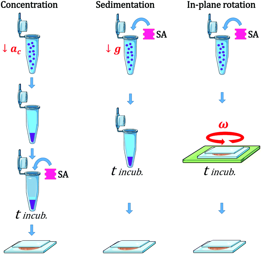Fig. 1 Scheme representing the different protocols used for the vesicle assembly: Concentration (C), Sedimentation (S), and Rotation (R). In (C) vesicle–vesicle encounters were driven by a centrifugation step (at centripetal acceleration a_c = 7 g), while in (S) they were solely driven by the gravitational force. In (R), an in-plate rotation of 60 rpm was applied. In all protocols the incubation time (t_incub) was set to 2 h.

2.2.2 Assembly with DNA complementary strands. Vesicle assembly was also achieved using complementary DNA strands. The DNA linkers consisted of a cholesterol which anchored to the vesicle membrane, followed by a spacer made of a DNA double strand with a length of 43 base pairs, and were ended with a 9 bases sequence of single stranded DNA, that acted as sticky end.⁴⁰ The interaction of a sticky end with its complementary strand was the mechanism driving the assembly of the vesicles. This interaction is mediated by hydrogen bonding between complementary base pairs (A: T, C: G). We used the same DNA sequences designed by Parolini et al.⁴⁰ (IDT Company) with a binding energy of 18.3k_BT. Equal amounts of DNA complementary constructs were added to the vesicle solution, at a total concentration of 32 or 644 nM. Fluorescence of the DNA was provided by adding 2 μM of the intercalating dye SYTO 64 (λ_abs = 599 nm, λ_em = 619 nm, Thermo Fisher). Further details on the fabrication of DNA constructs and DNA mediated assembly are provided in the ESI.†

2.3 Visualization of vesicle aggregates

For vesicle prototissue imaging, we prepared observation chambers with an Ace O-ring (Sigma Aldrich, Z504696) fixed to a glass coverslip using UV-glue (Norland), that we previously cleaned and functionalized with β-casein bovine (Sigma Aldrich, C6905).¹¹ To prevent evaporation, samples were covered with a glass coverslip and sealed with grease before proceeding to image acquisition. Phase contrast and epifluorescence images were obtained with an inverted microscope (DMIRB, Leica) with objectives ×10 (NA = 0.25) or ×20 (NA = 0.4) and a Hamamatsu camera (C13440 ORCA-flash 4.0). The source of light for fluorescence imaging was a CoolLED pE-300 white LED lamp. Confocal images were obtained with a confocal microscope (Zeiss LSM880) and with a ×40 objective (water immersion, NA = 1.1). Signal acquisition was performed with two detectors (GaAsP and PMT) used respectively for an Argon laser (λ = 488 nm), and for an He/Ne laser (λ = 633 nm).

2.4 Quantification of aggregate properties

2.4.1 Membrane fluorescence. In order to assess quantitatively the concentration of fluorescent molecules on vesicle membranes, the equatorial plane of single vesicles or vesicles forming vesicle doublets was imaged using confocal microscopy. With the ImageJ Radial profile tool, a circle (or an arch) were placed to fit a whole vesicle (or a part of its membrane) to obtain the integrated fluorescence intensity, normalized by the perimeter (or arch length), as shown schematically in the inset of Fig. 3B. Analogously, in order to perform the fluorescence quantification of the adhesion patch we fitted a rectangle at the interface between the two vesicle membranes to obtain the integrated fluorescence intensity, normalized by the length of the patch. Both routines were applied to the red and green channels corresponding to the red SA and green lipid marker incorporated into the membranes.

2.4.2 Contact angle of vesicle doublets. Vesicle–vesicle adhesion was quantified by measuring the equilibrium contact angle (θ) between two vesicles of comparable vesicle sizes,^35,44–47 that we call a vesicle doublet. Vesicle doublets were prepared by adding necessary amounts of SA to a solution of biotinylated vesicles at a vesicle volume fraction of 0.25%, and incubating them for 2 h in a tube rotator at room temperature. This high dilution protocol favored the assembly of vesicles into doublets and minimized the formation of vesicle aggregates. The samples were imaged in confocal microscopy. A z-scan of each doublet was performed in order to identify the largest length of the adhesion patch (corresponding to their equatorial plane) which was used for the quantitative analysis. We analyzed doublets formed by two vesicles of comparable sizes (with a size difference below 20%) and a flat vesicle–vesicle interface. The contact angle was obtained by fitting a circle to each vesicle, and computed after the radii of the two vesicles (R₁, R₂), and the coordinates of their centers (see ESI† for further details). A sketch is shown in the inset of Fig. 3A. The number of doublets analyzed for all conditions was set to N = 20.

2.4.3 3d-aggregate sizes. The vesicle prototissues obtained using the Concentration and Sedimentation protocols had a 3-dimensional structure. 3d-imaging and quantification of object sizes was performed by confocal microscopy. Aggregate volumes were measured using Imaris Software (Oxford Instruments) which enables 3d-reconstitution of aggregates from 2d z-stacks obtained with confocal microscopy, with a final resolution along the z-axis of 1 μm. The software enabled the determination of the overall external surface and the enclosed volume of the aggregate, but did not identify possible inner voids contained within the structure.

3 Results and discussion

3.1 Aggregation phase diagram

Vesicle aggregation was shown to depend on the concentration of ligands (SA molecules) in solution and receptors (biotin-lipids) on vesicle membranes. In the phase diagram of Fig. 2 the different aggregation states can be distinguished. For very low SA concentrations (low X), and regardless of the lipid-biotin content, vesicle aggregation did not take place. In this situation the number of receptor–ligand–receptor bridges per vesicle was too low to enable the adhesion between adjacent vesicles (control experiments performed with no SA in solution led to no vesicle aggregation).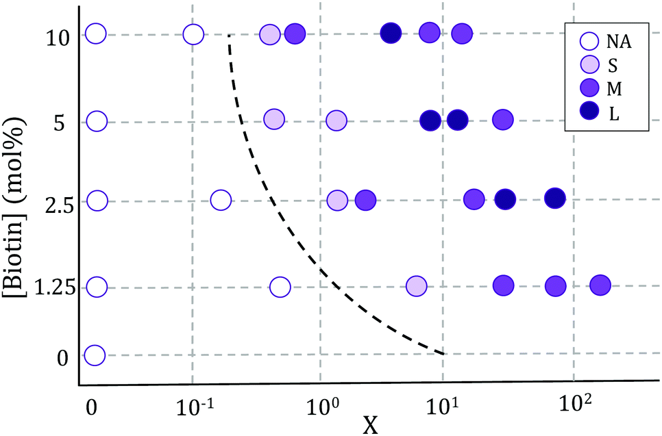

Fig. 2 Phase diagram of vesicle aggregation as a function of biotin concentration and X = N_SA/N_b, obtained using the Sedimentation (S) protocol. Maximal aggregate sizes for each condition are indicated as: S (small aggregates) <4 × 10³ μm²; 4 × 10³ μm² < M (medium-size aggregates) <2 × 10⁴ μm²; L (large aggregates) >2 × 10⁴ μm². NA stands for ‘no aggregation’.

For a given biotin-lipid content, as the SA concentration was increased, vesicle–vesicle doublets were first obtained, and assemblies of multiple vesicles in aggregates formed at larger SA concentrations. In Fig. 2, we distinguish between small (size < 4 × 10³ μm²), medium (4 × 10³ μm² < size < 2 × 10⁴ μm²) and large (size > 2 × 10⁴ μm²) aggregates, which are depicted with different color intensities (as obtained from 2D images, sizes correspond to the maximal projection on the plane; more accurate 3d-quantitative data are provided in Section 3.3). By increasing the concentration of SA, most biotin-lipids got saturated by SA, preventing further vesicle–vesicle adhesion, and limiting the size of vesicle aggregates and eventually completely inhibiting vesicle aggregation. This trend is partly visible in Fig. 2, for 5% and 10% mol biotin, for which aggregate sizes decrease for the largest X values. Thus, the vesicle aggregation process was initiated but also inhibited by free SA in solution, in agreement with previous experimental works.^23,29,48 For a constant X ratio, aggregate sizes increased with increasing biotin-lipid content, as this entailed an increasing number of available receptors and a larger potential number of bridges that could be formed between vesicles. The assembly protocol used for vesicle aggregation also played a relevant role in the aggregation phase diagram. The Concentration protocol systematically led to vesicle aggregates with typical larger sizes compared to the Sedimentation protocol, regardless of the X ratio and biotin content (not shown in the figure). We can rationalize the dynamics of vesicle assembly in terms of the time scale for vesicle–vesicle encounter (t_ves–ves). In the Sedimentation (S) protocol (used for results shown in Fig. 2) vesicle–vesicle collisions were only driven by sedimentation. Typical times for vesicle–vesicle encounters can be approximated by the sedimentation time of vesicles inside the incubation tube. Considering the Stokes regime and an incubation volume of 100 μL, this leads to t_ves–ves ≃ 15 min. Note however, that this is an overestimation as we disregard the possibility for vesicle–vesicle encounters to take place before reaching the bottom of the incubation tube. The adsorption of free SA in solution onto vesicle membranes takes place during this lapse of time before two vesicles encounter. Aggregation kinetics thus results from a combination of both vesicle–vesicle encounters and diffusion of free SA to vesicle membranes, which makes it difficult to control. Note that this competition will also be dependent on the X ratio. For large X values (X ≫ 1) vesicle surfaces may become saturated by SA before encountering another vesicle, thus hindering further vesicle bridging. In order to gain control on the assembly process, we privileged the Concentration (C) protocol for which vesicles were brought to close contact by a centrifugation stage prior to the addition of SA, greatly reducing the vesicle encounter time. Kinetics play a minor role in this protocol, which makes it more suitable for the synthesis of aggregates of controlled sizes (we will use this protocol in Section 3.3 when controlling aggregate sizes).

In all incubation methods, the incubation volume for vesicle assembly was considerably larger than the volume fraction of vesicles. Thus, it is likely that not all SA molecules could reach the biotin groups on vesicles surfaces within the incubation time of 2 h, and that a fraction of SA could remain free in solution. As a consequence, the ratio X (computed as the number of SA molecules in solution over the biotin-lipids on vesicle membranes, X = N_SA/N_b) does not necessarily coincide with the average ligand-to-receptor ratio on vesicle membranes. In the following, however, we will refer to X as the ligand-to-receptor ratio. Vesicle–vesicle bridging should be maximized for X = 0.25, corresponding to a an equal number of receptors and ligand sites (4 sites per SA molecule).⁴⁸ In practice, and due to the presence of free SA molecules in solution, we obtained the largest aggregate sizes (Fig. 2), as well as maximal contact angles for vesicle doublets (in Fig. 3A), for X > 0.25. Analogously, X ≃ 1 corresponds to a situation in which there is one biotin per SA molecule, so that increasing X further would hinder vesicle–vesicle adhesion due to saturation of SA molecules. Experimentally, we recover such trends (decrease of aggregate sizes in Fig. 2, and the downturn in contact angle for vesicle doublets, Fig. 3) for X ≫ 1.

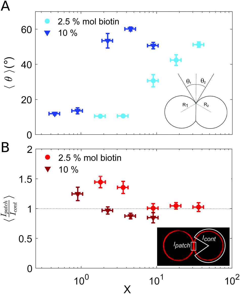Fig. 3 Characterization of vesicle doublets, as a function of the ligand-to-receptor ratio, X. (A) Contact angle (θ) of vesicle doublets, as a function of X. The contact angle was computed by averaging the two contact angles of the doublet (θ₁ and θ₂). The number of doublets analyzed for all conditions was set to N = 20 ± 4. The displayed values correspond to the mean, with the standard error as the error bars (error bars smaller than the symbol size are not displayed). In order to highlight the dispersion of the data a representation in a box-plot form is provided in the ESI.† (B) Fluorescence intensity at the vesicle–vesicle patch normalized by the intensity at the vesicle contour. The fluorescence was provided by SA molecules present on vesicle membranes. Doublets were imaged at their equatorial plane using confocal microscopy. Two different biotin contents were used: 2.5 and 10% mol. Vesicle volume fraction was set to 0.25% v/v (which corresponded to a total vesicle volume of 2.5 × 10⁸ μm³). The number of doublets analyzed for all conditions was set to N = 10 ± 4. The displayed values correspond to the mean, with the standard error as the error bars. A horizontal line at 〈I_patch/I_cont〉 = 1 is included as a guide to the eye.

3.2 Adhesive vesicle properties

3.2.1 Ligand–receptor density on vesicle membranes. In order to ensure that the targeted molar fraction of biotin-lipids was effectively incorporated into GUV membranes, fluorescence quantification of vesicle contours was performed in confocal microscopy. For this, we prepared vesicles with a fluorescent analog of the biotin-PEG(2000)-DSPE molecule, in which the biotin head was replaced with a carboxyfluorescein (CF) group³⁰ thus enabling quantification with fluorescence imaging, using the same molar lipid percentages of 1.25, 2.5, 5 and 10% mol. Since CF is emitting at 515 nm (green), for this set of experiments we marked the vesicle membranes with Rhodamine-lipid, emitting at 583 nm (red), at a fixed Rhod-lip/EggPC molar ratio of 1%, and that we used as a reference intensity value. We measured the fluorescence intensity of both the CF-green molecule and the red Rhodamine-lipid. The intensity ratio of both signals increased linearly with the CF molar percentage within experimental error (data is available at the ESI†). This suggests that the CF-lipid/Egg-PC ratio in the membrane corresponds to the lipid preparation used for the electroformation, and we expect the same behavior for biotinylated lipids.

Another important quantification concerns the number of (fluorescent) SA molecules bound to the outer membrane leaflet of the vesicles. For this, we quantified the fluorescence intensity of vesicle contours at SA saturating conditions, corresponding to the maximum fluorescence intensity obtained on the membrane when increasing the SA concentration in solution. The saturation intensity obtained for vesicles containing 10% mol biotin-lipid was only about two times larger than the values obtained for vesicles at 2.5% mol. In the following, we establish relation between this fluorescence intensity to the surface density of SA molecules bound to biotin-lipids on the vesicle membranes. We can estimate the surface density of biotin-lipids (Γ_b) taking into account the molar ratio of biotin-lipids used in the lipid mixture, and the surface of a phospholipid (65 Ų). This leads to Γ_b = 3.85 × 10⁴ μm⁻² and 15.4 × 10⁴ μm⁻² for vesicles containing 2.5% and 10% mol biotin respectively, or in other words, to a typical biotin-biotin distance on vesicle membranes of D_b = 5.1 nm and D_b = 2.5 nm respectively. The distance between biotin-lipids is, in both cases, comparable to the lateral size of SA molecules (of 4.8 nm and 5.5 nm, after the crystallographic data provided by Hendrickson et al.⁴⁹). For 2.5% mol biotin, one or two biotin-lipids can bind to a SA molecule. For 10% mol biotin, the distance between biotins is smaller than the lateral size of SA. Thus, SA molecules are dimerized, with two biotins bound per SA, and a fraction of biotin-lipids remains unbound. This would explain why the saturation intensity obtained for vesicles with 10% mol biotin-lipid was only about two times larger than the values obtained for vesicles at 2.5% mol. We have excluded in our interpretation the possibility for loop formation, in which more than two biotin-lipids from a same vesicle would bind to a SA molecule. The lateral size of PEG-2000 polymers for 2.5% and 10% mol biotin vesicles is L_PEG = 3.5 nm and 6.5 nm, respectively (which correspond to polymers in the mushroom and in the brush regimes).⁵⁰ Since the smallest lateral size of the SA molecule is L_SA = 4.8 nm, loop formation is geometrically hindered.

3.2.2 Adhesion of vesicle doublets. Experimentally, we measured the degree of vesicle–vesicle adhesion by determining the equilibrium contact angle (θ) between vesicles forming a doublet. In Fig. 3A we show the results obtained for the contact angle as a function of the ligand-to-receptor ratio, and for two different vesicles compositions (2.5% and 10% mol biotin-lipid). The values of contact angle, obtained at a given X value, display a significant dispersion. This may partly be attributed to the variability of electroformed GUVs, in terms of excess area, which can notably influence the contact angle of GUV doublets. In order to show the distribution of the contact angle values we provide in the ESI† a box-plot representation of the data. For 2.5% mol biotin, the smallest values of contact angles are θ ≃ 10°, corresponding to X ≤ 4. For very small contact angles (θ ≤ 15°), however, it was difficult to unambiguously distinguish experimentally vesicle-doublets from neighboring vesicles in close contact (but with no adhesion patch). A continuous increase in contact angle is observed for X ≥ 9. Doublets were clearly identified in this regime, as the vesicle membranes formed spherical caps. The largest values of the contact angles, θ ≃ 51°, correspond to the largest ligand-to-receptor ratios (X ≃ 36). For vesicles containing 10% mol biotin, the increase of the contact angle with X is steeper, and the curve is shifted towards smaller X values. The extent of the vesicle adhesion patch (and the contact angle) depends on the total number of bridges accumulated in it. At a given X ratio, vesicles with 10% mol biotin have four times more biotin available for bridges formation, and thus can display larger contact angles in vesicle-doublets than those containing 2.5% mol. For vesicles with 10% mol biotin, the maximum value obtained for the contact angle is slightly larger (θ ≃ 60°) than for 2.5%, which can also be attributed to a larger number of bridges formed in the adhesion patch. By increasing the SA concentration further (X > 5) the contact angle diminishes (this behavior is only observed for 10% mol biotin, since no larger X values could be reached experimentally for vesicles with 2.5%). We can interpret this downturn, as a situation being close to saturation of SA, for which almost all biotin sites would be bound to SA thus preventing further vesicle–vesicle adhesion and leading to a decrease in the extent of the adhesion patch.

Results for the fluorescence intensity of vesicle doublets are shown in Fig. 3B. The fluorescence signal corresponds to the SA fluorescent molecules attached to the vesicle membrane, so that we can relate the fluorescence intensity to the surface density of SA. The intensity of the adhesion patch (I_patch) is normalized by the fluorescence of the vesicle contour (I_cont). As shown in Fig. 3B, only for the lowest X values (X < 4 for 2.5% mol biotin and X < 1 for 10% mol), the intensity ratio is larger than one (X = 1.4 and 1.2, respectively). This implies that the intensity at the adhesion patch is larger than at the vesicle contour. These values correspond to slightly bound vesicles, with very small contact angles (Fig. 3A). In such conditions, only a few ligands are attached to membrane receptors, which can diffuse through the lipid membrane and get recruited at the adhesion patch, depleting the vesicle contour from ligands (fluorescent SA). This process is driven by the large binding affinity of the SA–biotin pair. The enrichment of the adhesion patch is in agreement with previous experimental results obtained using micropipette aspiration for small biotin molar percentages (up to 5% mol).³⁵ For larger X, the membrane coverage with fluorescent ligands was homogeneous all over the vesicles, with comparable values at the adhesion patch and at the vesicle contour. In this regime, the concentration of SA molecules may become sufficient to saturate all biotin sites (both on vesicle contours and in the adhesion patch), thus leading to intensity ratios close to one. Furthermore, Fenz et al.⁵¹ showed that biotin-lipids mobility was reduced when SA molecules are attached to them. In the limit of a high number of SA bound to biotin-lipids, an external high-viscosity layer of SA molecules might be formed increasing the hydrodynamic resistance to lipid mobility, limiting their recruitment at the contact zone in this regime. Unfortunately, our experimental setup does not allows us to assess the possible role of these kinetic effects. For 10% mol biotin vesicles and when X ≥ 4, the surface density of ligands in the vesicle contour may even exceed the density within the adhesion patch (I_patch/I_cont < 1). This X value corresponds to the downturn in contact angle (Fig. 3A), for which there exists a saturation of ligands in solution. We think this enhanced brightness observed for vesicle contours may be attributed to free ligands in solution attaching to vesicle contours at long time scales, after doublet formation. When the surface density of SA at the patch reaches its maximal (due to geometrical packing), any further diffusion of SA through the lipid membrane towards the patch is prevented. Note however that this argument is based on a time-dependent behavior which cannot be tested with our experimental setup. Alternatively, we could interpret this result based on additional entropic penalties experienced by linkers in the adhesion patch due to reduction of available configurational space, which has been described for DNA mediated adhesion.³¹ Compression of linkers within the adhesion patch upon vesicle–vesicle binding would lead to a decrease in their surface density in the patch, compared to the vesicle contour, which would result into a patch-to-contour intensity ratio lower than 1.

In the following, we address vesicle adhesion in the framework of thermodynamic equilibrium. This description, however, does not take into account dynamical process, which may play a non-negligible role in vesicle assembly. We can write the total free energy variation upon the formation of a vesicle doublet (ΔF) as the sum of an adhesion term (ΔF_adh) and an elastic term (ΔF_el) associated to membrane deformations,^40,52,53

ΔF = ΔF_adh + ΔF_el (1)

The adhesion term comprises a negative enthalpic contribution accounting for the formation of new ligand–receptor bonds in the adhesion patch and it is balanced by an entropic cost, related to the loss of degrees of freedom (translational and configurational) of surface-tethered receptors upon binding.^40,52,54 There exist, nonetheless, a negative entropic term associated to binding state multiplicity in multivalent systems, which favors binding^40,53,54 and which can strengthen the interaction. This combinatorial term is calculated by estimating all possible combinations of bounds formed between ligands and receptors. In our assembly experiments, binding multiplicity is provided by highly adhesive vesicles (which contain a large number of membrane receptors) and by the tetramic nature of SA molecules. The combinatorial term in multivalent biding increases faster than a simple linear addition of the binding energies of monovalent binders, due to a larger number of possible combinations between ligand and receptors.⁵⁴ Therefore, in our experiments this term may become significant for vesicles with a large content of biotinylated lipids. In particular, it may partly account for the steep increase in contact angle observed for 10% mol-biotin vesicles (Fig. 3A), compared to the smooth increase obtained for 2.5% mol-biotin ones. Membrane elastic deformations (ΔF_el) comprise both bending and stretching modes, and repulsion due to thermal membrane fluctuations. The latter can be neglected in the limit of strong adhesion.⁵⁵

In order to find the equilibrium doublet shape (and the equilibrium contact angle, θ_equil) the total free energy should be minimized with respect to the size of the adhesion patch. Solving the minimization problem is a challenging task, which is generally addressed numerically, or for limiting behaviors.^52,56 Ramachandran et al.⁵⁵ described vesicle–vesicle (LUV–LUV) adhesion theoretically in the strong adhesion limit, by introducing an interaction potential between two planar bilayers (W_P), which accounted for the binding energy density in the adhesion patch, and which was balanced by the elastic stretching of vesicle membranes (the bending energy term was neglected in this strong adhesion limit, and entropic contributions were not explicitly included in the model). Even though we use GUVs (instead of LUVs) we will discuss our results obtained for the contact angle (Fig. 3A) in the framework of this work.⁵⁵ The authors distinguished two main regimes for vesicle–vesicle adhesion: vesicles with constant volume and osmotically equilibrated deflated vesicles. Equilibrium contact angle was found to be independent of vesicle radii and to increase monotonically with the energy density, in the constant volume approach. In the osmotically equilibrated approach instead, the increase of contact angle with energy density was faster and was dependent on vesicle radius. We recovered small contact angles (θ < 15°) for low concentration of ligands (low X). We may interpret these low contact angles as corresponding to the constant volume approach, since vesicles are only slightly deformed, so that they can maintain their initial volume. By increasing the energy density (whether by increasing the biotin content on vesicle membranes or the number of ligands in solution, and thus X), we observed an increase of the equilibrium contact angle. This larger dependence could be attributed to the osmotically equilibrated regime. For such larger deformations, the increase in vesicle area leads to an increase of the vesicle pressure due to membrane tension, which is released by generating a flow of water through the semi-permeable membrane.

3.3 Controlling aggregate sizes

Setting a suitable ligand-to-receptor ratio is crucial for favoring the formation of prototissues of large sizes. As discussed in Section 3.2.2 for vesicle doublets, intermediate ligand-to-receptor ratios led to efficient vesicle–vesicle binding and should be thus also favored when designing vesicle prototissues with maximal sizes. This is shown in Fig. 4, where the mean size of vesicle aggregates (〈V_aggr〉) is shown (in log–log scale) as a function of X, for a constant number of vesicles in solution. The results of aggregate volumes provided in the figure are obtained from confocal microscopy images, after 3D-reconstruction. For these experiments, we used the Concentration method which favors vesicle–vesicle encounters and thus the formation of larger aggregates (compared to the Sedimentation protocol). As shown in Fig. 4, the mean aggregates size increases with X, until reaching a maximum aggregate value (for X ≃ 1). Increasing X further may result into a decrease of aggregate sizes caused by saturation of receptors by an excess of ligands in solution (as shown in the figure for vesicles containing 1.25% mol biotin-lipids). Biotin-lipid content on vesicle membranes also favored vesicle–vesicle adhesion, as it allowed a larger number of bridges to be formed between adjacent vesicles, and thus led to larger aggregate sizes, as observed in Fig. 4 for vesicles containing 1.25% up to 10% mol biotin. By using vesicles containing 10% mol biotin-lipid, we could reach aggregate sizes ranging on one order of magnitude (from 1.4 × 10⁴ μm³ up to 1.8 × 10⁵ μm³). We can estimate, as a first approximation (and disregarding interstitial fluid in between adjacent vesicles), the mean number of vesicles contained within the aggregates (〈M_aggr〉) by dividing the mean aggregate volume (〈V_aggr〉) by the mean vesicle volume (V_ves). We computed V_ves by taking into account the vesicle size distribution. This led to a mean aggregate number of 7 ≤ 〈M_aggr〉 ≤ 98 vesicles (shown in the right axis of Fig. 4).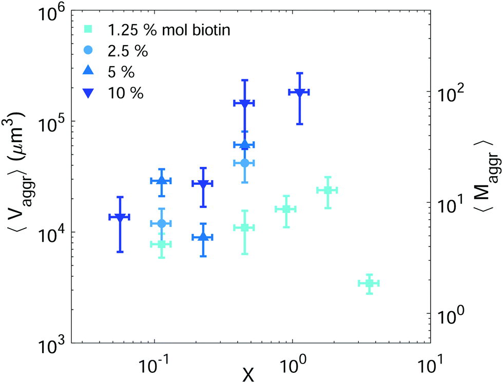

Fig. 4 Mean vesicle volume as a function of the ligand-to-receptor ratio, X. Different colors and symbols correspond to different biotin molar percentages on vesicle membranes (darker colors correspond to larger contents). Vesicle volume fraction was set to 5% (corresponding to a total vesicle volume of 5 × 10⁸ μm³). For all tested conditions the number of analyzed aggregates was set to N = 10 ± 4. The displayed values correspond to the mean and the error bars to the standard error.

The most effective way to control aggregate sizes was achieved by tuning the number of vesicles present in the assembly mixture. We show in Fig. 5 (in log–log scale) the mean (as well as the maximal) aggregate sizes as a function of the volume occupied by the total number of vesicles (V_tot), computed as the estimated total number of vesicles in solution times the mean vesicle volume (V_ves). In these experiments the assembly volume was kept constant, and the vesicle volume fraction was increased by increasing the total number of vesicles in solution. In order to maximize vesicle aggregate sizes we used vesicles containing 10% mol biotin-lipid, a ligand-to-receptor ratio favoring optimal binding (X = 0.45), and assembled them with the Concentration assembly protocol. For all conditions tested, we always obtained an ensemble of aggregates with diverse sizes. Aggregates of small sizes, and even single vesicles were always present. As the number of vesicles was increased, the maximal aggregate size was also increased, and so was the mean average size. By changing the total number of vesicles, mean aggregate sizes extended over more than three decades, 10⁴ μm³ ≤ 〈V_aggr〉 ≤ 1.5 × 10⁷ μm³, which corresponded to a mean aggregate number 5 ≤ 〈M_aggr〉 ≤ 8.1 × 10³. As the number of vesicles increased, aggregate sizes became larger because the number of building units was larger, but also because the vesicle–vesicle collision rate was increased. In the hypothetical case where all vesicles would be assembled into a unique aggregate, we would observe V_aggr ≃ V_tot. It is clear, that 〈V_aggr〉 ≪ V_tot. The mean aggregate volume increases more rapidly than linearly with the total vesicle volume (which corresponds to a power-law scaling with an exponent equal to 1), specially for large mean aggregate volumes (〈V_aggr〉 > 1.5 × 10⁵ μm³). Overall, the increase is compatible with a power-law scaling with exponent 2. In Fig. 5 we have included two lines with slopes 1 and 2, as guides to the eye. To the best of our knowledge, there is no theoretical framework available in the literature capable of rationalizing the observed trends. Vesicles assemble forming several aggregates of diverse sizes (as it is represented in Fig. 4 and 5). The size of vesicle aggregates may result from an intricate combination of different mechanisms, including kinetic effects taking place in vesicle assembly, or shearing forces which may eventually be exerted to the aggregates when removing them from the incubation tube by gentle pipetting, among others. Overall, this makes it difficult to predict theoretically the tendency of the mean aggregate size in terms of the total vesicle volume. We measured the sphericity (Φ), Φ = π^1/3(6V_aggr)^2/3/S_aggr, of vesicle aggregates (where S_aggr and V_aggr are the aggregate outer surface and the enclosed volume, respectively). Φ = 1 corresponds to a perfect sphere. As shown in the inset of Fig. 5, aggregates became more irregular in shape by increasing the total number of vesicles in solution. The increase of internal void regions, led to irregular 3d-aggregate morphologies, and could also partly account for the large increase observed for the mean aggregate size. Vesicle polydispersity is likely to have a role on the formation of irregular structures.^57,58 Besides, very large aggregates display planar shapes, which may be induced by their own weight, and which lead to small values of Φ.

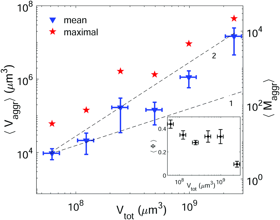Fig. 5 Mean (blue triangles) and maximal (red stars) aggregate sizes as a function of the total vesicle volume in solution (V_tot). Vesicle contained 10% mol biotin-lipids, and the ligand-to-receptor ratio was set to X = 0.45. For all tested conditions the number of analyzed aggregates was set to N = 15 ± 4. The displayed values correspond to the mean and the error bars to the standard error. Two lines with slopes 1 and 2 are included as guides to the eye. Inset: Mean sphericity (Φ) of the aggregates as a function of the total vesicle volume (V_tot).

In cell–cell adhesion, the biological activity, and in particular, active acto-myosin cortex is known to play a fundamental role which cannot be reproduced in our simplified biomimetic prototissue. Cortex contractility has an antagonistic effect to cell adhesion as it favors cell surface minimization (both mechanisms being interdependent), leading to different degrees of tissue compaction.^59,60 Attempts to perform cell aggregates have been addressed with the aim of modeling tumor progression,⁶¹ or for tissue engineering purposes in order to develop artificial organs or tissue transplants. Cell aggregates are constituted by the self-assembly of dispersed cells in suspension. Multicellular spheroids can grow up to typical volumes of 10⁹ μm³.⁶¹ As shown in Fig. 5, we can tune the GUV-aggregate sizes to attain the typical sizes of cellular spheroids, making them potential convenient biomimetic models. However, GUV aggregates display more irregular shapes. In multicellular aggregates round shapes are ensured by cell activity, allowing to explore more configurations and to reach more spherical shapes, minimizing their energy. Additionally, many biological tissues are constituted of cohesive cell monolayers. This is the case of epithelial tissues,⁵⁹ or germ layers.⁶² There is, therefore, an interest in developing 2d-biomimetic analogs, which enables to reproduce essential ingredients of these complex biological systems (which is addressed in the following section).

3.4 Prototissue morphology

3.4.1 3d-aggregates vs. 2d-monolayers. Aggregate morphology was qualitatively tuned by changing the incubation protocol. While Sedimentation and Concentration protocols led to rather globular shapes, in-plane Rotation during incubation induced the formation of vesicle monolayers. The formation of such artificial monolayers represents a simplified model system for epithelial cell monolayers (Fig. 6A). In panel B we show an example of a 2D-vesicle layer, analyzed with the Imaris Software. The reconstruction using this software shows that the prototissue is constituted of one single layer of vesicles. For comparison, we display in panel C a globular aggregate obtained at equivalent volume fraction.

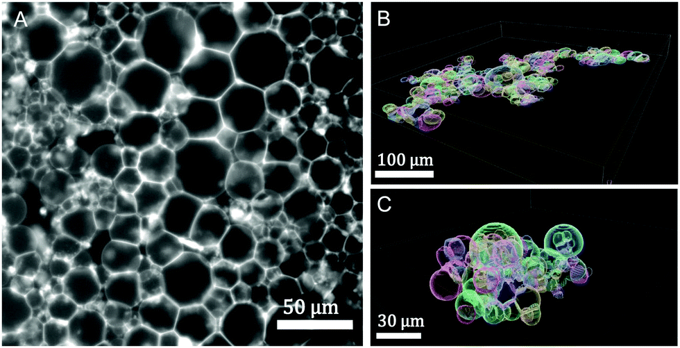Fig. 6 Prototissue morphologies: (A) 2d-epifluorescence image of a GUV monolayer, ressembling a tissue monolayer (2.5% mol biotin, X = 72.16, (R) assembly protocol). (B) 3d-reconstructed volume obtained from confocal images corresponding to a 2d-GUV-monolayer (10% mol biotin, X = 4.5, (R) assembly protocol). (C) 3d-reconstructed volume obtained from confocal images corresponding to a GUV globular aggregate (10% mol biotin, X = 0.45 (S) protocol). The vesicle volume fraction was set to 0.25% v/v in all assays.

3.4.2 Prototissue cohesion. Changing the number of receptors (biotin-lipids) on vesicle membranes also had an impact on aggregate cohesion. For a given X ratio, increasing the biotin content led to larger aggregates (as previously described for Fig. 4), which were in turn more compact. This trend can be observed in Fig. 7(A–D), in which two aggregates obtained with vesicles containing different biotin content are displayed. The change in aggregate cohesion is evidenced by the presence (or not) of interstitial voids between adjacent vesicles (as shown qualitatively in the 2D transverse slices of Fig. 7(C and D)). For 2.5% mol biotin vesicle–vesicle contacts were point-like. For 10% mol biotin vesicle contacts were larger (similarly to the behavior described for vesicle doublets) and the interstitial fluid was reduced. Experimentally, measuring the interstitial fluid in the interior of the aggregates was a challenging task. Instead, we measured the contact angle at the aggregate boundaries (θ_out) on a transverse slice, which is another indicator for aggregate cohesion.^18,60θ_out = (11.1 ± 1.2)° for vesicles with 2.5% mol biotin and θ_out = (30 ± 11)° for 10% mol. The latter, corresponds to the largest values of the outer contact angle that we observed for SA–biotin mediated vesicle aggregation (for all tested biotin contents and X ratios). We use this measure only as a qualitative indicator, as the contact angle may vary with the topology of the aggregate (coordination number of vesicles) and also due to vesicle polydispersity. A complete quantitative characterization of aggregate packing would require the full description of the topology of the microstructure (coordination number of each vesicle, number of neighbours, local packing fraction) based, for example, on space tessellation methods,^57,58 which is out of the scope of the present paper. Interestingly, vesicle–vesicle aggregation mediated by DNA complementary chains enabled the formation of aggregates with larger degrees of cohesion. Vesicle–vesicle adhesion was tuned by varying the concentration of the complementary DNA strands (in equimolar proportions) for a given vesicle volume fraction of vesicles of 0.125% v/v. The contact angles measured for vesicle doublets increased with DNA concentration up to maximal values comparable for those obtained when using the SA–biotin pair (Fig. 3). The cohesion of the vesicle aggregates was found to greatly vary with DNA concentration. In Fig. 7(E–H) we show two representative examples of two aggregates obtained at different DNA concentrations (32 nM, panels E and G, and 644 nM, panels F and H). At low DNA concentration the contacts between vesicles are of reduced size (θ_out = (32 ± 3)°) and interstitial voids are visible between neighboring vesicles. At larger DNA concentrations, the contacts are larger with almost no interstitial voids and the boundaries of the aggregate become smoother (θ_out = (68 ± 6)°). Such degrees of prototissue cohesion were never achieved with the biotin-SA pair.

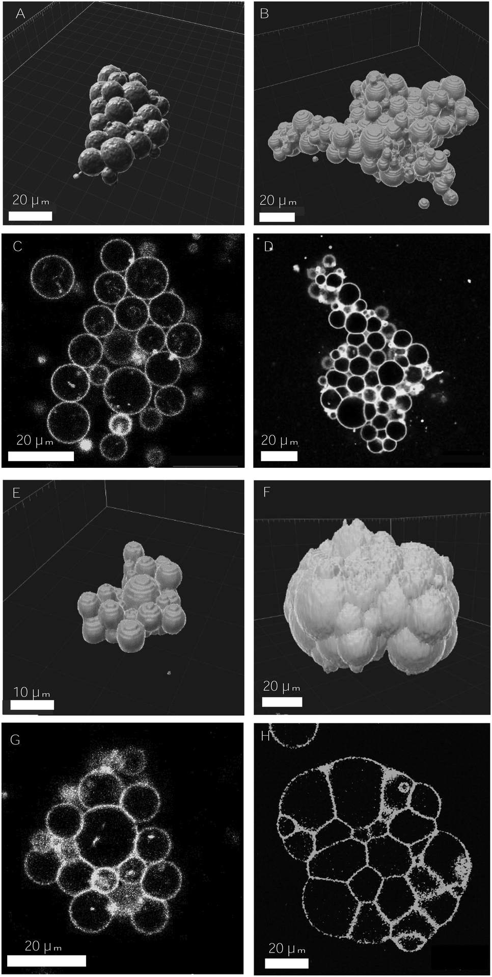Fig. 7 Examples of 3d-aggregates obtained with the SA–biotin pair (A–D) and DNA complementary strands (E–H) displaying different degrees of cohesion. 3d-reconstructed volume obtained from confocal images, using Imaris software (A, B and E, F), and 2d-confocal images (C, D and G, H). The concentration of receptors and ligands used in the assembly assays were the following: 2.5% mol biotin, X = 0.45 (A and C), 10% mol biotin, X = 1.12 (B and D), [DNA] = 32 nM (E and G), [DNA] = 644 nM (F and H). The volume fraction was set to 0.25% in A–D and to 0.125% in E–G.

In DNA-mediated assemblies there is a larger number of degrees of freedom for vesicle–vesicle binding. First, the typical binding energies of DNA complementary strands are half the energies for SA–biotin (35 vs. 18.3k_BT for the binding affinity in solution), and the length of the DNA spacer is three times larger than for PEG (14.5 nm vs. 6 nm) enabling to reach a larger number of accessible sites. Second, the anchoring of binders to lipid membranes is less strong (a cholesterol of 27 carbon groups vs. a DSPE with 41), favoring the detachment and reattachment of DNA strands from lipid bilayers.⁴⁸ In addition, the number of ligands per vesicle that can be reached using DNA strands is considerably larger, as there are no geometrical constraints caused by the presence of SA molecules around vesicle membranes, so that a larger number of bonds could be formed (disregarding the formation of loops). Altogether, we conceive that the larger flexibility offered by the DNA-mediated strategy allows ligands to rearrange in time, favoring larger intra-aggregate adhesion, and ultimately, more cohesive prototissues. Furthermore, DNA technology would be advantageous for the development of vesicle prototissues displaying programmable spatial heterogeneities. Recently, experiments based on the specificity and thermal reversibility of DNA interactions have made possible the synthesis of colloidal structures,⁶³ oil-in-water emulsions⁶⁴ and vesicle networks³¹ with programmable architectures. In particular DNA technology would be relevant for the development of heterotypic biomimetic 2D-monolayers displaying heterogeneities in both cell types and cell adhesions, with the aim of reproducing heterotypic boundaries observed, for example, in embryonic tissues separating ectoderm and mesoderm layers.⁶²

4 Conclusions

We have reported in this article the design of vesicle prototissues based on the controlled assembly of giant unilamellar vesicles, with the possibility of tuning their physical properties. Vesicle aggregation is mediated by specific adhesion interaction based on the streptavidin–biotin pair and its strength is tuned by changing the relative concentration of total SA molecules in solution to the total number of biotin molecules contained on vesicle membranes. We have identified an intermediate range of SA-to-biotin concentrations suitable for the formation of vesicle aggregation, which enables bridging between adjacent vesicles but low enough to prevent SA saturation of binding sites and consequently aggregation. By increasing biotin content on vesicle membranes, we have enhanced vesicle–vesicle adhesion and have favored the formation of aggregates of large sizes. Kinetics have a crucial role in the vesicle assembly process, as different dynamical mechanisms may take place simultaneously (frequency of vesicle–vesicle collisions, diffusion of free ligands in solution, and lateral diffusion of bound-ligands). For the range of high ligands and receptors concentrations that we have used, lateral diffusion through vesicle membranes is reduced and is not determinant for vesicle aggregation. We have shown, instead, that enhancing the probability for vesicle collisions, by bringing vesicles closer to each other, aggregate sizes can be efficiently controlled. Mean aggregate sizes can range from several vesicles up to 10⁴ vesicles. GUV-aggregates display an important degree of polydispersity in size and shapes. This polydispersity could be reduced making use, for example, of micropatterns with convenient geometries. The incubation method has also allowed us to control the geometry of prototissues, and in particular, to produce 2d-vesicle monolayers, which resemble the morphology of 2d-cell monolayers. Cohesion of vesicle prototissues increases with the number of receptors on vesicle membranes, and it has been maximized by using an alternative binding method, based on complementary DNA strands. We presume higher mobility of such ligands favors intra-aggregate organization of binders, leading to larger degrees of cohesion.

We believe designing biomimetic prototissues with significant sizes, an adjustable degree of cohesion, and different spatial configurations represents a promising tool for the study of cellular tissues. In particular, the vesicle prototissues designed in the present work could be used as biomimetic analogs for the modeling of multicellular spheroids or 2d-cell monolayers, which may help to deepen the understanding of tumor metastasis and morphogenesis.

Conflicts of interest

There are no conflicts to declare.

Acknowledgements

We acknowledge R. Merindol, F. Fagotto, F. Graner and L. L. Pontani for fruitful discussions, and M. In for a critical reading of the manuscript. We thank L. DiMichele for helpful advice on DNA vesicle assembly. We thank the assistance provided by E. Jublanc and V. Diackou from the microscopy platform of the University of Montpellier (MRI). This project is supported by the Labex NUMEV incorporated into the I-Site MUSE. The project has received additional funding from the Ecole Doctorale I2S (U. Montpellier).

Notes and references

1. A. Salehi-Reyhani, O. Ces and Y. Elani, Exp. Biol. Med., 2017, 242, 1309–1317.
2. J. W. Szostak, D. P. Bartel and J. W. Luisi, Nature, 2001, 409, 387–390.
3. P. Schwille, Science, 2011, 333, 1252–1254.
4. P. Schwille, J. Spatz, K. Landfester, E. Bodenschatz, S. Herminghaus, V. Sourjik, T. J. Erb, P. Bastiaens, R. Lipowsky, A. Hyman, P. Dabrock, J. C. Baret, T. Vidakovic-Koch, P. Bieling, R. Dimova, H. Mutschler, T. Robinson, T. Y. Tang, S. Wegner and K. Sundmacher, Angew. Chem., Int. Ed., 2018, 57, 13382–13392.
5. S. L. Veatch and S. L. Keller, Biophys. J., 2003, 85, 3074–3083.
6. S. Kretschmer, K. A. Ganzinger, H. G. Franquelim and P. Schwille, BMC Biol., 2019, 17, 1–10.
7. V. Noireaux and A. Libchaber, Proc. Natl. Acad. Sci. U. S. A., 2004, 101, 17669–17674.
8. L. L. Pontani, I. Jorjadze, V. Viasnoff and J. Brujic, Proc. Natl. Acad. Sci. U. S. A., 2012, 109, 9839–9844.
9. S. F. Fenz and K. Sengupta, Integr. Biol., 2012, 4, 982–995.
10. T. Trantidou, M. S. Friddin, A. Salehi-Reyhani, O. Ces and Y. Elani, Lab-on-a-Chip, 2018, 18, 2488–2509.
11. L.-L. L. Pontani, J. van der Gucht, G. Salbreux, J. Heuvingh, J.-F. F. Joanny and C. C. Sykes, Biophys. J., 2009, 96, 192–198.
12. D. Gonzalez-Rodriguez, K. Guevorkian, S. Douezan and F. Brochard-Wyart, Science, 2012, 338, 910–917.
13. F. Fagotto, Development, 2014, 141, 3303–3318.
14. T. Lecuit and L. Le Goff, Nature, 2007, 450, 189–192.
15. B. Aigouy, R. Farhadifar, D. B. Staple, A. Sagner, J. C. Röper, F. Jülicher and S. Eaton, Cell, 2010, 142, 773–786.
16. A. S. Smith and E. Sackmann, ChemPhysChem, 2009, 10, 66–78.
17. E. Sackmann and A. S. Smith, Soft Matter, 2014, 10, 1644–1659.
18. J. L. Maître and C. Heisenberg, Curr. Opin. Cell Biol., 2011, 23, 508–514.
19. H. Delanoë-Ayari, J. Brevier and D. Riveline, Soft Matter, 2011, 7, 824–829.
20. S. Mantri and K. Tanuj Sapra, Biochem. Soc. Trans., 2013, 41, 1159–1165.
21. H. Bayley, I. Cazimoglu and C. E. Hoskin, Emerging Top. Life Sci., 2019, 3, 615–622.
22. S. Chiruvolu, S. Walker, J. Israelachvili, F. J. Schmitt, D. Leckband and J. A. Zasadzinski, Science, 1994, 264, 1753–1756.
23. E. T. Kisak, M. T. Kennedy, D. Trommeshauser and J. A. Zasadzinski, Langmuir, 2000, 16, 2825–2831.
24. P. Vermette, S. Taylor, D. Dunstan and L. Meagher, Langmuir, 2002, 18, 505–511.
25. K. A. Burridge, M. A. Figa and J. Y. Wong, Langmuir, 2004, 20, 10252–10259.
26. N. Stuhr-Hansen, C. D. Vagianou and O. Blixt, Bioconjugate Chem., 2019, 30, 2156–2164.
27. S. Villringer, J. Madl, T. Sych, C. Manner, A. Imberty and W. Römer, Sci. Rep., 2018, 8, 1–11.
28. P. A. Beales and T. Kyle Vanderlick, J. Phys. Chem. A, 2007, 111, 12372–12380.
29. P. A. Beales and T. Kyle Vanderlick, Adv. Colloid Interface Sci., 2014, 207, 290–305.
30. M. Hadorn and P. E. Hotz, PLoS One, 2010, 5, e9886.
31. M. Mognetti, P. Cicuta and L. Di Michele, Rep. Prog. Phys., 2019, 82, 116601.
32. P. Carrara, P. Stano and P. L. Luisi, ChemBioChem, 2012, 13, 1497–1502.
33. T. P. De Souza, G. V. Bossa, P. Stano, F. Steiniger, S. May, P. L. Luisi and A. Fahr, Phys. Chem. Chem. Phys., 2017, 19, 20082–20092.
34. M. Wilchek, E. A. Bayer and O. Livnah, Immunol. Lett., 2006, 103, 27–32.
35. D. A. Noppl-Simson and D. Needham, Biophys. J., 1996, 70, 1391–1401.
36. P. Ratanabanangkoon, M. Gropper, R. Merkel, E. Sackmann and A. P. Gast, Langmuir, 2003, 19, 1054–1062.
37. A. Karlsson, R. Karlsson, M. Karlsson, A. S. Cans, A. Stromberg, F. Ryttsen and O. Orwar, Nat. Commun., 2001, 409, 150–152.
38. G. Bolognesi, M. S. Friddin, A. Salehi-Reyhani, N. E. Barlow, N. J. Brooks, O. Ces and Y. Elani, Nat. Commun., 2018, 9, 1–11.
39. Q. Li, S. Li, X. Zhang, W. Xu and X. Han, Nat. Commun., 2020, 11, 1–9.
40. L. Parolini, B. M. Mognetti, J. Kotar, E. Eiser, P. Cicuta and L. Di Michele, Nat. Commun., 2015, 6, 1–10.
41. P. Gobbo, A. J. Patil, M. Li, R. Harniman, W. H. Briscoe and S. Mann, Nat. Mater., 2018, 17, 1145–1153.
42. M. I. Angelova and D. S. Dimitrov, Faraday Discuss. Chem. Soc., 1986, 81, 303–311.
43. C. M. Warboys, M. Ghim and P. D. Weinberg, Atherosclerosis, 2019, 285, 170–177.
44. G. I. Bell, M. Dembo and P. Bongrand, Biophys. J., 1984, 45, 1051–1064.
45. E. A. Evans, Biophys. J., 1985, 48, 185–192.
46. F. Brochard-Wyart and P. G. De Gennes, Proc. Natl. Acad. Sci. U. S. A., 2002, 99, 7854–7859.
47. V. Caorsi, J. Lemière, C. Campillo, M. Bussonnier, J. Manzi, T. Betz, J. Plastino, K. Carvalho and C. Sykes, Soft Matter, 2016, 12, 6223–6231.
48. O. A. Amjad, B. M. Mognetti, P. Cicuta and L. Di Michele, Langmuir, 2017, 33, 1139–1146.
49. W. A. Hendrickson, A. Pähler, J. L. Smith, Y. Satow, E. A. Merritt and R. P. Phizackerley, Proc. Natl. Acad. Sci. U. S. A., 1989, 86, 2190–2194.
50. P. G. de Gennes, Macromolecules, 1980, 13, 1069–1075.
51. S. F. Fenz, R. Merkel and K. Sengupta, Langmuir, 2009, 25, 1074–1085.
52. A. S. Smith and U. Seifert, Phys. Rev. E: Stat., Nonlinear, Soft Matter Phys., 2005, 71, 1–11.
53. A. S. Smith and U. Seifert, Soft Matter, 2007, 3, 275–289.
54. F. J. Martinez-Veracoechea and M. E. Leunissen, Soft Matter, 2013, 9, 3213–3219.
55. A. Ramachandran, T. H. Anderson, L. G. Leal and J. N. Israelachvili, Langmuir, 2011, 27, 59–73.
56. U. Seifert and R. Lipowsky, Phys. Rev. A, 1990, 42, 4768–4771.
57. I. Jorjadze, L.-L. Pontani, K. A. Newhall and J. Brujic, Proc. Natl. Acad. Sci. U. S. A., 2011, 108, 4286–4291.
58. K. A. Newhall, L. L. Pontani, I. Jorjadze, S. Hilgenfeldt and J. Brujic, Phys. Rev. Lett., 2012, 108, 268001.
59. H. Turlier and J. L. Maître, Semin. Cell Dev. Biol., 2015, 47-48, 110–117.
60. M. L. Manning, R. A. Foty, M. S. Steinberg and E. M. Schoetz, Proc. Natl. Acad. Sci. U. S. A., 2010, 107, 12517–12522.
61. K. Alessandri, B. R. Sarangi, V. V. Gurchenkov, B. Sinha, T. R. Kiessling, L. Fetler, F. Rico, S. Scheuring, C. Lamaze, A. Simon, S. Geraldo, D. Vignjevic, H. Domejean, L. Rolland, A. Funfak, J. Bibette, N. Bremond, P. Nassoy, T. R. Kießling, L. Fetler, F. Rico, S. Scheuring, C. Lamaze, A. Simon, S. Geraldo, D. Vignjević, H. Doméjean, L. Rolland, A. Funfak, J. Bibette, N. Bremond and P. Nassoy, Proc. Natl. Acad. Sci. U. S. A., 2013, 110, 14843–14848.
62. F. Fagotto, Curr. Top. Dev. Biol., 2015, 112, 19–64.
63. M.-P. Valignat, O. Theodoly, J. C. Crocker, W. B. Russel and P. M. Chaikin, Proc. Natl. Acad. Sci. U. S. A., 2005, 102, 4225–4229.
64. L. Feng, L.-L. Pontani, R. Dreyfus, P. Chaikin and J. Brujic, Soft Matter, 2013, 9, 9816.

---

Footnotes

† Electronic supplementary information (ESI) available. See DOI: 10.1039/d1sm00336d

‡ Present address: Max Planck Institute of Colloids and Interfaces, Am Mühlenberg 1, 14476 Potsdam, Germany.

§ Present address: Potsdam University, Karl-Liebknecht-Str. 24-25, 14476 Potsdam, Germany.

---