DOI:
10.1039/D1SM00272D
(Tutorial Review)
Soft Matter, 2021,
17, 5645-5665
Continuum-scale modelling of polymer blends using the Cahn–Hilliard equation: transport and thermodynamics†
Received
22nd February 2021
, Accepted 31st May 2021
First published on 31st May 2021
Abstract
The Cahn–Hilliard equation is commonly used to study multi-component soft systems such as polymer blends at continuum scales. We first systematically explore various features of the equation system, which give rise to a deep connection between transport and thermodynamics-specifically that the Gibbs free energy of mixing function is central to formulating a well-posed model. Accordingly, we explore how thermodynamic models from three broad classes of approach (lattice-based, activity-based and perturbation methods) can be incorporated within the Cahn–Hilliard equation and examine how they impact the numerical solution for two model polymer blends, noting that although the analysis presented here is focused on binary mixtures, it is readily extensible to multi-component mixtures. It is observed that, although the predicted liquid–liquid interfacial tension is quite strongly affected, the choice of thermodynamic model has little influence on the development of the morphology.
1 Introduction
Polymer blends are of significance in many areas such as high-performance materials,1 organic photovoltaics,2 polymeric membranes3 and pharmaceutics.4 Most polymer blends tend to be incompatible, which results in blends consisting of multiple phases. As a result, the morphology of the blend, which is used to create a functional material, will have a significant impact on the material performance. The following list includes examples where the blend's morphological features are important in ensuring performance and it is certainly non-exhaustive.
(1) Organic solar cells require the polymer blends to adopt an interconnected/co-continuous morphology smaller than 20 nm.5
(2) The inclusion of rubber particles with an appropriate particle size distribution to polystyrene can improve the mechanical properties of the material.6
(3) The morphology of polymeric membranes can influence its separation capabilities in terms of selectivity and permeability. Specific examples of such internal structures include an asymmetric membrane structure7 or the orientation and distribution of the domains of a dispersed polymer species within a blend matrix.3
A common method to model the formation of these polymer blends at continuum length scales is to adopt a modified Cahn–Hilliard framework. This approach has previously been used to model binary8,9 or ternary polymer blends,6,10,11 or systems consisting of polymers and solvents.12 This framework can also be readily coupled to other equations such as the Stokes9 or Navier–Stokes equations13 for modelling more-complex processes involving flow-induced shearing effects.
The Cahn–Hilliard equation has multiple complexities from both a mathematical and physical standpoint. It is a fourth-order non-linear partial differential equation. The theoretical features and numerical solution of the Cahn–Hilliard equation and its modifications as outlined above is still an area of active research in applied mathematics and computational physics.14,15 Physically, the Cahn–Hilliard equation is fundamentally related to the thermodynamics of the system and this relation is captured in the Gibbs free energy of mixing function. An appreciation of non-ideal mass transport is also useful for understanding the Cahn–Hilliard equation. Typically, many studies employ a simple quartic polynomial, which has a double-well shape as the free energy function. While this does serve as a useful theoretical tool, it is difficult to obtain physically relevant information from such a potential. Therefore, more physically appropriate thermodynamic models need to be used.
In the case of mixtures containing polymers, the most common choice is the Flory–Huggins equation, which is a remarkably simple and powerful equation for which there is a wealth of supporting data from literature. However, there are a variety of more-advanced thermodynamic models that are better suited for specific systems or enable more-accurate modelling of complex systems that can be employed. To date, only a handful of studies have explored more-complex thermodynamic models, such as CALPHAD-based free-energy functions,16 the comparatively simple activity-coefficient model non-random two-liquid (NRTL)17,18 and free-energy functions suitable for mineralic systems,19 within the Cahn–Hilliard equation.
To the novice reader, the breadth and depth of the knowledge required to appreciate and use the Cahn–Hilliard model can be intimidating. Therefore, in the present work, we aim to introduce key features of the Cahn–Hilliard equation along with a robust introduction to a range of thermodynamic models that can be incorporated. We demonstrate how one can use this model to study polymer mixtures of interest. While the analysis is focused on mixtures containing polymers, it is readily extensible to other mixtures such as emulsions. The structure of the tutorial review is as follows: first, a phenomenological treatment of demixing is provided, then a derivation of the Cahn–Hilliard equation is presented. Subsequently, key features of the equation such as the mobility coefficient and gradient energy parameter are considered and we demonstrate their intimate connection to the Gibbs free energy of mixing function. We then explore various thermodynamic models that can be used to compute the free energy of mixing. Lastly, we explore the numerical solution of the Cahn–Hilliard equation in different settings such as considering how approximations to the free-energy expression and choice of mobility model impact the numerical solution. We also consider two model polymer blends; polystyrene–polybutadiene (PS/PB) and polystyrene–polymethylmethacrylate (PS/PMMA).
2 Phenomenology of demixing
To illustrate the nature of the demixing process, it is helpful to first consider the temperature–composition (T–x) diagram for a model system as shown in Fig. 1. The two-phase region is the region within the binodal curve and a homogeneous mixture that is quenched into this two-phase region will undergo phase separation to form two distinct phases. There are a variety of approaches to quench a mixture relevant for polymeric systems. These include: non-solvent induced phase separation (NIPS)20 where a non-solvent is added to a homogeneous polymer–solvent mixture to precipitate out the polymer, Thermally induced phase separation (TIPS)21 where the homogeneous mixture is prepared at a high temperature and cooled down to induce phase separation and lastly, polymerization-induced phase separation (PIPS)22 whereby miscible monomers are reacted to form a longer polymer chain that is immiscible.
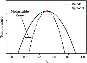 |
| | Fig. 1 Schematic of the T–x diagram for a system demonstrating phase separation. The point marked by the cross is the Upper Critical Solution Point (UCSP). | |
There are two mechanisms of demixing that need to be considered: “nucleation and growth” and spinodal decomposition. Nucleation and growth typically occurs within the metastable zone as indicated in Fig. 1. In the case of nucleation and growth, a large composition fluctuation i.e. the formation of a local region of high concentration of one species or a nucleus needs to form to trigger demixing. The nucleus then continues to grow as the mixture undergoes further demixing. In contrast, spinodal decomposition, also known as oiling out, involves smaller composition fluctuations. The reader is advised to review Favvas and Mitropoulos23 for a helpful one-dimensional illustration of the differences between the two mechanisms. Various figures throughout the present work also provide two-dimensional representations for both processes.
After the initial stages of demixing, the phenomenon of Ostwald ripening becomes noticeable. Ostwald ripening refers to the process of coarsening whereby larger domains grow at the expense of smaller domains.24 Through such coarsening, the system can further decrease the total free energy as the interfacial area decreases, which reduces the energy penalty associated with the formation of an interface. Examples of Ostwald ripening can be found throughout the manuscript, e.g.Fig. 9.
3 Cahn–Hilliard model
3.1 Model derivation
A modified Cahn–Hilliard model based on the work of Petrishcheva and Abart19 and Naumman and He10 is used to model the demixing of polymer blends. This approach can handle systems with orders of magnitude molecular-size difference e.g. polymers and solvents. Similar Cahn–Hilliard-type models have also been used to explore the morphological behavior of many-component polymer systems25 and also nanoparticle formation.12
The Cahn–Hilliard equation can be used to model uphill diffusion where transport occurs against a concentration gradient, thus the driving force is gradients in the chemical potential rather than concentration gradients. The flux ji of species i can be written as
| |  | (1) |
where
Mij is the mobility coefficient as expressed in the square symmetric mobility matrix
M, and
μj is the chemical potential of species
j. The flux of species
i can be expressed in terms of the difference in chemical potentials for additional convenience
i.e. μij =
μi −
μj:
| |  | (2) |
To obtain the transport equation for species i, the continuity equation is applied:
| |  | (3) |
where
t denotes time. For an
N component system, typically
N − 1 transport equations are defined and
ϕN for the last component is inferred from a material balance equation

, where
ϕi is the volume fraction of species
i. For a binary system with components 1 and 2, the transport equation for species 1 can then be written as:
| |  | (4) |
An expression for the chemical-potential difference, μij, can be obtained by considering the generalised N-component Landau–Ginzburg free-energy functional for inhomogeneous systems enclosed within a dimensionless volume Ṽ:
| |  | (5) |
where
GSystem is the total Gibbs energy of the system,
κi and
κij are the gradient energy parameters,

where
vref is a reference volume, typically the reference monomer volume, and
gm denotes the homogeneous contribution to the Gibbs free energy per monomer normalised such that:
| |  | (6) |
where
Nm is the number of monomers,
G is the homogeneous contribution to the total free energy,
kB is the Boltzmann constant, and
T is the temperature.
GSystem is scaled in the same manner as
eqn (6). For a binary system,
GSystem reduces to the following:
| |  | (7) |
It should be noted that the Landau–Ginzburg free-energy functional can be formulated using a free-energy density
gv which will have units of J m
−3 unscaled instead of
gm which is on a monomer basis and has units of J only. In such a case where
gv is used,
eqn (5) needs to formulated differently: the integral is defined over the actual volume
V instead of
Ṽ and the gradient energy parameter will have units of J m
−1 unscaled.
To evaluate μij, we compute the variational derivative on GSystem:
| |  | (8) |
which gives us the following expression for
μ12 in the binary system:
| |  | (9) |
Note that, because the homogeneous Gibbs free energy can be expressed as:
| |  | (10) |
where Δ
gmix,m denotes the normalised Gibbs free energy of mixing per monomer and the superscript * denotes a property related to pure species
i, in taking a derivative with respect to
ϕi and, subsequently, the gradient in equation
eqn (4), any information related to the pure species in equation
eqn (10) is lost without any loss of generality. As a result, for the purposes of the Cahn–Hilliard equation, only Δ
gmix,m needs to be provided.
At this stage, we can see that eqn (4) and (9) give us the fourth order partial differential equation (PDE) that constitutes our model equation. On first inspection, there are three components of the modified Cahn–Hilliard equation that would be “tunable” based on the specific polymers of interest:
(1) κ, the gradient energy parameter;
(2) M, the mobility coefficient;
(3) Δgmix,m, the Gibbs free energy of mixing.
As we will show in subsequent sections, κ and M are intimately related to Δgmix,m. Hence we shall first proceed with a discussion on the first two components.
3.2 Scaling
The following length x0 and time t0 scalings can be introduced to non-dimensionalise the model equations:| |  | (11) |
where M0 and L0 are the characteristic constant value for the mobility coefficient and the length respectively. We thus obtain the following non-dimensionalised model equations:| |  | (12) |
| |  | (13) |
3.3 Interfacial tension
A lasting consequence of the work of Cahn and Hilliard26 was the emergence of so-called square-gradient theory (SGT) as a widely used approach for the computation of interfacial tension (IFT), arising from their rediscovery of a result originally proposed in Dutch by van der Waals27 (see ref. 28 for an English translation). A helpful review of the different presentations of the theory has been provided by Carey et al.29
The solution of the Cahn–Hilliard model as outlined above can be employed to compute the IFT, denoted by Λ in the present work, of a system. Under the simplifying assumption of a planar interface, the concentrations vary in only one direction and the problem becomes one-dimensional. In the study of bulk thermodynamics where the interfacial arrangement, curvature and contact angle between phases are not of concern, this is a reasonable assumption. Following Naumman and He,30 we are then able to write the following expression for Λ:
| |  | (14) |
where
ρm is the monomer molar density and
R is the universal gas constant. In non-dimensional form,
eqn (14) can be written as:
| |  | (15) |
One may note from the form of eqn (14) and (15) that the gradient energy parameter is a key quantity in calculating the IFT.
4 Gradient energy parameter
The approach of Debye31 as extended by Ariyapadi and Nauman32 for multi-component systems, can be used to systematically evaluate the gradient energy parameters for a given expression of Δgmix,m. κ can be decomposed as follows:where the subscripts S and H denote the entropic and enthalpic contributions, respectively.26,32 For a given Δgmix,m expression such as the Flory–Huggins equation, a perturbation of the following form can be introduced:| |  | (17) |
where the * superscript refers to the value of ϕi with reference to a defined lattice point/central molecule and RG,i is the radius of gyration of species i. A perturbation expansion can then be performed and the resultant expansion, after discarding higher order terms, can be compared to the Landau–Ginzburg free energy functional to obtain κ by inspection. Often, Δgmix,m can be decomposed into an ideal (entropic) and residual (enthalpic) contribution from which one can obtain compact expressions for κS and κH separately. However, in the case where Δgmix,m cannot be decomposed, such as a quartic polynomial with a double-well, one would obtain only a single expression for κ, which can be quite complicated. A sample calculation for the case of a quartic polynomial is presented in the ESI.†
For a binary polymer blend using the Flory–Huggins equation, κS and κH can be written as follows:32
| |  | (18) |
| |  | (19) |
where
χ12 is the Flory–Huggins interaction parameter between species 1 and 2 and
Ni is the degree of polymerisation for species
i. We will outline in subsequent sections how
κ is computed in a tractable manner when more-complex thermodynamic models are used.
It is a common approximation to neglect κS when modelling polymer blends due to the large values of Ni which diminish its contribution.6,10 This also simplifies the computation due to the removal of an additional source of non-linearity in the model equation. As the focus of this study is on polymer blends, κS shall be neglected. However, in the case of polymer/solvent systems, the entropic contribution should not be so readily discarded as it can be significant.
We also note that within this model formulation, RG,i for the polymer species is treated as a constant and used as the length scale L0. Whilst it is true that RG can have a temperature and composition dependence, without a suitable expression in terms of model variables i.e. ϕ or T in the event temperature is considered, it is not possible to capture this physics in the model. Nonetheless, experimental morphology data has been replicated in previous work without accounting for these effects.30
5 Mobility coefficient
The mobility coefficients Mij are subject to the following constraints due to the Onsager reciprocal relationships and to account for interdiffusion respectively.19| |  | (20) |
Correspondingly, M can be written as follows for a binary system:19| |  | (21) |
The interested reader is advised to review Petrishcheva and Abart19 for a discussion on the ternary and multi-component cases.
There have been a variety of models for the mobility, but many of them are centered around the form of eqn (22).13,33–35 This can be understood from considering diffusion in non-ideal mixtures.19,30
| |  | (22) |
where
![[scr D, script letter D]](https://www.rsc.org/images/entities/char_e523.gif) ij
ij is the effective diffusion coefficient which can be written as follows:
19,30,35| |  | (23) |
where
Dij is the interdiffusion coefficient. If a suitable form of
Dij that accounts for temperature and composition dependence is available, such as in the case of accounting for the “fast” and “slow” models relevant to polymer–solvent systems,
35 it can be captured in this representation. Therefore, efforts to formulate a suitable mobility model should be focused on accurately evaluating
Dij.
At this stage, we should note some important conceptual features of the mobility coefficient. First, the introduction of the composition dependence in the form of the ϕi(1 − ϕi) term serves to restrict mass transport to the interface region which is physically accurate as interdiffusion cannot occur in regions where there is only a single species.19,30 Second, at the Spinodal where  ,
, ![[scr D, script letter D]](https://www.rsc.org/images/entities/char_e523.gif) ij and ji will be zero. This can be understood by further exploring the flux expression for a binary mixture where κ = 0:
ij and ji will be zero. This can be understood by further exploring the flux expression for a binary mixture where κ = 0:
| |  | (24) |
It can be seen in
eqn (24) that at the spinodal, the flux will be zero. Last, within the spinodal,
![[scr D, script letter D]](https://www.rsc.org/images/entities/char_e523.gif) ij
ij < 0 which correctly reflects the case of uphill diffusion as previously discussed. Correspondingly,
κ needs to be accounted for in the flux expression.
Often, in isothermal cases, Dij is taken as a constant and treated as the scaling for Mij, resulting in the following expression for M12 which has been used in studies involving polymer blends:6,8,10,11
Conceptually similar mobility models have also been employed for polymer solutions.
36,37
Another common approach is to assume a constant mobility38 and upon scaling, the following expression is obtained:
| | ![[M with combining tilde]](https://www.rsc.org/images/entities/i_char_004d_0303.gif) 12 = 1. 12 = 1. | (26) |
As we will show in the results section, the morphology obtained from numerical simulation is not impacted by using either
eqn (25) or
eqn (26). Manzananrez
et al.35 also demonstrated that, while different mobility models result in a similar morphology, the system dynamics as captured by the domain scaling growth laws can vary.
For completeness, there are a variety of other mobility models considered in the literature which are relevant for polymeric systems that build on eqn (22).35,39 Other approaches to capture dynamics related to glass-transition in systems, particularly with a polymer and solvent, have also been explored in the literature.40,41 The interested reader is advised to look through the various citations included in this section for additional detail.
6 Thermodynamic models for Δgmix,m
In this section, we give an overview of some of the different approaches available to obtain the Gibbs free energy of mixing for polymer blends which can be used within the Cahn–Hilliard equation. Most approaches discussed here obtain the Gibbs free energy of mixing in molar units, Δgmix, whilst eqn (77) requires it in per monomer units. Using a geometric average of the degree of polymerisation of the polymers, one can convert between the two:| |  | (27) |
6.1 Lattice-based approaches: Flory–Huggins equation
In adopting a lattice-based model, one considers how the polymer molecules can be arranged on a lattice; this enables the derivation of a thermodynamic model of the system through various means such as a mean-field approximation. The most relevant and common equation in this category for polymers is the Flory–Huggins equation,42 which expresses the dimensionless Gibbs free energy of mixing per monomer volume in terms of volume fractions as follows:| |  | (28) |
where Vi is the molar volume of species i, vref is the reference monomer volume, and Δgmix,v is the Gibbs free energy of mixing per monomer volume normalised in a similar way to eqn (6). For a binary system, eqn (28) can be written as:| |  | (29) |
It is possible to re-arrange equation eqn (29) to express the Flory–Huggins equation in monomer units, which is denoted by the subscript m:| |  | (30) |
where Ni is the degree of polymerisation of species i, often taken to be the number of monomers in species i. Eqn (30) is the form of the Flory–Huggins equation that is incorporated into the Cahn–Hilliard equation.
As implementing a model capable of predicting the behaviour of a wide variety of polymer blends is desirable, the present work has made various attempts to use generalisable approaches where possible. Specific to the Flory–Huggins equation, the approach used in in this work estimates χ12 using the method employed by Hildebrand and Scott43
| |  | (31) |
where
δi is the Hildebrand solubility parameter of species
i and can be obtained from sources such as Barton.
44 Other possible approaches include using the Hansen solubility parameters
45 or performing molecular simulations.
46,47
6.2 Activity-based approaches: UNIFAC-FV
A common method for simple molecules such as short alkanes and other organic compounds is the use of activity-coefficient methods48 to estimate and predict thermophysical properties such as liquid–liquid equilibrium (LLE). These methods include NRTL49 and UNIFAC/UNIQUAC.48 Such approaches have been adapted for use in polymer–solvent systems50 and with polymer blends, albeit with certain modifications.51,52
We are able to write down the following expression relating the normalised Gibbs free energy of mixing per mole to the ideal and excess contributions:
| | | Δgmix(x1) = Δgidealmix(x1) + Δgexcessmix(x1), | (32) |
where
| | Δgidealmix(x1) = x1![[thin space (1/6-em)]](https://www.rsc.org/images/entities/char_2009.gif) ln ln![[thin space (1/6-em)]](https://www.rsc.org/images/entities/char_2009.gif) x1 + (1 − x1)ln(1 − x1) x1 + (1 − x1)ln(1 − x1) | (33) |
and
| | Δgexcessmix(x1) = x1![[thin space (1/6-em)]](https://www.rsc.org/images/entities/char_2009.gif) ln ln![[thin space (1/6-em)]](https://www.rsc.org/images/entities/char_2009.gif) γ1 + (1 − x1)ln γ1 + (1 − x1)ln![[thin space (1/6-em)]](https://www.rsc.org/images/entities/char_2009.gif) γ2; γ2; | (34) |
here,
γi is the activity coefficient of species
i. Whilst the Cahn–Hilliard equation is expressed in terms of the volume fractions, activity-coefficient models tend to be expressed in terms of mole fractions. We can easily convert between the two:
| |  | (35) |
where
Vi is calculated using a reference density at a specified temperature and the thermal expansion coefficient, which can be obtained from literature.
53
The challenge for evaluating the Gibbs energy of mixing for a system now becomes an issue of evaluating the activity coefficient of the polymer molecules. The choice of a UNIFAC-based approach is desirable because of the predictive capabilities of such a group-contribution method, which requires only knowledge of the chemical structure of the species present. The UNIFAC-FV model used by Belfiore et al.51 with modifications from Thomas and Eckert54 can be used for polymer blends. The UNIFAC-FV model introduces a free-volume correction to the standard UNIFAC model to account for species with different molecular sizes.51,55 We are able to break down the activity coefficient into combinatorial, free-volume and residual contributions:
| | ln![[thin space (1/6-em)]](https://www.rsc.org/images/entities/char_2009.gif) γi = ln γi = ln![[thin space (1/6-em)]](https://www.rsc.org/images/entities/char_2009.gif) γcombinatoriali + ln γcombinatoriali + ln![[thin space (1/6-em)]](https://www.rsc.org/images/entities/char_2009.gif) γfree γfree![[thin space (1/6-em)]](https://www.rsc.org/images/entities/char_2009.gif) volumei + ln volumei + ln![[thin space (1/6-em)]](https://www.rsc.org/images/entities/char_2009.gif) γresiduali, γresiduali, | (36) |
The combinatorial contribution can be given as follows:
| |  | (37) |
where
ϕsegi refers to the segment fraction, which for a binary system is defined as:
| |  | (38) |
ri is the van der Waals volume of species
i and is defined as follows:
| |  | (39) |
where
vik is the number of groups of type
k in molecule
i and
Rk is the group volume which can be obtained from Gemhling
et al.56
The free-volume contribution can be written as follows:55
| | 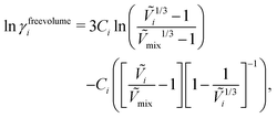 | (40) |
where
Ṽi is the reduced volume of species
i, the subscript “mix” refers to the mixture and the constant
Ci is related to the number of external degrees of freedom per molecule of
i.
55 Interested readers are advised to refer to the work of Iwai and Arai
57 and Bonner and Prausnitz
58 for more information and data related to
Ci for various polymers. The reduced volume terms can be written as follows:
| |  | (41) |
where
b is a constant with a value of 1.28 and
wi is the weight fraction of species
i.
The residual contribution can be written as follows:
| |  | (42) |
where
Γk is the residual activity of group
k in the mixture and
Γ(i)k is the residual activity of group
k in a pure solution;
Γk can be written as follows:
| |  | (43) |
where
Qk is the molar group volume parameter of group
k and can be obtained from sources such as Gemhling
et al.,
56Hm is the area fraction of group
m and
ψmn captures the intramolecular and intermolecular interaction energies between the various functional groups.
Hm is written as:
| |  | (44) |
where
Xm is the group mole fraction and can be written as follows:
| |  | (45) |
ψmn can be written as follows:
| |  | (46) |
where the values for
amn are tabulated in sources such as Gemhling
et al.;
56 ln
![[thin space (1/6-em)]](https://www.rsc.org/images/entities/char_2009.gif) Γ(i)k
Γ(i)k is calculated in a similar manner following
eqn (43) and (46) with the modification of
xi = 1 in
eqn (45) as the solution consists of a single species and the sums in
eqn (43) and (44) include only groups in the pure polymer.
6.3 Thermodynamic perturbation approaches: PC-SAFT
The final approaches discussed here are approaches based on the Statistical Associating Fluid Theory (SAFT);59,60 the SAFT equation of state is capable of capturing the properties of polymer–solvent mixtures by modelling each of these fluids as chains of equal-sized hard-spherical segments with either simple dispersive interactions or highly directional association sites. Molecules within the SAFT framework are typically described by the number of coarse-grained segments, m, comprising the chain that represents the molecule, the segment diameter, σ, and the segment energy (or the depth of the pair potential between individual segments of molecule), ε.
Many variants of the SAFT equation of state have been developed, some of which have been previously applied to polymer systems. Examples include soft-SAFT61 and, more recently, SAFT-γ Mie62 which, as a group-contribution approach,63 has the potential to be extended to a range of polymer systems. However, in this study, we focus on the Perturbed Chain-SAFT (PC-SAFT)64 equation of state, which, out of all the existing SAFT equations of state to date, has seen the most usage in the context of polymer systems.65–67 This equation allows one to obtain the reduced residual Helmholtz free-energy contributions as a function of T, V and x, from which physical properties can be derived:
| | | ares = aHC + adisp. + aassoc., | (47) |
where
a is the normalised Helmholtz free energy:
| |  | (48) |
The Helmholtz free-energy contributions can be decomposed in terms of the additive function of the hard-chain reference system contribution,
aHC, the dispersion contribution,
adisp. and the association contribution,
aassoc.
The hard-chain reference system contribution of the mixture, aHC, is determined by:
| |  | (49) |
where
![[m with combining macron]](https://www.rsc.org/images/entities/i_char_006d_0304.gif)
is the mean segment number given by:
| |  | (50) |
and
mi corresponds to the number of spherical segments present in the chain representing component
i.
aHC is likely to play a significant role in modelling polymer blends, especially considering the typically large number of segments used to represent such species.
68
It should be noted that, in the case of polymers, the spherical segments do not represent the monomers present in a chain nor, therefore, does mi represent the number of monomers (in a chain of species i). Indeed, mi need not be an integer value. By obtaining the number of segments for species in same homologous series through regression using experimental data, Kouskoumvekaki et al.69 have correlated the number of segments to the molecular weight of a species, resulting in a linear relationship between the two variables. From this relationship, it is possible to obtain the number of segments for polymers of any size within the same homologous series. aHS is the (dimensionless) Helmholtz free energy of a hard-sphere fluid per segment of the mixture:
| |  | (51) |
where
ζn is a reduced density that appears from Carnahan and Starling's hard-sphere free energy when it is modified to represent mixtures:
70,71| |  | (52) |
where,
ρ is the number density and
di corresponds to the temperature-dependent segment diameter of component
i given by:
| |  | (53) |
where
σi and
εi correspond to the size and energy parameters relating to molecule
i. Note that
ζ3 corresponds to the packing fraction, often denoted by
η.
gHSij is the radial distribution function of the hard-sphere fluid between species
i and
j, defined by:
70| |  | (54) |
The dispersive contributions are accounted for within the adisp term which consists of a second-order perturbation of the hard-chain reference system:
These are evaluated as:
| |  | (56) |
where
I1 and
I2 are power-series approximations in
η and
![[m with combining circumflex]](https://www.rsc.org/images/entities/i_char_006d_0302.gif)
of integrals involved in evaluating the perturbation terms:
| |  | (57) |
| |  | (58) |
Gross and Sadowski
72 have shown that the dependence of the coefficients
ai and
bi can be captured through universal correlations:
| |  | (59) |
| |  | (60) |
the parameters
aji and
bji are available from Gross and Sadowski.
64
C
1 corresponds to the compressibility expression, given by
| |  | (61) |
Finally, both

and

are molar averaged quantities of
m,
ε and
σ which include both like and unlike interactions between species (
ij). The unlike interactions are characterised by
σij and
εij, which are determined by the usual Lorentz–Bertholot-like combining rules:
| |  | (62) |
| |  | (63) |
where
kij is a binary interaction parameter relating to the interaction between segments
i and
j. A noteworthy observation when modelling polymer blends is that, relative to mixtures of low-molecular-weight species, the conditions of (calculated) LLE are very sensitive to the value of this parameter;
66 this is primarily because the interaction is segment-specific, thus, in longer chains (such as polymers), its effects are magnified.
The final contribution, ãassoc, accounts for highly directional associative interactions such as hydrogen bonding between sites on segments of species. This can be obtained from:
| |  | (64) |
where
nassoci is the number of types of sites on species
i,
ni,a is the number of sites of type
a on species
i and
Xi,a is the fraction of sites of type
a on species
i not bonded to any other site. The latter can be obtained by solving a set of mass-action equations:
| |  | (65) |
where
Δij,ab is the association strength between site of type
a on species
i and site of type
b on species
j. This can be obtained from:
| | | Δij,ab = gHSij(exp(εassoc.ij,ab/(kBT)) − 1)σijκij,ab, | (66) |
where
εassoc.ij,ab and
κij,ab are the potential well-depth and so-called bonding volume characterising the association between site of type
a on species
i and site of type
b on species
j. One additional complication of including this contribution is that
eqn (65) must be solved for iteratively (see ESI
† for further details). We note that the above formulation of the association term is different from that presented in chapman
et al.60's original work where the indices
a and
b denotes particular sites, rather than site types. The latter formulation is more-commonly used in recent SAFT publications.
Pure-component parameters for a variety of polymers are available in literature,65,73 as well as a group-contribution method66 specifically developed for polymer systems. However, obtaining the binary interaction parameter, kij, can be quite difficult and, as discussed previously, is very important for polymer blends. Typically, this parameter is obtained by adjustment using experimental data of properties involving components i and j such as vapour–liquid equilibrium properties, excess volumes of mixing, excess enthalpies of mixing.63,64 Alternatively, one can use combining rules (CR); many such rules have been proposed;74,75 among these, adopting the combining rule (CR) of Hudson and McCoubrey76 (and neglecting the minor differences in molecular ionisation potentials) leads to:
| |  | (67) |
Once all of the parameters are obtained, the Gibbs free energy and, by extension, the Gibbs free energy of mixing of a system can be calculated from:
| | g = aideal + ares + Z − ln![[thin space (1/6-em)]](https://www.rsc.org/images/entities/char_2009.gif) Z, Z, | (68) |
where
Z is the compressibility factor given by:
where the residual compressibility,
Zres factor can be obtained from:
| |  | (70) |
As a result, we can obtain the Gibbs free energy of mixing by re-arranging eqn (10). However, as PC-SAFT is derived within the canonical ensemble, it is not written explicitly in terms of the pressure, which requires the additional step of solving for the corresponding volume at a certain temperature and pressure. We note in passing that the molar volumes required to convert between the molar and volumetric fractions in eqn (35) can be obtained by finding the corresponding volume at a certain temperature and pressure for a pure species.
6.4 Redlich–Kister approximation
Simple thermodynamic models such as the Flory–Huggins and NRTL equations can easily be integrated within the Cahn–Hilliard equation, however, attempting to do so for more-complex models, such as the full PC-SAFT equation or the UNIFAC-FV equation, is not feasible in practice. This will likely be the case for many other such models; as a result, there is a need to approximate these such that they can then be used with the Cahn–Hilliard equation.
One can achieve this through the use of the Redlich–Kister equation, which is a convenient tool for expressing algebraically thermodynamic properties of solutions77 (volumes of mixing, Gibbs free energy of mixing, and so forth). The Gibbs free energy of mixing for an N-component mixture can be expressed as the sum of the ideal Gibbs free energy of mixing and the excess Gibbs free energy of mixing, Δgexcessmix(x1,x2,…,xN):
| |  | (71) |
Δ
gexcessmix(
x1,
x2,…,
xN) can be fitted to the Redlich–Kister polynomial equation:
77| |  | (72) |
where
Ci are the fitting parameters for the
kth-order polynomial fit, which can be systematically determined prior to solving the Cahn–Hilliard system for a given polymer blend. The order of the polynomial can be chosen to obtain a fit to desired level of accuracy within the domain [0,1] of
x1. We have found that the use of a 6th-order polynomial fit using 100 points within the domain is sufficient to fit the coefficients to the predictions made by these more-complicated models. This method is generalisable to most polymer blends and thermodynamic models.
6.5 Data-driven approaches
To conclude our discussion of thermodynamic models we draw attention to two classes of data-driven approach for studying the thermodynamics of mixtures. We do not consider these approaches explicitly in the remainder of our current study, but they are applicable to polymer blends and are mentioned here for completeness.
The first class of data-driven approaches involves constructing the equation of state for the system using machine-learning techniques. It is possible to then compute various properties of interest, including Δgmix,m. Employing such machine-learning-based approaches offers the advantage of being able to better capture the behaviour of the system due to the avoidance of a restrictive closed-form analytical expression for the molecular interactions or the equation of state itself.78,79 The interested reader is also advised to review Faúndez et al.80 for more information regarding the implementation of such an approach.
Another area of interest is the inverse problem for the Cahn–Hilliard equation. Broadly, the inverse problem can be understood as the process of using measurements to infer the value of the parameters or physics of a system.81 In recent work, the inverse problem for the Cahn–Hilliard equation has been explored; this has enabled the evaluation of the thermodynamics of the system from a few snapshots of the pattern forming process.82,83 This approach has particular utility for studying complex systems where there may be rich experimental data of the actual pattern-forming process, but formulating an accurate thermodynamic and/or transport model is non-trivial.
7 Numerical implementation
In this section, we give details on the numerical implementation of the PC-SAFT equation, the determination of liquid–liquid equilibria and interfacial tension for polymer blends using the various thermodynamic models and solution to the Cahn–Hilliard equation.
7.1 Pressure-dependence of PC-SAFT
As PC-SAFT is explicitly written in terms of the volume and temperature of the system, in order to obtain the relevant thermodynamic properties at a certain pressure (p0), temperature (T0) and composition (x0), assuming it is in a single phase, the following optimisation problem needs to be solved:| |  | (73) |
The solution to this optimisation will be the equivalent to the solution of:| |  | (74) |
in the present work this is solved using the least-squares solver in SciPy.84 We point out that implementing the SAFT association term within this formalism involves two layers of iterative numerical procedures, incurring considerable computational cost.
7.2 Determining liquid–liquid equilibria of polymer blends
Before even implementing any of the thermodynamic models within the Cahn–Hilliard equation, it is useful to obtain the phase diagram of the system to determine whether or not phase separation will occur. The conditions for thermodynamic equilibria are already well-known:| | | μi,α = μi,β ∀i ∈ {1,2}. | (77) |
where α and β are two hypothetical phases. Within the models discussed in Section 6, the temperature of the two phases can already be set and, in the case of the Flory–Huggins equation and UNIFAC-FV model, these models are pressure-independent. This leaves only eqn (77), which can be used to determine the composition of the two phases. von Solms et al.85 have proposed a method developed specifically for polymer systems and applied it to a variant86 of PC-SAFT; however, for the blends of interest here, we find that simply solving for the Gibbs Tangent Plane is adequate to solve for the compositions of the two phases.
7.3 Cahn–Hilliard model
In the present work, the non-dimensionalised Cahn–Hilliard equations given by eqn (12) and (13) are solved using the open-source finite-element-based declarative PDE solver FEniCS87 version 2019.1.0 using the Ocellaris 2019.1.0 Singularity container.88
All source terms are treated implicitly. The LU solver within the “NewtonSolver” environment is selected with an absolute tolerance of 10−16 and relative tolerance of 10−10. FEniCS and other solver codes also enables users to employ iterative methods which would be useful for larger and more complex systems. Periodic boundary conditions are applied. Details regarding the various simulation parameters can be found in Table 3. The initial condition of the ϕ1 field is set uniformly at the value of ϕ1,0 specified and perturbed with a random noise variable of magnitude 0.01 to trigger demixing.
The simulation data are then exported as a series of VTK files and post-processed using ParaView 5.6.1. The default “Cool to Warm” color scheme is used where reds and blues correspond to regions rich in species 1 and 2, respectively.
The interested reader is advised to refer to Wodo and Ganapathysubramanian89 for a comprehensive discussion on the numerical solution of the Cahn–Hilliard equation. Various open-source solvers in addition to FEniCS such as FiPy90,91 or MOOSE92 have been used to solve similar problems. PFHub93 is another excellent resource for problems involving phase-fields.
To compute the interfacial tension, a simplified one-dimensional simulation is carried out on a small domain and run until the system reaches equilibrium such that there is only a single interfacial region in the domain. The integral given by eqn (15) is computed at each timestep using the in-built integration functionality within FEniCS. It is also possible to evaluate the integral offline using ParaView or exporting the data and implementing a suitable quadrature scheme.
8 Validation
We consider two validation cases. The first case, “Case 1”, is from Vasishtha and Nauman,9 and the second, “Case 2”, is from He and Nauman.8 A summary of all the relevant material and simulation parameters can be found in Table 1. The simulations in the original study were performed in 2D, hence 2D simulations shall be exclusively employed in this section.
Table 1 Summary of simulation parameters for benchmarking test cases
| Test case |
ϕ
1,0
|
χ
12
|
N
1
|
N
2
|
x
0
|
t
0
|
![[t with combining tilde]](https://www.rsc.org/images/entities/i_char_0074_0303.gif) final
final
|
Domain size |
Mesh resolution |
Δ![[t with combining tilde]](https://www.rsc.org/images/entities/i_char_0074_0303.gif) |
| Case 1 |
0.5 |
0.0075 |
400 |
400 |
1.13 × 10⁻⁸ m |
6.4 × 10⁻⁶ s |
400![[thin space (1/6-em)]](https://www.rsc.org/images/entities/char_2009.gif) 000 000 |
128x0 |
128 × 128 |
2.0 |
| Case 2 |
0.77 |
0.004 |
800 |
1400 |
20 × 10−8 m |
4 × 10⁻⁶ s |
500![[thin space (1/6-em)]](https://www.rsc.org/images/entities/char_2009.gif) 000 000 |
40x0 |
80 × 80 |
2.0 |
This is also a convenient junction to consider two aspects of the model. First, as both validation cases employ the Flory–Huggins equation, we can consider how various approximations of the Flory–Huggins equation impact the numerical solution. Second, we can consider the impact of the mobility coefficient by using either eqn (25) or eqn (26).
We explore the following approximations to the Flory–Huggins equation:
(1) “Heat of Mixing” approximation94 where the entropic contribution of the Flory–Huggins equation is neglected: Δgmix,m ≈ χ12ϕ1(1 − ϕ1).
(2) Least-squares curve-fitted quartic polynomial approximation Δgmix,m ≈ f(ϕ1,ϕ12,ϕ13,ϕ14)
(3) Taylor series expansion of the full Flory–Huggins equation: 
(4) Taylor series expansion of the logarithmic terms only:  , where a(ϕ1,ϕ12,…) and b(ϕ1,ϕ12,…) are the expansions about ϕ1 = 0.5 for ln
![[thin space (1/6-em)]](https://www.rsc.org/images/entities/char_2009.gif) ϕ1 and ln(1 − ϕ1) respectively.
ϕ1 and ln(1 − ϕ1) respectively.
(5) Least-squares curve-fitted symmetric quartic double-well potential: Δgmix,m ≈ Aϕ12(1 − ϕ1)2.
A summary of the various runs and run labels can be found in Table 2.
Table 2 Summary of Flory–Huggins approximations and mobility models explored
| Mobility model |
Approximation |
Label |
|
Eqn (25)
|
Full Flory–Huggins |
Var-Full FH |
|
Eqn (26)
|
Full Flory–Huggins |
Con-Full FH |
|
Eqn (25)
|
Heat of mixing |
Var-Heatmix |
|
Eqn (26)
|
Heat of mixing |
Con-Heatmix |
|
Eqn (25)
|
4th order curve fit |
Var-Curvefit4 |
|
Eqn (26)
|
4th order curve fit |
Con-Curvefit4 |
|
Eqn (25)
|
Taylor expansion of logarithmic terms |
Var-LogTaylor |
|
Eqn (26)
|
Taylor expansion of logarithmic terms |
Con-LogTaylor |
|
Eqn (25)
|
Taylor expansion of full Flory–Huggins |
Var-FullTaylor |
|
Eqn (26)
|
Taylor expansion of full Flory–Huggins |
Con-FullTaylor |
|
Eqn (25)
|
Symmetric double well potential |
Var-Sym |
|
Eqn (26)
|
Symmetric double well potential |
Con-Sym |
Snapshots from our simulations are presented in Fig. 2; the snapshots of the benchmark simulations for comparison can be found in the cited ref. 8 and 9. Cases (a) and (c) in Fig. 2 correspond to the benchmarking simulation and we are able to reproduce those results reasonably well.
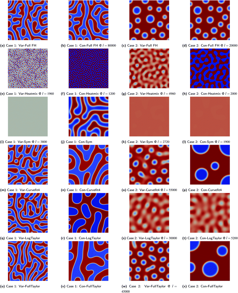 |
| | Fig. 2 Results of benchmarking cases for different Flory–Huggins approximations. The labels denote the adopted mobility model and Flory–Huggins approximation; see Table 2 for details. Each snapshot is taken at the end of the simulation (![[t with combining tilde]](https://www.rsc.org/images/entities/i_char_0074_0303.gif) final as given in Table 1), except where indicated. The colour bar range is restricted to between 0.0 and 1.0 for all images. final as given in Table 1), except where indicated. The colour bar range is restricted to between 0.0 and 1.0 for all images. | |
As previously discussed, the mobility model given by eqn (25), which restricts mass transfer to the interface, results in a slower rate of demixing and Ostwald ripening compared to the outcome when a constant mobility model given by eqn (26) is used. This is evident from how the runs in Fig. 2 using a constant mobility have much larger domains or have the same-sized domains at earlier times. The evolution of GSystem as given by eqn (7) which also represents the dynamical behaviour of the system can be seen in Fig. 3. We see that the morphology of the blend is not a function of mobility model, however, the dynamics can be impacted/unphysical if a suitable model is not used.30,35
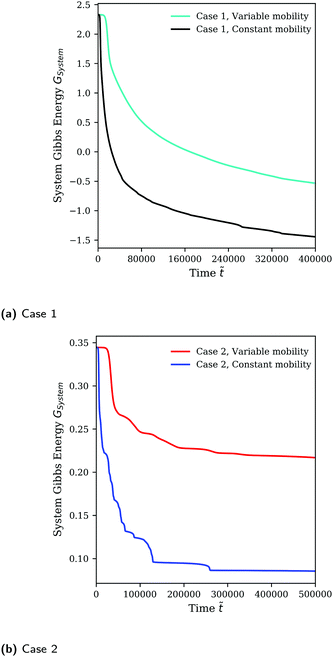 |
| | Fig. 3 Evolution of GSystem over time for Cases 1 and 2 (see Table 1) using the full Flory–Huggins equation as the homogeneous free energy expression. | |
The different approximations of the Flory–Huggins equation reveal a variety of different features and requirements of the free energy function. First, all the approximations resulted in numerical instability especially with the variable mobility model for Case 2. The exception to note is for the cases involving the symmetric double-well potential where 3/4 of the simulations terminated early not because of numerical instability during the emergence of a pattern, but rather because no pattern was forming.11
When the approximation does not have two minima within ϕ1 ∈ [0,1] such as in the case of heat-of-mixing” approximation or possibly having the minima outside the range ϕ1 ∈ [0,1] in the case of the 4th-order curve fit (an artifact arising from the regression process), the local mole fractions may not be conserved even though the total mole fraction is conserved. In the case of the heat-of-mixing approximation, the violation is significant with large values of ϕ1 at each cell e.g. ∼±1000 and larger. For the 4th-order curve fit approximation, the violation is much smaller, of order ∼5–10% from 0–1 for Case 2. The Cahn–Hilliard equation tracks GSystem which is decreasing monotonically by demixing (which decreases the homogeneous free energy) and Ostwald ripening which results in coarsening and a decrease in the interfacial area. In the case of the heat-of-mixing approximation, not only does ϕ1 locally diverge to large numbers comparatively quickly, but no Ostwald ripening is noticeable as the system is able to minimise the total Gibbs energy by generating increasingly large positive and negative cell mole fraction values which strongly reduces the homogeneous free energy, making the effects of domain coarsening minuscule in comparison.
These result indicates that, so long as the shape of the Gibbs free energy of mixing (along with its local minima) is appropriately captured by an approximation, the dynamic behaviour of the system should not be significantly different, thus demonstrating the validity of using a Redlich–Kister approximation of both PC-SAFT and UNIFAC-FV.
9 Test-cases
Within this section, PS/PMMA and PS/PB blends will be analysed in the context of the Cahn–Hilliard framework. These systems were selected primarily because of the wealth of literature available with respect to their blend morphology, phase behaviour and model parameters. Whilst all group-related parameters needed within the UNIFAC-FV model are readily available,48 the values of Ci (needed in eqn (40)) normalised for the polymer molecular weight for PS and PMMA can be obtained from Belfiore et al.51 The value of Ci for PB is obtained using the group-contribution method of Holten-andersen et al.95 Similarly, pure-component PC-SAFT parameters are readily available within the literature66,69 although binary-interaction parameters between polymers are obtained either from combining rules (eqn (67)) or regression to experimental data.
An additional benefit is that these polymer blends do not exhibit associating behaviour66 which would otherwise increase the complexity of the implementation of the PC-SAFT equation of state. Exploring the role of association and other complexities, such as diblock polymers, in impacting polymer-blend morphology is a topic of great interest.
In terms of blend morphologies, these are typically obtained from solvent-cast polymer films that undergo compositional quenching through flashing. These can be used as the benchmark for comparing experimental morphologies to those obtained from simulations.6,10,96 However, due to numerical instabilities, we are not able to directly reproduce the experimental data from works such as Ton-That et al.,97 Li et al.98 as the polymer chain lengths used in most experimental studies are prohibitively large. Consequently, the material and simulation parameters, which are outlined in Table 3, were selected so as to ensure that stable numerical solutions are obtained.
Table 3 Summary of material and simulation parameters for polymer blends of interest
| Polymer blend |
Thermodynamic model |
ϕ
1,0
|
N
1
|
N
2
|
R
G/m |
T/K |
D
12/m2 s |
![[t with combining tilde]](https://www.rsc.org/images/entities/i_char_0074_0303.gif) final
final
|
Domain size |
Mesh resolution |
Δ![[t with combining tilde]](https://www.rsc.org/images/entities/i_char_0074_0303.gif) |
| PS/PB |
F-H |
0.5 |
50 |
50 |
4.5 × 10⁻⁹ |
298 |
1 × 10⁻⁹ |
5000 |
100x0 |
500 × 500 |
1.0 |
| UNIFAC |
| PC-SAFT (CR) |
| PC-SAFT (Fitted) |
| PS/PMMA |
F-H |
0.25 |
500 |
500 |
1.4 × 10⁻⁸ |
472 |
1 × 10⁻¹¹ |
150![[thin space (1/6-em)]](https://www.rsc.org/images/entities/char_2009.gif) 000 000 |
100x0 |
500 × 500 |
1.0 |
| PS/PMMA |
UNIFAC |
0.25 |
25 |
25 |
3.2 × 10⁻⁹ |
472 |
1 × 10⁻⁹ |
7250 |
100x0 |
500 × 500 |
1.0 |
| PS/PMMA |
PC-SAFT (CR) |
0.25 |
25 |
25 |
3.2 × 10⁻⁹ |
472 |
1 × 10⁻⁹ |
10![[thin space (1/6-em)]](https://www.rsc.org/images/entities/char_2009.gif) 000 000 |
100x0 |
500 × 500 |
1.0 |
| PS/PMMA |
PC-SAFT (Fitted) |
0.25 |
100 |
100 |
6.4 × 10⁻⁹ |
472 |
1 × 10⁻¹¹ |
42![[thin space (1/6-em)]](https://www.rsc.org/images/entities/char_2009.gif) 000 000 |
100x0 |
500 × 500 |
1.0 |
In the first instance, we examine the polymer thermodynamics and phase behaviour obtained using the different approaches discussed in Section 6. Developing on this, we present simulation results for 1-3D cases to illustrate the type of morphology data that can be extracted. Typical values for the absolute time and length scales for the simulation are ![[scr O, script letter O]](https://www.rsc.org/images/entities/char_e52e.gif) (1 s) and
(1 s) and ![[scr O, script letter O]](https://www.rsc.org/images/entities/char_e52e.gif) (1 μm) respectively. We find that 2D simulations are adequate to describe the morphology of the system and present a variety of 2D results to compare the various thermodynamic models.
(1 μm) respectively. We find that 2D simulations are adequate to describe the morphology of the system and present a variety of 2D results to compare the various thermodynamic models.
9.1 Polymer thermodynamics and phase behaviour
It is useful to first analyse the predicted thermodynamic behaviour when using the different models prior to implementing these within the Cahn–Hilliard system to determine if we expect to observe phase splitting. The predicted LLE for oligomer blends of PS/PB and PS/PMMA can be observed in Fig. 4b. As we can see, for the same system, the different thermodynamic models can predict drastically different phase behaviour, highlighting the importance of selecting a model appropriately. This is particularly true when comparing the predictions made using the PC-SAFT equation; it is clear the binary interaction parameter, kij, has a very large influence on the predicted behaviour.
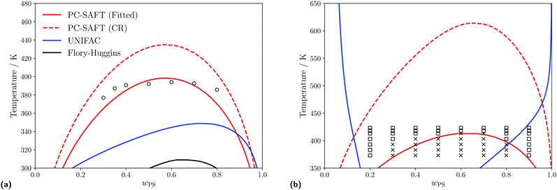 |
| | Fig. 4 Predicted liquid–liquid equilibria for different polymer blends of interest using the PC-SAFT with kij obtained from either the Hudson–McCoubrey combining rule (red, dashed) or fitting to experimental data (red, solid), UNIFAC (blue, solid) and Flory–Huggins (black, solid) equations. (a) Predicted LLE of a PS(1960)/PB(2350) blend. Empty circles represent experimental cloud points obtained from Lin et al.99 For PC-SAFT: kFittedij = −0.0003 and kCRij = 0.0001. (b) Predicted LLE of a PS(1390)/PMMA(6350) blend. Empty squares and crosses indicate conditions where a single phase or a two-phase split (respectively) is observed, (obtained from Kressler et al.100). For PCSAFT: kFittedij = 0.0160 and kCRij = 0.0180. | |
For the PS/PB blend as shown in Fig. 4a when using UNIFAC-FV or the Flory–Huggins equation, we do not accurately predict the experimental data, but do correctly predict that the polymer blend is of type I101,102 and exhibits an UCST within this temperature range. At lower temperatures (closer to the conditions which will be examined in this study), when using either UNIFAC-FV and PC-SAFT (using both methods to obtain kij), similar predictions for the compositions of the two phases are made.
For the PS/PMMA blend as shown in Fig. 4b, when using the various thermodynamic models, different phase behaviour is predicted. When using the Flory–Huggins equation, no phase split is predicted in the temperature range considered, whilst when using UNIFAC-FV, a type VI blend is predicted which is typically expected for longer chain lengths.101,103 However, the PS/PMMA blend is expected to be a type I blend,101,102 which is predicted when using PC-SAFT, regardless of which approach is used to obtain the kij parameter.
The substantial differences in predicted behaviour can perhaps be rationalised by the complex nature of the interactions between the PS and PMMA monomers, wherein the unlike interactions are strongly dissimilar from the like interactions, due to the presence of the polar ester groups present in PMMA. Adjusting the kij value using experimental data allows one to account implicitly for these interactions when using PC-SAFT but they are not well captured using the other equations, nor by PC-SAFT using the Hudson–McCoubrey combining rule, since this expression is based on an assumption that only London dispersion interactions are present.
For larger blends where experimental data are not available, we can, nevertheless, examine the Gibbs free energy of mixing for the polymer blends of interest using the various thermodynamics models to enhance our understanding of the thermodynamic behaviour. The Gibbs free energy of mixing for the blends of interest is shown in Fig. 5. For the PS/PB blend, the four models lead to rather similar predictions. This similarity can be linked to the previous observation that when these models are used, similar phase-behaviour is predicted (see Fig. 4a). In contrast to the Flory–Huggins equation, in spite of having equal chain lengths, using either UNIFAC-FV or PC-SAFT, asymmetric curves for the Gibbs free energy of mixing are generated. The maxima in the Gibbs free energy of mixing predicted using UNIFAC-FV is slightly shifted to a volumetric fraction of 0.6. For both approaches with PC-SAFT, the predicted minima are of different magnitude.
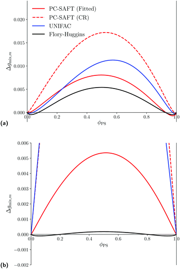 |
| | Fig. 5 Predicted Gibbs free energy of mixing at atmospheric pressure for different polymer blends of interest using the PC-SAFT with kij obtained using either eqn (67) (red, dashed) or by fitting using experimental LLE data (red, solid), UNIFAC (blue, solid) and Flory–Huggins (black, solid) equations. (a) Predicted Gibbs free energy of mixing for a of a PS/PB blend with N1 = N2 = 50, at T = 298 K. For PC-SAFT: kFittedij = −0.0014 and kCRij = −0.0001. (b) Predicted Gibbs free energy of mixing for a of a PS/PMMA blend with N1 = N2 = 500, at T = 472 K. For PC-SAFT: kFittedij = −0.0125 and kCRij = −0.0180. | |
On the other hand, analogous to the LLE for PS/PMMA, the four models lead to significantly different predictions for the Gibbs free energy of mixing for the PS/PMMA blend as shown in Fig. 5b. Values obtained using the Flory–Huggins equation are orders of magnitude smaller than those obtained using either UNIFAC-FV or PC-SAFT (Fitted), although, PC-SAFT, in either approach, can also be used to predict an almost symmetrical Gibbs free energy of mixing where the two phases are predicted to be almost pure PS and PMMA, respectively. One can also see that the Gibbs free energy of mixing also changes drastically when one uses a different value for kij in PC-SAFT, which likely a reflection of the different predicted UCST between the two approaches in Fig. 4b. In contrast to PC-SAFT and the Flory–Huggins equation, when UNIFAC-FV is used, a highly asymmetric Gibbs free energy of mixing is obtained where, not only is the maximum shifted towards 0.3, but the minima are of significantly different magnitudes. In addition, the location of these minima are quite asymmetrical as well, with one being close to pure PMMA and the latter only being at a volumetric fraction of 0.85, in contrast to the other models which all have minima close to almost-pure compositions. These drastic differences are expected to be reflected in the behaviour predicted by the Cahn–Hilliard system.
Overall, all thermodynamic models considered predict phase-splitting at the conditions considered; however, the composition at which these minima occur can be drastically different. The impact of this is examined in the subsequent section.
9.2 Interfacial tension
Before discussing our IFT calculations, it is important to reflect on the nature of SGT and its use in describing experimentally observed fluid–fluid IFTs. It has long been recognised that, used in traditional predictive fashion, the quality of the description of the IFT is lacking in quantitative accuracy.29,30,104 This stems from the calculation of the gradient energy parameter (or the influence parameter, its analogue in the vdW representation of the theory); see, for example, ref. 105 for a helpful summary of the literature on this point. Consequently, it is more usual to use SGT as a correlative approach to describe fluid–fluid IFT, rather than a predictive one, as we adopt in our current study. Indeed, the current popularity of the approach owes much to the works of Carey and co-workers29,106,107 who introduced two innovations to the modelling. The first was to use the (then) recently published Peng and Robinson equation of state108 to provide the fluid thermodynamics; in common with other cubic EoS, this equation is usually parameterized in such a way as to guarantee exact capture of experimental pure-component critical temperatures and pressures. The second, crucial advance was to “invert” the application of the theory by using experimental IFT data to back-calculate the influence parameter (the analogue of the gradient energy parameter in the vdW representation of SGT), instead of inferring it based on the molecular model.105 In other words, κ is taken as an adjustable parameter, leading to agreement between theory and experiment.109 In our current work, κ is not treated as adjustable; with this in mind, the provision of a good description of the IFT represents a stern test of our (predictive) approach.
The dependence of the IFT of PS/PMMA blends on PS molecular weight is explored, under isothermal conditions at T = 472 K, using experimental data from Anastasiasdis et al.110 as a reference; the number average molecular weight of the PMMA is 10![[thin space (1/6-em)]](https://www.rsc.org/images/entities/char_2009.gif) 000 Da. The descriptions obtained using the UNIFAC and PC-SAFT models are presented in Fig. 6. (The Flory–Huggins model is omitted from this discussion since it does not demonstrate phase splitting at the conditions considered, when using the Hildebrand solubility parameter approach to compute χ12.)
000 Da. The descriptions obtained using the UNIFAC and PC-SAFT models are presented in Fig. 6. (The Flory–Huggins model is omitted from this discussion since it does not demonstrate phase splitting at the conditions considered, when using the Hildebrand solubility parameter approach to compute χ12.)
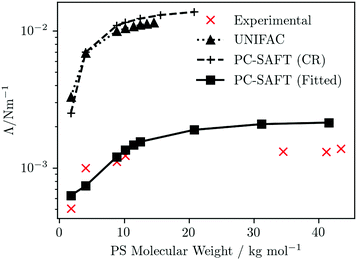 |
| | Fig. 6 PS-molecular-weight dependence of the interfacial tension of PS/PMMA(10![[thin space (1/6-em)]](https://www.rsc.org/images/entities/char_2009.gif) 000) blends at T = 472 K. Symbols represent predictions obtained using UNIFAC or PC-SAFT (as indicated) for the fluid thermodynamics (with connecting lines as a guide for the eye). The experimental data are taken from Anastasiadis et al.110 000) blends at T = 472 K. Symbols represent predictions obtained using UNIFAC or PC-SAFT (as indicated) for the fluid thermodynamics (with connecting lines as a guide for the eye). The experimental data are taken from Anastasiadis et al.110 | |
The qualitative trends from all three predictions reflect that of experiment, featuring a rapid increase at low PS molecular weight, plateauing to a near constant value at high PS molecular weight. However, quantitatively, significant differences are seen, depending which of the three approaches is used for the fluid thermodynamics. κ is sensitive to Δgmix; given the relative magnitudes of Δgmix obtained using the different approaches (see Fig. 5b) one would expect the IFTs predicted using UNIFAC and PC-SAFT (CR) to be larger than those using PC-SAFT (Fitted) and this is indeed what is observed. When using either UNIFAC or PC-SAFT (CR) to provide the thermodynamics, compared to experiment the IFT is overpredicted by approximately an order of magnitude; by contrast, the agreement between the predictions using PC-SAFT (Fitted) and experiment is rather good.
It is interesting to consider the relative success of the different predictions of IFT from an alternative perspective, provided by considering the differences between experimental and theoretical phase diagrams and, in particular, the locations of critical solution points. The IFT represents the energy cost to the system of sustaining an interface at the boundary between two coexisting phases; at a critical point, the distinction between the two phases disappears, whereby Λ ![[radiolysis arrow - arrow with voltage kink]](https://www.rsc.org/images/entities/char_e116.gif) 0 as the system approaches the critical point. A consequence of this is that, even if the dependencies of the IFT are well captured by the theory, the theoretical predictions of the IFT for a particular fluid should be quantitatively accurate only if the critical point of the model fluid (underlying the theory) coincides exactly with the experimental critical point. For example, if the critical temperatures differ, one should expect a systematic deviation between experimental and predicted IFTs as a function of temperature. This is not an issue for simple fluids and their mixtures, where an appropriate choice of EoS can ensure accurate agreement between theoretical and experimental critical temperatures and pressures. However, for more-complex mixtures, such as polymer blends, it becomes more difficult to capture critical points - indeed, experimental determinations of critical solution points may be unavailable – whereby it becomes an important consideration. Although we do not have computed and experimental phase diagrams of any of the PS/PMMA(10
0 as the system approaches the critical point. A consequence of this is that, even if the dependencies of the IFT are well captured by the theory, the theoretical predictions of the IFT for a particular fluid should be quantitatively accurate only if the critical point of the model fluid (underlying the theory) coincides exactly with the experimental critical point. For example, if the critical temperatures differ, one should expect a systematic deviation between experimental and predicted IFTs as a function of temperature. This is not an issue for simple fluids and their mixtures, where an appropriate choice of EoS can ensure accurate agreement between theoretical and experimental critical temperatures and pressures. However, for more-complex mixtures, such as polymer blends, it becomes more difficult to capture critical points - indeed, experimental determinations of critical solution points may be unavailable – whereby it becomes an important consideration. Although we do not have computed and experimental phase diagrams of any of the PS/PMMA(10![[thin space (1/6-em)]](https://www.rsc.org/images/entities/char_2009.gif) 000) blends considered in Fig. 6 available for comparison, one may expect a broadly similar picture to that provided in Fig. 4b, for the PS(1390)/PMMA(6350) blend. Reasonable quantitative agreement in the value of the UCST of the PS/PMMA blend is obtained using PC-SAFT (Fitted); this is reflected in the reasonable predictions of the IFT evidenced in Fig. 6. In contrast, the UCST is significantly overestimated using PC-SAFT (CR), while the UNIFAC description yields no UCST at all within the temperature range considered; indeed, the trend of the phase diagram appears to suggest a lower (rather than upper) critical solution point.
000) blends considered in Fig. 6 available for comparison, one may expect a broadly similar picture to that provided in Fig. 4b, for the PS(1390)/PMMA(6350) blend. Reasonable quantitative agreement in the value of the UCST of the PS/PMMA blend is obtained using PC-SAFT (Fitted); this is reflected in the reasonable predictions of the IFT evidenced in Fig. 6. In contrast, the UCST is significantly overestimated using PC-SAFT (CR), while the UNIFAC description yields no UCST at all within the temperature range considered; indeed, the trend of the phase diagram appears to suggest a lower (rather than upper) critical solution point.
As a final comment in relation to the IFTs, we note that for polymer mixtures at lower molecular weights, such as the mixtures considered within the first few data points of Fig. 6, the neglect of κS is a less-satisfactory approximation, which may impact on the quality of the IFT predictions. For those based on UNIFAC and PC-SAFT (CR), which are in any case quantitatively poor, this is not important but it may be a relevant consideration in relation to the predictions obtained using PC-SAFT (Fitted).
9.3 1–3D simulations
The dimensionality of the simulation is considered by exploring the PS/PB blend at different values of ϕ1,0 using the Flory–Huggins equation for simplicity. A lower mesh resolution (100 cells per vertex) is used to minimize computational expense especially for the 3D cases. As evident from the 2D case in Fig. 7 and 8, the lower mesh resolution does not compromise on the quality of the morphology obtained from the simulation.
 |
| | Fig. 7 1, 2 & 3D blend simulations for PS/PB blends at ϕ1,0 = 0.5. Snapshots at ![[t with combining tilde]](https://www.rsc.org/images/entities/i_char_0074_0303.gif) = 5000 are presented. In the case of the 3D simulation, the isosurface at ϕ1 = 0.5 is presented. = 5000 are presented. In the case of the 3D simulation, the isosurface at ϕ1 = 0.5 is presented. | |
 |
| | Fig. 8 1, 2 & 3D blend simulations for PS/PB blends at ϕ1,0 = 0.25. Snapshots at ![[t with combining tilde]](https://www.rsc.org/images/entities/i_char_0074_0303.gif) = 5000 are presented. In the case of the 3D simulation, the isosurface at ϕ1 = 0.5 is presented. = 5000 are presented. In the case of the 3D simulation, the isosurface at ϕ1 = 0.5 is presented. | |
Whilst it is clear that the 1D simulations are inadequate to properly understand the morphology of the system, 2D simulations are able to provide the necessary insight for these binary systems considering that the co-continuous morphology in Fig. 7 and the particulate morphology Fig. 8 are evident in the 2D case. We also note that the 2D PS/PB simulation at ϕ1 = 0.25 yields an almost identical morphological result to the PS/PMMA case subsequently presented which indicates that values of N1/N2 and χ12 do not significantly impact the morphology with the value of ϕ1 being the important factor in the symmetric case. This result is not entirely unexpected as there are only two phases present, which severely restricts the complexity of the observable morphologies. For ternary or multicomponent mixtures, the morphology can be significantly more complex10,11 and 3D simulations may be necessary to resolve important structural details.
9.4 2D simulations
As shown in Fig. 5 the magnitudes of Δgmix,m can vary significantly between the various thermodynamic models for the same mixture. As such, estimating the appropriate value of κ for each case is important as it is physically inappropriate to use the same value of κ when the Gibbs free energy of mixing function indicates that the interfacial energy significantly varies as well. If one were to obtain κ rigourously, this would involve the use of the method of Ariyapadi and Nauman,32 as previously discussed, which can result in an excessively complex expression for κ. When obtaining κ for the NRTL model, Zimmermann et al.18 used order-of-magnitude estimates. Other studies instead specified a constant value of κ in a semi-empirical fashion.13,111
To obtain a more-rigourous expression for κ whilst retaining the simplicity of the expressions given by ref. 32, we introduced a regression step at the start of the simulation which curve-fits the Flory–Huggins equation with χ12 as the free parameter to the computed values of Δgmix,m from a given thermodynamic model. This step yields an approximate value of χ12 which can then be passed into eqn (19). If both the Cahn–Hilliard model and thermodynamic equations were defined in terms of mole fractions, a similar estimation procedure could be carried out directly using a zeroth order Redlich–Kister expansion as the residual component for both the zeroth order Redlich–Kister equation and the Flory–Huggins equation are conceptually similar. Additional details on the estimation procedure with exemplar plots of the temperature dependence of κ can be found in the ESI.†
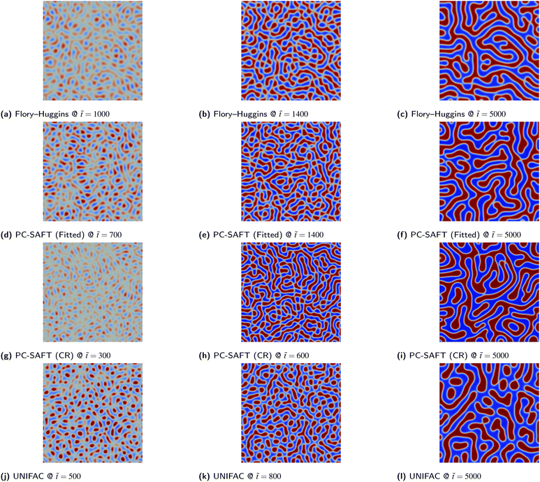
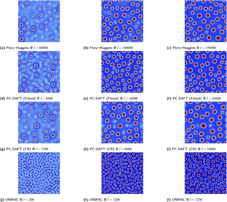
Consistently for both blends, the various thermodynamic models considered yield comparable results for the blend morphology. For PS/PB blends, both phases precipitate out simultaneously and a web-like co-continuous structure is formed. For PS/PMMA blends, the PS phase precipitates out first forming globular structures that undergo Ostwald ripening as time progresses. The resultant morphology for these binary systems arguably is more a function of the initial composition ϕ1,0 as opposed to the actual species present as discussed previously. The consistency of the morphology for PS/PMMA blends for the various Flory–Huggins and PC-SAFT is interesting as the values of N1 and N2 specified for the different equations varied significantly. The similarity in morphologies could also be attributed to the fact that, as shown in Fig. 5a, the values of Δgmix,m need to be comparable to the energies predicted by the Flory–Huggins equation for the simulation to be numerically stable. Hence, comparable free energy functions are being passed into the simulations. Whilst it would be desirable to compare systems with the same values of N1 and N2, this is challenging due to numerical instabilities.
10 Conclusions and outlook
It was the goal of this work to present how the Cahn–Hilliard equation can be applied to model polymer blends at a continuum scale. As demonstrated in the first few sections, the Gibbs free energy of mixing function Δgmix,m is central in formulating a well-posed model. To that end, we have provided an extensive overview of various thermodynamic models that can be employed to supply Δgmix,m, taking particular care to ensure consistent notation throughout. Even though the polymer blends we have explored with our approach are comparatively simple binary systems, the Cahn–Hilliard and thermodynamic models can all be readily extended, allowing our combined approach to be applied to multi-component blends, and to account for more-complex physics such as intermolecular association, and hydrodynamics.
Approximating Δgmix,m with functions of various forms and assuming a constant mobility coefficient does not impact the accuracy of the numerical solution of the Cahn–Hilliard equation, as long as the approximation captures the general shape of Δgmix,m. This result is essential for integrating UNIFAC or PC-SAFT into the Cahn–Hilliard equation, since a direct integration is computationally intractable due to the complexity of these thermodynamic models. Instead, by employing a Redlich–Kister equation, a high-accuracy approximation of Δgmix,m as predicted by the various thermodynamic models can be captured and passed into the Cahn–Hilliard model. Assuming a constant mobility results in a much faster rate of mass transfer, which adversely impacts the dynamics of the process. However, if one is interested only in the morphology, this need not be of concern. Adopting the Redlich–Kister approximation also allows for the gradient energy parameter to be estimated conveniently for the different thermodynamic models, avoiding the complexity introduced by directly following the methodology of Ariyapadi and Nauman.32
Whilst both the Flory–Huggins and the UNIFAC-FV equation are readily extendable to other polymer species, the PC-SAFT equation requires an additional parameter to be estimated. The Hudson–McCoubrey combining rule can be used directly, or modified to include an additional empirical correction based on experimental liquid–liquid equilibrium (LLE) data. For the PS/PB blend, where the pair of polymers involved are similar in nature, the latter approach yields better results but the simple combining rule still provides good agreement with experimental LLE data. The predicted phase behaviour for this mixture obtained using the Flory–Huggins and UNIFAC-FV equations is similar. However, in the case of the PS/PMMA blend, for which the like–like interactions are significantly dissimilar from the unlike interactions, only the PC-SAFT approach with the empirical correction yields accurate results; when any of other models is used, substantially different behaviour is predicted. Accordingly, whenever suitable LLE data are available, one should adopt this approach in preference to the others considered.
The importance of the choice of the thermodynamic model is also noticeable for the computation of the interfacial tension. Where the thermodynamic model is reasonably accurate, there can be quantitative agreement between predicted and experimental values of the interfacial tension and by the same reasoning, where the model is inaccurate, significant deviations can arise. Since the use of PC-SAFT requires the availability of experimental LLE data to make the empirical correction in order to describe well the interfacial tension, its predictive capability is reduced. In that regard, advances in SAFT-based approaches such as the SAFT-γ Mie group contribution method112–114 and/or other predictive thermodynamic models could avoid this issue and provide an avenue to predictively estimate the interfacial tension.105
Due to the simplicity of the possible morphologies that can be formed in a binary mixture, 2D simulations are adequate for a robust morphological description. Consequently, both PS/PMMA and PS/PB blends yield almost identical morphologies given the same the initial volume fraction ϕ1,0 irrespective of the thermodynamic models used, as demonstrated by the similarity of the morphologies from 2D simulations as presented in Fig. 7–10.
 |
| | Fig. 9 PS/PB blend simulations for the various thermodynamic models. The colour bar range is restricted to between 0.0 and 1.0 for all images. | |
 |
| | Fig. 10 PS/PMMA blend simulations for the various thermodynamic models. The colour bar range is restricted to between 0.0 and 1.0 for all images. | |
The work of Cahn and Hilliard has been truly seminal, with well over 7000 citations of their original 1958 paper26 to date. Yet, with the ever-increasing computational power available to modern-day researchers allowing its application to progressively more-complex systems and scenarios, its relevance today is arguably greater than ever. The Cahn–Hilliard equation and its variants, which can capture additional physics such as hydrodynamics and electrostatics, provide a remarkably powerful modelling approach that can be used to study a wide range of systems, not limited to polymers, to obtain important properties such as the interfacial tension and morphology. A suitable thermodynamic model is essential to formulate a well-posed model and the various thermodynamic models explored in the present work can be extended to study multi-component mixtures comprising more-complex species such as block co-polymers or charged polymers. The interested reader could also develop and incorporate a thermodynamic model suitable for their application and incorporate it in the manner described in the present work. This presents an exciting opportunity to explore a variety of more-complex systems in a range of application settings.
Conflicts of interest
The authors report no conflict of interest.
Acknowledgements
This work is supported by the Engineering & Physical Sciences Research Council (EPSRC), United Kingdom, through the EPSRC Programme Grant PREMIERE (EP/T000414/1).
Notes and references
- L. M. Robeson, Polym. Eng. Sci., 1984, 24, 587–597 CrossRef CAS.
- A. J. Breeze, Z. Schlesinger, S. A. Carter, H. Tillmann and H. H. Hörhold, Sol. Energy Mater. Sol. Cells, 2004, 83, 263–271 CrossRef CAS.
- L. M. Robeson, Ind. Eng. Chem. Res., 2010, 49, 11859–11865 CrossRef CAS.
- P. K. Inguva, S. M. Ooi, P. M. Desai and P. W. Heng, Int. J. Pharm., 2015, 496, 709–716 CrossRef CAS PubMed.
- C. R. McNeill, Energy Environ. Sci., 2012, 5, 5653 RSC.
- A. A. Alfarraj and E. B. Nauman, Macromol. Theory Simul., 2007, 16, 627–631 CrossRef CAS.
- E. Saljoughi and T. Mohammadi, Desalination, 2009, 249, 850–854 CrossRef CAS.
- D. Q. He and E. B. Nauman, J. Polym. Sci., Part B: Polym. Phys., 1997, 35, 897–907 CrossRef CAS.
- N. Vasishtha and E. B. Nauman, Chem. Eng. Commun., 1994, 129, 29–39 CrossRef CAS.
- E. B. Nauman and D. Q. He, Polymer, 1994, 35, 2243–2255 CrossRef CAS.
- P. Inguva, L. R. Mason, I. Pan, M. Hengardi and O. K. Matar, Data-Centric Eng., 2020, 1, e13 CrossRef.
- S. Keßler, F. Schmid and K. Drese, Soft Matter, 2016, 12, 7231–7240 RSC.
- B. Zhou and A. C. Powell, J. Membr. Sci., 2006, 268, 150–164 CrossRef CAS.
- W. Chen, C. Wang, X. Wang and S. M. Wise, J. Comput. Phys.: X, 2019, 3, 100031 Search PubMed.
- P. H. Chiu, J. Comput. Phys., 2019, 392, 115–140 CrossRef.
- A. Jokisaari and K. Thornton, CALPHAD, 2015, 51, 334–343 CrossRef CAS.
- A. Lamorgese and R. Mauri, Entropy, 2018, 20, 125 CrossRef PubMed.
- P. Zimmermann, A. Mawbey and T. Zeiner, J. Chem. Eng. Data, 2020, 65, 1083–1094 CrossRef CAS.
- E. Petrishcheva and R. Abart, Acta Mater., 2012, 60, 5481–5493 CrossRef CAS PubMed.
- G. R. Guillen, Y. Pan, M. Li and E. M. V. Hoek, Ind. Eng. Chem. Res., 2011, 50, 3798–3817 CrossRef CAS.
- D. R. Lloyd, S. S. Kim and K. E. Kinzer, J. Membr. Sci., 1991, 64, 1–11 CrossRef CAS.
- K. Luo, Eur. Polym. J., 2006, 42, 1499–1505 CrossRef CAS.
- E. Favvas and A. Mitropoulos, J. Eng. Sci. Technol. Rev., 2008, 1, 25–27 CrossRef CAS.
- J. H. Yao, K. R. Elder, H. Guo and M. Grant, Phys. Rev. B: Condens. Matter Mater. Phys., 1993, 47, 14110–14125 CrossRef PubMed.
- S. Mao, D. Kuldinow, M. P. Haataja and A. Košmrlj, Soft Matter, 2019, 15, 1297–1311 RSC.
- J. W. Cahn and J. E. Hilliard, J. Chem. Phys., 1958, 28, 258–267 CrossRef CAS.
- J. van der Waals, Verhandel. Konink. Akad. Weten., 1893, Sect. 1, 56 Search PubMed.
- J. S. Rowlinson, J. Stat. Phys., 1979, 20, 197–200 CrossRef.
- B. S. Carey, L. E. Scriven and H. T. Davis, J. Chem. Phys., 1978, 69, 5040–5049 CrossRef CAS.
- E. B. Nauman and D. Q. He, Chem. Eng. Sci., 2001, 56, 1999–2018 CrossRef CAS.
- P. Debye, J. Chem. Phys., 1959, 31, 680–687 CrossRef CAS.
- M. V. Ariyapadi and E. B. Nauman, J. Polym. Sci., Part B: Polym. Phys., 1990, 28, 2395–2409 CrossRef CAS.
- P. K. Chan, MRS Proc., 2001, 710, DD4.6.1 CrossRef.
- K.-W. D. Lee, P. K. Chan and X. Feng, Chem. Eng. Sci., 2004, 59, 1491–1504 CrossRef CAS.
- H. Manzanarez, J. Mericq, P. Guenoun, J. Chikina and D. Bouyer, Chem. Eng. Sci., 2017, 173, 411–427 CrossRef CAS.
- D. R. Tree, K. T. Delaney, H. D. Ceniceros, T. Iwama and G. H. Fredrickson, Soft Matter, 2017, 13, 3013–3030 RSC.
- D. R. Tree, L. F. Dos Santos, C. B. Wilson, T. R. Scott, J. U. Garcia and G. H. Fredrickson, Soft Matter, 2019, 15, 4614–4628 RSC.
- M. Ghiass, M. R. Moghbeli and H. Esfandian, J. Macromol. Sci., Part B: Phys., 2016, 55, 411–425 CrossRef CAS.
- B. F. Barton, P. D. Graham and A. J. McHugh, Macromolecules, 1998, 31, 1672–1679 CrossRef CAS.
- D. Sappelt and J. Jäckle, Europhys. Lett., 1997, 37, 13–18 CrossRef CAS.
- J. U. Garcia, T. Iwama, E. Y. Chan, D. R. Tree, K. T. Delaney and G. H. Fredrickson, ACS Macro Lett., 2020, 9, 1617–1624 CrossRef CAS.
-
Y. Guerrieri, K. Valverde, G. M. Nunes Costa and M. Embiruu, Polymerization, InTech, 2012 Search PubMed.
-
J. Hildebrand and R. Scott, Solubility of non-electrolytes, Reinhold, New York, 3rd edn, 1950 Search PubMed.
-
A. F. M. Barton, CRC handbook of solubility parameters and other cohesion parameters, CRC Press, Boca Raton, 3rd edn, 1991 Search PubMed.
- T. Lindvig, M. L. Michelsen and G. M. Kontogeorgis, Fluid Phase Equilib., 2002, 203, 247–260 CrossRef CAS.
- D.-W. Yin, F. Horkay, J. F. Douglas and J. J. de Pablo, J. Chem. Phys., 2008, 129, 154902 CrossRef PubMed.
- D. Kozuch, W. Zhang and S. Milner, Polymers, 2016, 8, 241 CrossRef PubMed.
- D. S. Abrams and J. M. Prausnitz, AIChE J., 1975, 21, 116–128 CrossRef CAS.
- H. Renon and J. M. Prausnitz, Ind. Eng. Chem. Process Des. Dev., 1969, 8, 413–419 CrossRef CAS.
- G. M. Kontogeorgis, A. Saraiva, A. Fredenslund and D. P. Tassios, Ind. Eng. Chem. Res., 1995, 34, 1823–1834 CrossRef CAS.
- L. A. Belfiore, A. A. Patwardhan and T. G. Lenz, Ind. Eng. Chem. Res., 1988, 27, 284–294 CrossRef CAS.
- V. I. Harismiadis, A. R. Van Bergen, A. Saraiva, G. M. Kontogeorgis, A. Fredenslund and D. P. Tassios, AIChE J., 1996, 42, 3170–3180 CrossRef.
-
J. Brandrup, E. H. Immergut and E. A. Grulke, Polymer Handbook, John Wiley & Sons, Inc., New York, 4th edn, 1999 Search PubMed.
- E. R. Thomas and C. A. Eckert, Ind. Eng. Chem. Process Des. Dev., 1984, 23, 194–209 CrossRef CAS.
- T. Oishi and J. M. Prausnitz, Ind. Eng. Chem. Process Des. Dev., 1978, 17, 333–339 CrossRef CAS.
- J. Gmehling, P. Rasmussen and A. Fredenslund, Ind. Eng. Chem. Process Des. Dev., 1982, 21, 118–127 CrossRef CAS.
- Y. Iwai and Y. Arai, J. Chem. Eng. Jpn., 1989, 22, 155–161 CrossRef CAS.
- D. C. Bonner and J. M. Prausnitz, AIChE J., 1973, 19, 943–952 CrossRef CAS.
- W. Chapman, K. Gubbins, G. Jackson and M. Radosz, Fluid Phase Equilib., 1989, 52, 31–38 CrossRef CAS.
- W. G. Chapman, K. E. Gubbins, G. Jackson and M. Radosz, Ind. Eng. Chem. Res., 1990, 29, 1709–1721 CrossRef CAS.
- N. Pedrosa, L. F. Vega, J. A. P. Coutinho and I. M. Marrucho, Macromolecules, 2006, 39, 4240–4246 CrossRef CAS.
- C. C. Walker, J. Genzer and E. E. Santiso, J. Chem. Phys., 2020, 152, 044903 CrossRef CAS PubMed.
- V. Papaioannou, F. Calado, T. Lafitte, S. Dufal, M. Sadeqzadeh, G. Jackson, C. S. Adjiman and A. Galindo, Fluid Phase Equilib., 2016, 416, 104–119 CrossRef CAS.
- J. Gross and G. Sadowski, Ind. Eng. Chem. Res., 2001, 40, 1244–1260 CrossRef CAS.
- J. Gross and G. Sadowski, Ind. Eng. Chem. Res., 2002, 41, 1084–1093 CrossRef CAS.
- A. Tihic, G. M. Kontogeorgis, N. Von Solms and M. L. Michelsen, Ind. Eng. Chem. Res., 2008, 47, 5092–5101 CrossRef CAS.
-
G. M. Kontogeorgis and G. K. Folas, Thermodynamic Models for Industrial Applications, John Wiley & Sons, Ltd, Chichester, UK, 2010, pp. 429–459 Search PubMed.
- P. J. Walker and A. J. Haslam, J. Chem. Eng. Data, 2020, 65, 5809–5829 CrossRef CAS.
- I. A. Kouskoumvekaki, N. Von Solms, T. Lindvig, M. L. Michelsen and G. M. Kontogeorgis, Ind. Eng. Chem. Res., 2004, 43, 2830–2838 CrossRef CAS.
-
T. Boublík, Hard-sphere equation of state [25], 1970.
- G. A. Mansoori, N. F. Carnahan, K. E. Starling and T. W. Leland, J. Chem. Phys., 1971, 54, 1523–1526 CrossRef CAS.
- J. Gross and G. Sadowski, Fluid Phase Equilib., 2000, 168, 183–199 CrossRef CAS.
- A. Tihic, N. von Solms, M. L. Michelsen, G. M. Kontogeorgis and L. Constantinou, Fluid Phase Equilib., 2009, 281, 70–77 CrossRef CAS.
- A. J. Haslam, A. Galindo and G. Jackson, Fluid Phase Equilib., 2008, 266, 105–128 CrossRef CAS.
- M. Stavrou, A. Bardow and J. Gross, Fluid Phase Equilib., 2016, 416, 138–149 CrossRef CAS.
- G. Hudson and J. McCoubrey, Trans. Faraday Soc., 1959, 56, 761–766 RSC.
- O. Redlich and A. T. Kister, Ind. Eng. Chem., 1948, 40, 345–348 CrossRef.
- M. Veit, S. K. Jain, S. Bonakala, I. Rudra, D. Hohl and G. Csányi, J. Chem. Theory Comput., 2019, 15, 2574–2586 CrossRef CAS PubMed.
- K. Zhu and E. A. Müller, J. Phys. Chem. B, 2020, 124, 8628–8639 CrossRef CAS PubMed.
- C. A. Faúndez, R. A. Campusano and J. O. Valderrama, J. Mol. Liq., 2020, 298, 112009 CrossRef.
- A. Tarantola, Nat. Phys., 2006, 2, 492–494 Search PubMed.
- H. Zhao, B. D. Storey, R. D. Braatz and M. Z. Bazant, Phys. Rev. Lett., 2020, 124, 060201 CrossRef CAS PubMed.
- H. Zhao, R. D. Braatz and M. Z. Bazant, J. Comput. Phys., 2021, 436, 110279 CrossRef.
- P. Virtanen, R. Gommers, T. E. Oliphant, M. Haberland, T. Reddy, D. Cournapeau, E. Burovski, P. Peterson, W. Weckesser, J. Bright, S. J. van der Walt, M. Brett, J. Wilson, K. J. Millman, N. Mayorov, A. R. Nelson, E. Jones, R. Kern, E. Larson, C. J. Carey, I. Polat, Y. Feng, E. W. Moore, J. VanderPlas, D. Laxalde, J. Perktold, R. Cimrman, I. Henriksen, E. A. Quintero, C. R. Harris, A. M. Archibald, A. H. Ribeiro, F. Pedregosa, P. van Mulbregt, A. Vijaykumar, A. P. Bardelli, A. Rothberg, A. Hilboll, A. Kloeckner, A. Scopatz, A. Lee, A. Rokem, C. N. Woods, C. Fulton, C. Masson, C. Häggström, C. Fitzgerald, D. A. Nicholson, D. R. Hagen, D. V. Pasechnik, E. Olivetti, E. Martin, E. Wieser, F. Silva, F. Lenders, F. Wilhelm, G. Young, G. A. Price, G. L. Ingold, G. E. Allen, G. R. Lee, H. Audren, I. Probst, J. P. Dietrich, J. Silterra, J. T. Webber, J. Slavič, J. Nothman, J. Buchner, J. Kulick, J. L. Schönberger, J. V. de Miranda Cardoso, J. Reimer, J. Harrington, J. L. C. Rodríguez, J. Nunez-Iglesias, J. Kuczynski, K. Tritz, M. Thoma, M. Newville, M. Kümmerer, M. Bolingbroke, M. Tartre, M. Pak, N. J. Smith, N. Nowaczyk, N. Shebanov, O. Pavlyk, P. A. Brodtkorb, P. Lee, R. T. McGibbon, R. Feldbauer, S. Lewis, S. Tygier, S. Sievert, S. Vigna, S. Peterson, S. More, T. Pudlik, T. Oshima, T. J. Pingel, T. P. Robitaille, T. Spura, T. R. Jones, T. Cera, T. Leslie, T. Zito, T. Krauss, U. Upadhyay, Y. O. Halchenko and Y. Vázquez-Baeza, Nat. Methods, 2020, 17, 261–272 CrossRef CAS PubMed.
- N. Von Solms, I. A. Kouskoumvekaki, T. Lindvig, M. L. Michelsen and G. M. Kontogeorgis, Fluid Phase Equilib., 2004, 222–223, 87–93 CrossRef CAS.
- N. Von Solms, M. L. Michelsen and G. M. Kontogeorgis, Ind. Eng. Chem. Res., 2003, 42, 1098–1105 CrossRef CAS.
-
Automated Solution of Differential Equations by the Finite Element Method, ed. A. Logg, K.-A. Mardal and G. Wells, Springer Berlin Heidelberg, Berlin, Heidelberg, 2012, vol. 84 Search PubMed.
- T. Landet, J. Open Source Software, 2019, 4, 1239 CrossRef.
- O. Wodo and B. Ganapathysubramanian, J. Comput. Phys., 2011, 230, 6037–6060 CrossRef CAS.
- J. E. Guyer, D. Wheeler and J. A. Warren, Comput. Sci. Eng., 2009, 11, 6–15 CAS.
- P. Inguva, V. J. Bhute, T. N. Cheng and P. J. Walker, Educ. Chem. Eng., 2021, 36, 1–11 CrossRef.
- A. Jokisaari, P. Voorhees, J. Guyer, J. Warren and O. Heinonen, Comput. Mater. Sci., 2017, 126, 139–151 CrossRef.
- D. Wheeler, T. Keller, S. J. DeWitt, A. M. Jokisaari, D. Schwen, J. E. Guyer, L. K. Aagesen, O. G. Heinonen, M. R. Tonks, P. W. Voorhees and J. A. Warren, J. Open Res. Software, 2019, 7, 1 CrossRef.
-
E. Manias and L. A. Utracki, Polymer Blends Handbook, Springer Netherlands, Dordrecht, 2014, pp. 171–289 Search PubMed.
- J. Holten-andersen, P. Rasmussen and A. Fredenslund, Ind. Eng. Chem. Res., 1987, 26, 1382–1390 CrossRef CAS.
- A. Brunswick, T. J. Cavanaugh, D. Mathur, A. P. Russo and E. B. Nauman, J. Appl. Polym. Sci., 1998, 68, 339–343 CrossRef CAS.
- C. Ton-That, A. G. Shard, D. O. Teare and R. H. Bradley, Polymer, 2001, 42, 1121–1129 CrossRef CAS.
- X. Li, Y. Han and L. An, Polymer, 2003, 44, 8155–8165 CrossRef CAS.
- J. L. Lin, D. Rigby and R. J. Roe, Macromolecules, 1985, 18, 1609–1611 CrossRef CAS.
- J. Kressler, N. Higashida, K. Shimomai, T. Inoue and T. Ougizawa, Macromolecules, 1994, 27, 2448–2453 CrossRef CAS.
-
H. B. Eitouni and N. P. Balsara, Physical Properties of Polymers Handbook, 2nd edn, 2006, ch. 19, pp. 339–356 Search PubMed.
- R. P. White, J. E. G. Lipson and J. S. Higgins, Macromolecules, 2012, 45, 1076–1084 CrossRef CAS.
- G. Jiménez-Serratos, C. Herdes, A. J. Haslam, G. Jackson and E. A. Müller, Macromolecules, 2017, 50, 4840–4853 CrossRef.
- P. Cornelisse, C. Peters and J. de Swaan Arons, Fluid Phase Equilib., 1996, 117, 312–319 CrossRef CAS.
- J. M. Garrido, A. Mejía, M. M. Piñeiro, F. J. Blas and E. A. Müller, AIChE J., 2016, 62, 1781–1794 CrossRef CAS.
-
B. S. Carey, PhD thesis, University of Minnesota, 1979.
- B. S. Carey, L. E. Scriven and H. T. Davis, AIChE J., 1980, 26, 705–711 CrossRef CAS.
- D.-Y. Peng and D. B. Robinson, Ind. Eng. Chem. Fundam., 1976, 15, 59–64 CrossRef CAS.
- S. Enders and K. Quitzsch, Langmuir, 1998, 14, 4606–4614 CrossRef CAS.
- S. H. Anastasiadis, I. Gancarz and J. T. Koberstein, Macromolecules, 1988, 21, 2980–2987 CrossRef CAS.
- R. Saxena and G. T. Caneba, Polym. Eng. Sci., 2002, 42, 1019–1031 CrossRef CAS.
- V. Papaioannou, T. Lafitte, C. Avendaño, C. S. Adjiman, G. Jackson, E. A. Müller and A. Galindo, J. Chem. Phys., 2014, 140, 054107 CrossRef PubMed.
- S. Dufal, V. Papaioannou, M. Sadeqzadeh, T. Pogiatzis, A. Chremos, C. S. Adjiman, G. Jackson and A. Galindo, J. Chem. Eng. Data, 2014, 59, 3272–3288 CrossRef CAS.
- A. J. Haslam, A. González-Pérez, S. Di Lecce, S. H. Khalit, F. A. Perdomo, S. Kournopoulos, M. Kohns, T. Lindeboom, M. Wehbe, S. Febra, G. Jackson, C. S. Adjiman and A. Galindo, J. Chem. Eng. Data, 2020, 65, 5862–5890 CrossRef CAS.
Footnotes |
| † Electronic supplementary information (ESI) available. See DOI: 10.1039/d1sm00272d |
| ‡ Authors contributed equally. |
|
| This journal is © The Royal Society of Chemistry 2021 |
Click here to see how this site uses Cookies. View our privacy policy here.  Open Access Article
 ab,
Pierre J.
Walker‡
b,
Hon Wa
Yew
b,
Kezheng
Zhu
b,
Andrew J.
Haslam
 b and
Omar K.
Matar
*b


 , where ϕi is the volume fraction of species i. For a binary system with components 1 and 2, the transport equation for species 1 can then be written as:

 where vref is a reference volume, typically the reference monomer volume, and gm denotes the homogeneous contribution to the Gibbs free energy per monomer normalised such that:


![[scr D, script letter D]](https://www.rsc.org/images/entities/char_e523.gif) ij is the effective diffusion coefficient which can be written as follows:19,30,35
ij is the effective diffusion coefficient which can be written as follows:19,30,35
 ,
, ![[scr D, script letter D]](https://www.rsc.org/images/entities/char_e523.gif) ij and ji will be zero. This can be understood by further exploring the flux expression for a binary mixture where κ = 0:
ij and ji will be zero. This can be understood by further exploring the flux expression for a binary mixture where κ = 0:
![[scr D, script letter D]](https://www.rsc.org/images/entities/char_e523.gif) ij < 0 which correctly reflects the case of uphill diffusion as previously discussed. Correspondingly, κ needs to be accounted for in the flux expression.
ij < 0 which correctly reflects the case of uphill diffusion as previously discussed. Correspondingly, κ needs to be accounted for in the flux expression.
![[M with combining tilde]](https://www.rsc.org/images/entities/i_char_004d_0303.gif) 12 = 1.
12 = 1.


![[thin space (1/6-em)]](https://www.rsc.org/images/entities/char_2009.gif) ln
ln![[thin space (1/6-em)]](https://www.rsc.org/images/entities/char_2009.gif) x1 + (1 − x1)ln(1 − x1)
x1 + (1 − x1)ln(1 − x1)![[thin space (1/6-em)]](https://www.rsc.org/images/entities/char_2009.gif) ln
ln![[thin space (1/6-em)]](https://www.rsc.org/images/entities/char_2009.gif) γ1 + (1 − x1)ln
γ1 + (1 − x1)ln![[thin space (1/6-em)]](https://www.rsc.org/images/entities/char_2009.gif) γ2;
γ2;
![[thin space (1/6-em)]](https://www.rsc.org/images/entities/char_2009.gif) γi = ln
γi = ln![[thin space (1/6-em)]](https://www.rsc.org/images/entities/char_2009.gif) γcombinatoriali + ln
γcombinatoriali + ln![[thin space (1/6-em)]](https://www.rsc.org/images/entities/char_2009.gif) γfree
γfree![[thin space (1/6-em)]](https://www.rsc.org/images/entities/char_2009.gif) volumei + ln
volumei + ln![[thin space (1/6-em)]](https://www.rsc.org/images/entities/char_2009.gif) γresiduali,
γresiduali,


![[thin space (1/6-em)]](https://www.rsc.org/images/entities/char_2009.gif) Γ(i)k is calculated in a similar manner following eqn (43) and (46) with the modification of xi = 1 in eqn (45) as the solution consists of a single species and the sums in eqn (43) and (44) include only groups in the pure polymer.
Γ(i)k is calculated in a similar manner following eqn (43) and (46) with the modification of xi = 1 in eqn (45) as the solution consists of a single species and the sums in eqn (43) and (44) include only groups in the pure polymer.


![[m with combining macron]](https://www.rsc.org/images/entities/i_char_006d_0304.gif) is the mean segment number given by:
is the mean segment number given by:


![[m with combining circumflex]](https://www.rsc.org/images/entities/i_char_006d_0302.gif) of integrals involved in evaluating the perturbation terms:
of integrals involved in evaluating the perturbation terms:


 and
and  are molar averaged quantities of m, ε and σ which include both like and unlike interactions between species (ij). The unlike interactions are characterised by σij and εij, which are determined by the usual Lorentz–Bertholot-like combining rules:


![[thin space (1/6-em)]](https://www.rsc.org/images/entities/char_2009.gif) Z,
Z,


![[t with combining tilde]](https://www.rsc.org/images/entities/i_char_0074_0303.gif) final
final
![[t with combining tilde]](https://www.rsc.org/images/entities/i_char_0074_0303.gif)
![[thin space (1/6-em)]](https://www.rsc.org/images/entities/char_2009.gif) 000
000![[thin space (1/6-em)]](https://www.rsc.org/images/entities/char_2009.gif) 000
000
 , where a(ϕ1,ϕ12,…) and b(ϕ1,ϕ12,…) are the expansions about ϕ1 = 0.5 for ln
![[thin space (1/6-em)]](https://www.rsc.org/images/entities/char_2009.gif) ϕ1 and ln(1 − ϕ1) respectively.
ϕ1 and ln(1 − ϕ1) respectively.
![[t with combining tilde]](https://www.rsc.org/images/entities/i_char_0074_0303.gif) final as given in Table 1), except where indicated. The colour bar range is restricted to between 0.0 and 1.0 for all images.
final as given in Table 1), except where indicated. The colour bar range is restricted to between 0.0 and 1.0 for all images.
![[t with combining tilde]](https://www.rsc.org/images/entities/i_char_0074_0303.gif) final
final
![[t with combining tilde]](https://www.rsc.org/images/entities/i_char_0074_0303.gif)
![[thin space (1/6-em)]](https://www.rsc.org/images/entities/char_2009.gif) 000
000![[thin space (1/6-em)]](https://www.rsc.org/images/entities/char_2009.gif) 000
000![[thin space (1/6-em)]](https://www.rsc.org/images/entities/char_2009.gif) 000
000![[scr O, script letter O]](https://www.rsc.org/images/entities/char_e52e.gif) (1 s) and
(1 s) and ![[scr O, script letter O]](https://www.rsc.org/images/entities/char_e52e.gif) (1 μm) respectively. We find that 2D simulations are adequate to describe the morphology of the system and present a variety of 2D results to compare the various thermodynamic models.
(1 μm) respectively. We find that 2D simulations are adequate to describe the morphology of the system and present a variety of 2D results to compare the various thermodynamic models.

![[thin space (1/6-em)]](https://www.rsc.org/images/entities/char_2009.gif) 000 Da. The descriptions obtained using the UNIFAC and PC-SAFT models are presented in Fig. 6. (The Flory–Huggins model is omitted from this discussion since it does not demonstrate phase splitting at the conditions considered, when using the Hildebrand solubility parameter approach to compute χ12.)
000 Da. The descriptions obtained using the UNIFAC and PC-SAFT models are presented in Fig. 6. (The Flory–Huggins model is omitted from this discussion since it does not demonstrate phase splitting at the conditions considered, when using the Hildebrand solubility parameter approach to compute χ12.)
![[thin space (1/6-em)]](https://www.rsc.org/images/entities/char_2009.gif) 000) blends at T = 472 K. Symbols represent predictions obtained using UNIFAC or PC-SAFT (as indicated) for the fluid thermodynamics (with connecting lines as a guide for the eye). The experimental data are taken from Anastasiadis et al.110
000) blends at T = 472 K. Symbols represent predictions obtained using UNIFAC or PC-SAFT (as indicated) for the fluid thermodynamics (with connecting lines as a guide for the eye). The experimental data are taken from Anastasiadis et al.110![[radiolysis arrow - arrow with voltage kink]](https://www.rsc.org/images/entities/char_e116.gif) 0 as the system approaches the critical point. A consequence of this is that, even if the dependencies of the IFT are well captured by the theory, the theoretical predictions of the IFT for a particular fluid should be quantitatively accurate only if the critical point of the model fluid (underlying the theory) coincides exactly with the experimental critical point. For example, if the critical temperatures differ, one should expect a systematic deviation between experimental and predicted IFTs as a function of temperature. This is not an issue for simple fluids and their mixtures, where an appropriate choice of EoS can ensure accurate agreement between theoretical and experimental critical temperatures and pressures. However, for more-complex mixtures, such as polymer blends, it becomes more difficult to capture critical points - indeed, experimental determinations of critical solution points may be unavailable – whereby it becomes an important consideration. Although we do not have computed and experimental phase diagrams of any of the PS/PMMA(10
0 as the system approaches the critical point. A consequence of this is that, even if the dependencies of the IFT are well captured by the theory, the theoretical predictions of the IFT for a particular fluid should be quantitatively accurate only if the critical point of the model fluid (underlying the theory) coincides exactly with the experimental critical point. For example, if the critical temperatures differ, one should expect a systematic deviation between experimental and predicted IFTs as a function of temperature. This is not an issue for simple fluids and their mixtures, where an appropriate choice of EoS can ensure accurate agreement between theoretical and experimental critical temperatures and pressures. However, for more-complex mixtures, such as polymer blends, it becomes more difficult to capture critical points - indeed, experimental determinations of critical solution points may be unavailable – whereby it becomes an important consideration. Although we do not have computed and experimental phase diagrams of any of the PS/PMMA(10![[thin space (1/6-em)]](https://www.rsc.org/images/entities/char_2009.gif) 000) blends considered in Fig. 6 available for comparison, one may expect a broadly similar picture to that provided in Fig. 4b, for the PS(1390)/PMMA(6350) blend. Reasonable quantitative agreement in the value of the UCST of the PS/PMMA blend is obtained using PC-SAFT (Fitted); this is reflected in the reasonable predictions of the IFT evidenced in Fig. 6. In contrast, the UCST is significantly overestimated using PC-SAFT (CR), while the UNIFAC description yields no UCST at all within the temperature range considered; indeed, the trend of the phase diagram appears to suggest a lower (rather than upper) critical solution point.
000) blends considered in Fig. 6 available for comparison, one may expect a broadly similar picture to that provided in Fig. 4b, for the PS(1390)/PMMA(6350) blend. Reasonable quantitative agreement in the value of the UCST of the PS/PMMA blend is obtained using PC-SAFT (Fitted); this is reflected in the reasonable predictions of the IFT evidenced in Fig. 6. In contrast, the UCST is significantly overestimated using PC-SAFT (CR), while the UNIFAC description yields no UCST at all within the temperature range considered; indeed, the trend of the phase diagram appears to suggest a lower (rather than upper) critical solution point.
![[t with combining tilde]](https://www.rsc.org/images/entities/i_char_0074_0303.gif) = 5000 are presented. In the case of the 3D simulation, the isosurface at ϕ1 = 0.5 is presented.
= 5000 are presented. In the case of the 3D simulation, the isosurface at ϕ1 = 0.5 is presented.
![[t with combining tilde]](https://www.rsc.org/images/entities/i_char_0074_0303.gif) = 5000 are presented. In the case of the 3D simulation, the isosurface at ϕ1 = 0.5 is presented.
= 5000 are presented. In the case of the 3D simulation, the isosurface at ϕ1 = 0.5 is presented.