Ion type and valency differentially drive vimentin tetramers into intermediate filaments or higher order assemblies

Abstract

Vimentin intermediate filaments, together with actin filaments and microtubules, constitute the cytoskeleton in cells of mesenchymal origin. The mechanical properties of the filaments themselves are encoded in their molecular architecture and depend on their ionic environment. It is thus of great interest to disentangle the influence of both the ion type and their concentration on vimentin assembly. We combine small angle X-ray scattering and fluorescence microscopy and show that vimentin in the presence of the monovalent ions, K⁺ and Na⁺, assembles into “standard filaments” with a radius of about 6 nm and 32 monomers per cross-section. In contrast, di- and multivalent ions, independent of type and valency, lead to the formation of thicker filaments associating over time into higher order structures. Hence, our results may indeed be of relevance for living cells, as local ion concentrations in the cytoplasm during certain physiological activities may differ considerably from average intracellular concentrations.

---

1 Introduction

The cytoskeleton of eukaryotes consists of three types of protein filaments, actin filaments, microtubules and intermediate filaments (IFs). Their organized interactions are mediated by a multitude of motor proteins and cross-linkers and ensure cellular motility and elastic processes.¹ IFs play an important role in cell mechanics and recent evidence shows that many of their properties, such as bending flexibility^2,3 and extensibility^4–7 are directly related to the distinct, hierarchical assembly pathway.^8,9 In man, IF proteins are coded for by a large multi-gene family of 70 members that are expressed in a cell-type specific manner.^10–12 Vimentin is typically found in mesenchymal cells such as fibroblasts and is one of the best-studied representatives. The individual proteins of cytoskeletal IFs exhibit the same secondary structure, consisting of an α-helical rod domain, which is divided into three coiled-coil segments, flanked by disordered head and tail regions, see Fig. 1a.^12,13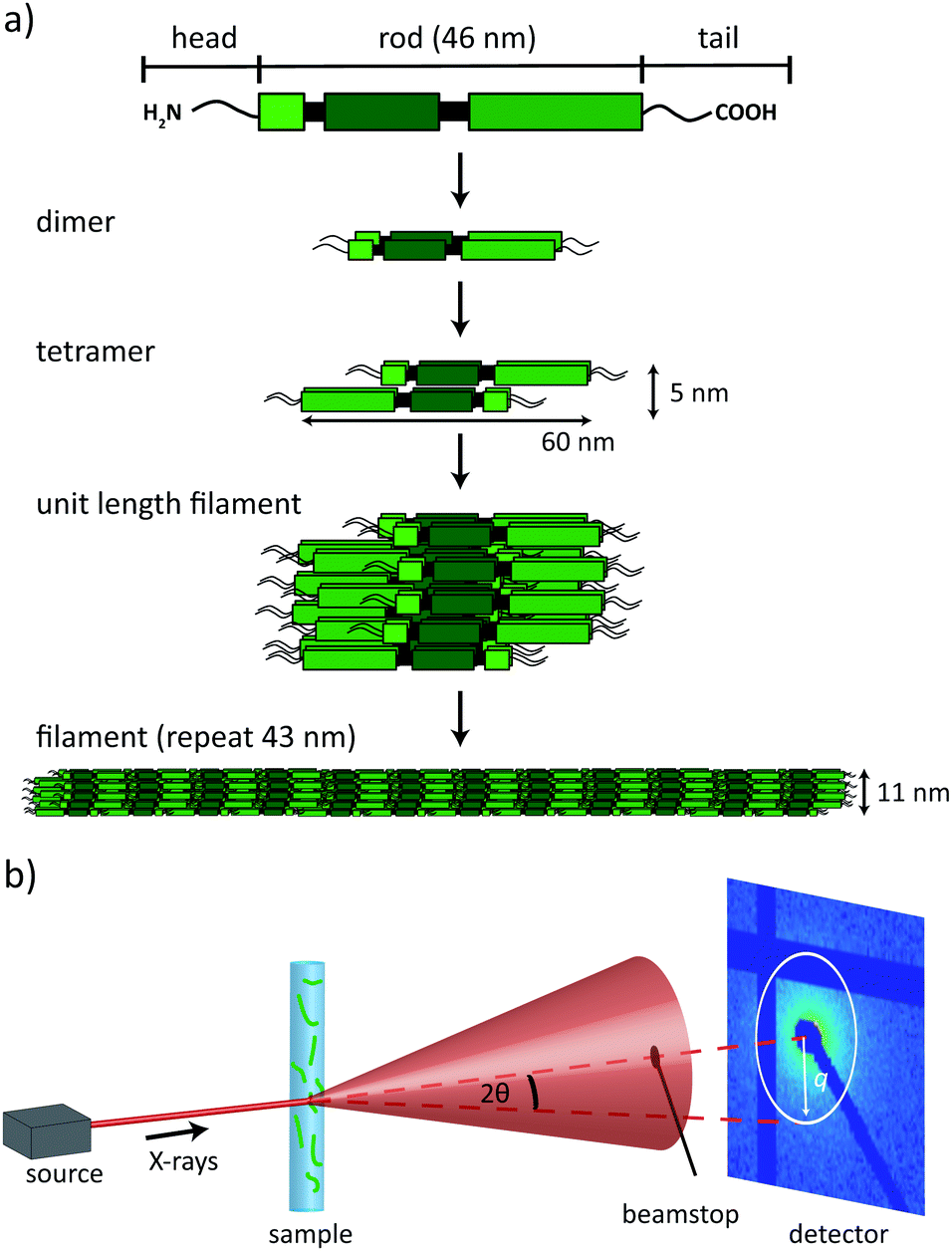

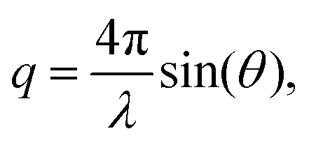
Fig. 1 (a) Schematic representation of the vimentin assembly process. Monomers consist of an α-helical rod domain, flanked by intrinsically unstructured head and tail domains. Two monomers assemble to form parallel dimers, two dimers assemble in an anti-parallel, half-staggered manner to a tetramer, and eight tetramers laterally assemble to a so-called unit length filament (ULF); lateral assembly is followed by longitudinal annealing of ULFs to extended filaments and a compaction step (sketches not to scale). (b) Schematic of the experimental setup. A capillary filled with the assembled vimentin filaments in buffer solution is placed in the X-ray beam. The primary beam is blocked by a beamstop and the scattered X-rays are recorded by a 2D pixel detector. The red dashed lines show the relation between the scattering angle 2θ and the scattering vector q⃑.

IFs are insoluble over a wide range of ionic strength, and thus, for purification they have to be denatured and kept in solution with the help of chaotropes such as urea. When renatured two monomers form parallel coiled-coils and, subsequently, anti-parallel, half-staggered tetramers that are stable in low salt buffer. Tetramers have a length of 60 nm and a diameter of 5 nm.^14,15 Upon addition of salt, tetramers laterally assemble into unit length filaments (ULFs), which – in the case of vimentin – typically consist of 32 monomers. This lateral assembly step is followed by longitudinal annealing and a compaction step, after which the filament has a diameter of 11 nm and a repeat along the filament of 43 nm. A schematic of vimentin filament assembly is shown in Fig. 1a.

According to their amino acid sequence, vimentin IFs are negatively charged. The effect of cations, especially those which also occur in the cell, on the assembly process and end state is therefore of high interest.¹⁶ Previous studies show that in vitro “standard” filaments of 32 monomers per cross-section can be initiated by addition of 160 mM NaCl or 100 mM KCl.^2,14 Small angle X-ray scattering (SAXS) reveals that the thickness of the filaments depends on the concentration of KCl present in the assembly buffer.¹⁷ Divalent ions may also be used for assembly, however, the resulting filaments display a larger, more heterogeneous diameter.^17–19 Besides the valency itself, the specific ion type has been shown to play a role for the exact assembly product. Filaments assembled in the presence of CaCl₂ are thicker and more heterogeneous compared to filaments assembled in the presence of MgCl₂.¹⁸ Vimentin filaments assembled in the presence of ZnCl₂ bundle at lower ion concentrations compared to the addition of CaCl₂.²⁰ Although these studies provide evidence that ion concentration, valency and type strongly influence vimentin assembly, systematic data are largely missing. Here, we investigate the influence of cations on the assembly of vimentin in a systematic way by combining fluorescence microscopy and SAXS. We reveal that in the presence of monovalent ions, vimentin assembles into “standard filaments” of 5 to 6 nm radius and 32 monomers per cross-section, whereas in the presence of multivalent ions, a maximum radius of 10 nm is reached, whereafter the protein forms large aggregates and precipitates.

2 Materials and methods

2.1 Protein purification, reconstitution and assembly

All chemicals are purchased from Carl-Roth GmbH (Karlsruhe, Germany) unless otherwise stated. Human wild-type (wt) vimentin, as well as vimentin C328A with additional amino acids glycine–glycine–cysteine at the C-terminus is expressed in Escherichia coli and purified from inclusion bodies as described elsewhere.^8,21 SDS-polyacrylamide gel electrophoresis is employed to control the purity of the protein. The protein is stored in 8 M urea, 5 mM tris(hydroxymethyl)aminomethane–HCl (TRIS–HCl) (pH 7.5), 1 mM ethylenediaminetetraacetic acid (ETDA), 0.1 mM ethylene glycol-bis(2-aminoethylether)-N,N,N′,N′-tetraacetic (EGTA), 1 mM 1,4-di-thiothreitol (DTT), 10 mM methylamine hydrochloride (MAC) (Merck, Munich, Germany) and roughly 0.3 M KCl at −80 °C. For the experiments, 2 mM or 20 mM 3-(N-morpholino)propanesulfonic acid–NaOH (MOPS) buffer, sodium-phosphate buffer (PB) or TRIS–HCl buffer at a pH of 7.5 are used. For reconstitution of the denatured, monomeric protein to the tetrameric form, the protein is dialyzed against urea-free buffer in a stepwise manner (6, 4, 2, 1, 0 M urea) using dialysis membranes with a 50 kDa cut-off (SpectraPor). Each dialysis step is conducted for 30 min at room temperature and the procedure is followed by an over night dialysis at 8 °C against 0 M urea, in the respective buffer. The next day, a final dialysis step against fresh buffer for 2 h at room temperature is performed. The protein concentration is determined by measuring the absorption at 280 nm (NanoDrop™, One^C, ThermoScientific Technologies, Inc., Wilmington, NC, USA). The protein is stored at 4 °C and used within one week.¹⁷

For all experiments, the “kick-start” method for assembly is employed, where the protein solution and the assembly buffer are mixed rapidly at a ratio of 1 : 1. Assembly buffer is based on 2 mM or 20 mM MOPS, PB or TRIS with twice the final salt concentration, and adjusted to pH 7.5. We employ KCl, NaCl, MgCl₂, CaCl₂, hexaaminecobalt(III) chloride (CoCl₃; Merck) and Spermine (Sp4; Merck) at various concentrations. The final protein concentration during assembly is 1 mg mL⁻¹ for SAXS experiments, 0.1 mg mL⁻¹ for atomic force microscopy (AFM) and 0.2 mg mL⁻¹ for fluorescence microscopy experiments.

For fluorescence microscopy experiments, vimentin C328A labeled with ATTO 647N (ATTO-TEC GmbH, Siegen, Germany) is mixed with wt vimentin protein prior to dialysis to enable direct visualization of the protein.^3,7,22 Usually, we add labeled vimentin up to 4%. Assembly is performed in reaction tubes for 16 h at 37 °C. The assembled filaments are diluted 1 : 100 and directly imaged with an inverted confocal microscope (FluoView IX81, Olympus Europa, Hamburg, Germany) equipped with a 60× UplanSApo oil objective (numerical aperture 1.45, Olympus). All images are obtained at room temperature.

For AFM experiments, assembly is performed for 16 h at 37 °C in reaction tubes. The protein is diluted 1 : 5 and then mixed 1 : 1 with 0.25% v/v glutaraldehyde (Polysciences Europe GmbH, Hirschberg an der Bergstrasse, Germany) for 30 s. The filaments are pipetted onto clean mica substrates (grad V5, 25 mm × 25 mm, 53-25 TED Pell, Inc., Redding, CA, USA) and incubated for 60 s. The samples are cleaned with ultra-pure water and dried with nitrogen gas. For measurements, an MFP-3D Infinity AFM (Asylum Research, Oxford Instruments, Abingdon, UK) equipped with a micro cantilever (resonant frequency of 70 kHz, spring constant 2 N m⁻¹, Olympus) is used.

For SAXS experiments assembly is performed directly in 1.5 mm diameter quartz glass capillaries, wall thickness 0.01 mm (Hilgenberg GmbH, Malsfeld, Germany) for at least 12 h at room temperature, since the solution containing assembled filaments is too viscous to be filled into the capillaries. The capillaries are sealed with wax (Hampton Research, Aliso Viejo, CA, USA) prior to the measurements.

From the comparison of vimentin assembly in the three different buffer systems (TRIS, PB and MOPS; results shown in the ESI,† including Fig. S1 and S2), we conclude that at 2 mM buffer concentration, there is no structural difference between the filaments in the three buffers used. Thus, we perform all further experiments in MOPS as a complementary approach to the more established buffer systems PB and TRIS, but with the advantage that none of the ions forms complexes with the buffer.

2.2 SAXS measurements and data treatment

SAXS measurements are performed using an in-house SAXS setup (Xeuss 2.0, Xenocs, Sassenage, France). A Genix 3D source (Xenocs) is used at a wavelength of 1.54 Å (Cu K_α radiation), 50 kV and 600 μA. Multilayer optics and scatterless slits focus the beam down to roughly 500 × 500 μm². The scattered signal is recorded at a distance of 1225 mm using a pixel detector (Pilatus3R 1M, 981 × 1043 pixels, pixel size 172 × 172 μm Dectris Ltd, Baden, Switzerland).²³ A beamstop with a size of 3 mm is placed directly in front of the detector to block the primary beam. The signal is recorded for 4 h in total for each sample, divided into 10 min intervals. In order to obtain the background signal, the same capillary is used for both the buffer measurement and the corresponding protein measurement.

For data analysis the 2D detector images are azimuthally integrated and the background is subtracted, using self-written Matlab scripts (Matlab2017a, The MathWorks, Natick, MA, USA) based on the cSAXS Matlab base package, available at https://www.psi.ch/en/sls/csaxs/software. The integrated intensity I(q) is plotted against the magnitude of the scattering vector q,

where λ is the wavelength of the radiation and 2θ is the scattering angle (Fig. 1b). SAXS data are shown in a range from 0.08 nm⁻¹ to 2.00 nm⁻¹, corresponding to real space length scales from 3.14 nm to 78 nm. At q ≈ 1.0 nm⁻¹ the signal reaches the noise level, as seen in Fig. S3 (ESI†) for a typical SAXS curve including error bars that indicate the azimuthal integration error. For clarity, we refrain from including the error bars into each of the plotted curves in Fig. 4. We study 6 ion types each at 8 concentrations. The systematic changes we observe upon changing the ion concentration (see Fig. 3) show that the statistical fluctuations of each measurement are smaller than changes due to ion concentration. To further test the statistical validity of the data, we conduct some of the measurements several times (see different shades of gray in Fig. S6–S8, ESI†) and no major differences between the data curves are observed. For each capillary, the thickness is determined using the transmission values of the empty and the water-filled capillary, prior to the actual measurement. The recorded data are normalized by the exposure time and the transmission. We furthermore correct the data by the sample thickness, i.e., the thickness of the inner diameter of the capillary at the position of the measurement. The sample thickness is calculated using the transmission scans from the empty and the water-filled capillary. The data are normalized with the correction factor (CF). The CF is needed to calculate absolute intensities in cm⁻¹ and is specific for each setup.^24,25 For our system, it is determined using water as a primary standard. In a final step, the intensities are normalized by the protein concentration.

To retrieve the radius of gyration of the cross-section R_c as well as the forward scattering I(0), the Guinier region is analyzed using the software package PRIMUS²⁶ (ATSAS, EMBL, Hamburg, Germany) as well as the open source Python library alea²⁷ using

where L is the length of the object. We fit the small q-values up to a limit of qR_c ≤ 1.3.^28,29 From I(0) we estimate the number of monomers per cross-section. R_c is defined as the root-mean-squared distance from the center of gravity of the particle:with the position vector of the ith scatterer r_i and the position vector of the center or mass r_cm. For a cylinder, as we consider it here, is smaller than the radius R. However, vimentin ULFs and filaments are better described by (partially) hollow cylinders,^30,31 for which with the inner and outer cylinder diameters R₁ and R₂, which brings R_c and the radius R closer together. Furthermore, we assume the tails of the vimentin monomers to extend from the cylindrical core,^17,32–35 which additionally increases R_c.

In addition to the Guinier analysis, we apply a model to our data that describes the vimentin filaments as monodisperse cylinders (core) surrounded by a cloud of Gaussian chains stemming from the tails of the monomers which protrude from the filament (see Fig. S4a, ESI†).^32–35 The model was first described by Pedersen³⁶ and has previously been used and thoroughly described for IF SAXS data analysis.^17,34 By construction, the model provides a lower electron density in the center of the filament, which mirrors the partial hollowness well. Briefly, the form factor of the filaments F_filament(q) can be described as

F_filament(q) = β[F_s(q) + λb²F_c(q) + 2bS_sc(q) + b²S_cc(q)], (4)

where β ∝ β_s² is the total scattering from the core per length, β_s is the forward scattering of the core per ULF, λ describes the average distance between the tails, b refers to the ratio between the scattering from the Gaussian cloud and the scattering from the core (b = β_c/β_s). The four terms define the self correlation term of the core (F_s), the self correlation of the chains (F_c) and the cross-term between the core and chains (S_sc), as well as the cross-term between different chains (S_cc). To model vimentin filaments the following assumptions are made: (i) one ULF within the filament is approximately l = 43 nm in length. (ii) The Gaussian chains are situated at the rod surface and (iii) the persistence length (1–2 μm^2,3) of the filament is larger than the accessible length scales during the measurement. The number of monomers n is set to 32 per cross-section¹⁴ and we thus obtain λ = l/n = 1.34.

In addition to the filaments in solution, we include a fraction of unassembled tetramers in the model,¹⁷ by the scattering profile of vimentin. Consequently, the form factor F_tot(q) consists of two terms

F_tot(q) = aF_filament(q) + (1 − a)I_tetramer(q) (5)

where a ∈ [0,1] is the fraction of signal arising from the filament. A more detailed description of the model is presented in the ESI.†

3 Results

3.1 Vimentin filament assembly using different ion types

In vitro assembly of vimentin filaments is typically initiated by adding monovalent ions to a vimentin tetramer solution, thus yielding μm-long smooth and flexible filaments with a diameter of about 11 nm.^2,14,17 Divalent ions such as Mg²⁺ and Ca²⁺ have also been used to initiate assembly. Notably, filaments formed are thicker and appear less flexible, compatible with a higher number of subunits per cross-section.²² However, as demonstrated by glycerol spraying/low angle rotary metal shadowing electron microscopy, they exhibit the typical 21.5 nm longitudinal repeat as seen in normal IFs and therefore keep the principal order parameters of IFs.^18,37 To systematically investigate the influence of different ions on vimentin assembly, bundling and network formation, we study five different ions, i.e., K⁺ and Na⁺ (monovalent), Mg²⁺ and Ca²⁺ (divalent), Co³⁺ (trivalent), as well as spermine, Sp₄, a polyamine that is a tetravalent polycation in solution at physiological pH. These ions all naturally occur in the cell, though at largely different concentrations. Specifically, cobalt is an essential trace element and included in B12 vitamins.³⁸ Spermine plays an important role in cellular metabolism.³⁹ In a first step, we perform fluorescence microscopy of vimentin assembled in the presence of the ions. For monovalent ions the standard concentration of 100 mM, typically used for vimentin assembly, is chosen. For the other ions, the concentrations are chosen as high as possible such that the vimentin remains in solution and does not precipitate. In the presence of monovalent ions, vimentin forms single filaments, see Fig. 2a and b. On the contrary, vimentin assembled in the presence of multivalent ions forms aggregates Fig. 2c–f. This result is in agreement with previously published work.^20,40,41 Fluorescence microscopy provides an overview of the propensity of vimentin filaments to form bundles or networks in the presence of different types of ions. The method cannot, however, shed light on the structure of the filaments formed.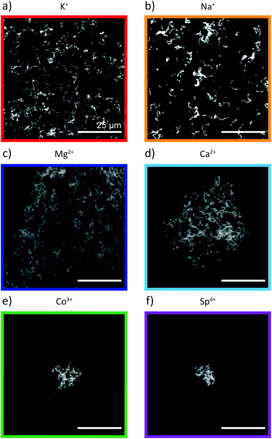

Fig. 2 Confocal fluorescence micrographs of vimentin protein assembled for 16 h; single filaments formed in the presence of (a) 100 mM KCl or (b) 100 mM NaCl; complex networks formed in the presence of multivalent ions, (c) 4 mM MgCl₂, (d) 2 mM CaCl₂, (e) 0.05 mM CoCl₃, or (f) 0.03 mM Sp₄. Visualization is achieved by including fluorescently labeled protein into the assembly system at 4%.

3.2 SAXS measurements

We complement the fluorescence microscopy experiments by SAXS measurements to gain insight into the nanoscale structure of the filaments. Here, we test eight different concentrations each, including the precipitation threshold for the multivalent ions, see Fig. 3. In each subfigure, the black data represent tetrameric vimentin, i.e., in 2 mM MOPS buffer and before initiation of assembly.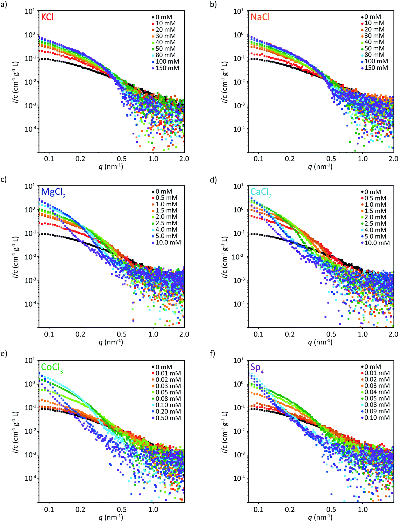

Fig. 3 Scattering data (solid circles) (the corresponding model fits are shown in Fig. S6–S8, ESI†) of vimentin assembled in the presence of eight different concentrations each of (a) KCl, (b) NaCl, (c) MgCl₂, (d) CaCl₂, (e) CoCl₃, or (f) Sp₄. The scattering profile of vimentin without additional salts is shown in black. For all multivalent ions, vimentin protein precipitates above a certain threshold ion concentration, indicated by the reduced scattering intensity.

The scattering profiles of vimentin in the presence of both monovalent ions tested here, NaCl and KCl, are almost identical over the whole concentration range, see Fig. 3a and b. With increasing ion concentration the intensity at low q-values increases, indicating that more monomers are incorporated per cross-section. Furthermore, the curves become steeper with increasing ion concentration, as consequence of an increase of the filament radius.

A similar systematic increase in intensity at low q and a steeping of the curve is observed when vimentin is assembled in the presence of multivalent ions. In contrast to the monovalent ions, however, we observe a strong change in the scattering profile after exceeding a certain threshold ion concentration, which is different for each ion, see Fig. 3c–f. The overall scattering intensity decreases, indicating precipitation of the protein. With increasing ion valency, the concentration threshold for precipitation decreases, as shown in Fig. S5 (ESI†). This observation is in agreement with previous microscopy studies of a small selection of the ions investigated here⁴¹ and can be generalized to a variety of negatively charged biopolymers.¹⁶ Interestingly, CaCl₂ shows a lower concentration threshold than MgCl₂, see Fig. 3c, d and Fig. S5 (ESI†), thus the valency of the ion is not the only determining factor for vimentin precipitation. Note that for monovalent ions, we deliberately did not increase the concentration beyond 150 mM, as with higher salt concentrations filaments start to progressively aggregate.

3.3 Structural parameters of vimentin filaments

Beyond the qualitative discussion of the SAXS curves provided in the previous section, we quantify the data in a two-fold manner. First, we analyze the Guinier region, i.e., the small q-values, of the scattering curves to retrieve the radius of gyration of the cross-section R_c as well as the forward scattering I(0), see Fig. 4. We can apply the Guinier analysis to our data, as the sample is dilute enough (1 mg mL⁻¹ protein concentration) such that there is no interaction between particles. However, for the precipitated data, this assumption is not valid and we refrain from applying eqn (2).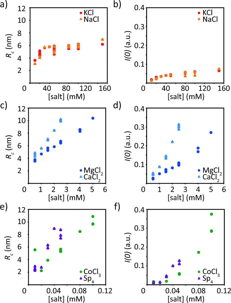

Fig. 4 Vimentin assembled in the presence of monovalent ions (KCl, NaCl, (a and b)), divalent ions (MgCl₂, CaCl₂, (c and d)), CoCl₃ and Sp₄ (e and f). Plateau reached for (a) the radius of gyration of the cross-section R_c and (b) the forward scattering I(0) at around 30 mM for both NaCl and KCl. Increase of R_c (c and e) and I(0) (d and f) for the di- and mutlivalent ions. For ion concentrations, where multiple measurements are performed, all individual data points are shown. Data from precipitated protein are not shown.

For all ions tested here, with increasing ion concentration, R_c and I(0) increase as well. However, we observe a fundamentally different behavior for mono- and divalent ions, respectively. The two monovalent ions, KCl and NaCl, influence vimentin almost in an identical manner, see Fig. 4a and b. The radius of gyration of the cross-section increases up to approximately 6 nm, which is reached at an ion concentration of 30 mM and then saturates. This is in agreement with literature, where filament radii in the range of 5–6 nm have been reported.^4,14,17,42 In parallel, we observe an increase in the forward scattering, which is a measure for the monomers per cross-section and also saturates at about 30 mM monovalent ions. When vimentin is assembled in the presence of divalent ions, a lower ion concentration is needed to initiate assembly and reach the “standard diameter” of 10 nm.^10,14 Furthermore, for divalent ions a much stronger increase in R_c and I(0) is observed (Fig. 4c and d) compared to the monovalent ions used in this study. Interestingly, the radius does not saturate as seen with monovalent ions, but increases steadily until a radius of roughly 10 nm is reached and thereafter protein precipitation occurs. Unlike the two types of monovalent ions investigated here, the two types of divalent ions differ in their effects on vimentin assembly. Vimentin assembled in the presence of CaCl₂ leads to a faster increase of both the R_c and the I(0) with concentration compared to assembly in the presence of MgCl₂. Furthermore, the concentration threshold for precipitation of vimentin assembled with CaCl₂ is lower than what we found for MgCl₂. From the increased forward scattering for divalent ions, we can estimate the maximum number of monomers per cross-section, 144 for MgCl₂ and 164 for CaCl₂ at 5 mM and 2.5 mM, respectively. These values even exceed results reported in the literature with up to twice as many monomers per cross-section for vimentin assembled in the presence of MgCl₂ as compared to monovalent ions.¹⁹ The assembly of vimentin in the presence of tri- and tetravalent ions shows a similar behavior as with divalent ions regarding the steady increase of R_c until precipitation of the protein (Fig. 4e and f). However, the ion concentrations necessary for precipitation are shifted to lower concentrations with increasing valency of the ions. The forward scattering I(0) increases as well and reaches similar values as for vimentin assembled with divalent ions, again indicating more incorporated monomers per cross-section compared to vimentin assembled with monovalent ions, i.e., 172 for CoCl₃ and 64 for Sp₄ at 0.1 and 0.05 mM, respectively.

3.4 Modeling the SAXS data

In addition to the Guinier analysis, we use a model to describe our data. This approach has the advantage that not only the low q-values are taken into account, but the whole accessible data range is considered. In the model, we include a solid cylindrical core decorated by a cloud of Gaussian chains, as schematically shown in Fig. S4 (ESI†). All data fits are shown in Fig. S6–S8 (ESI†). The fits match the corresponding data well. Note that the tetrameric scattering profile (black in Fig. 3) is not fitted, as the model does not apply to the tetrameric state of vimentin. The fit leads to quantitative values for the radius of the filament core and the contribution of the tetrameric pool to the scattering profile, see Fig. 5.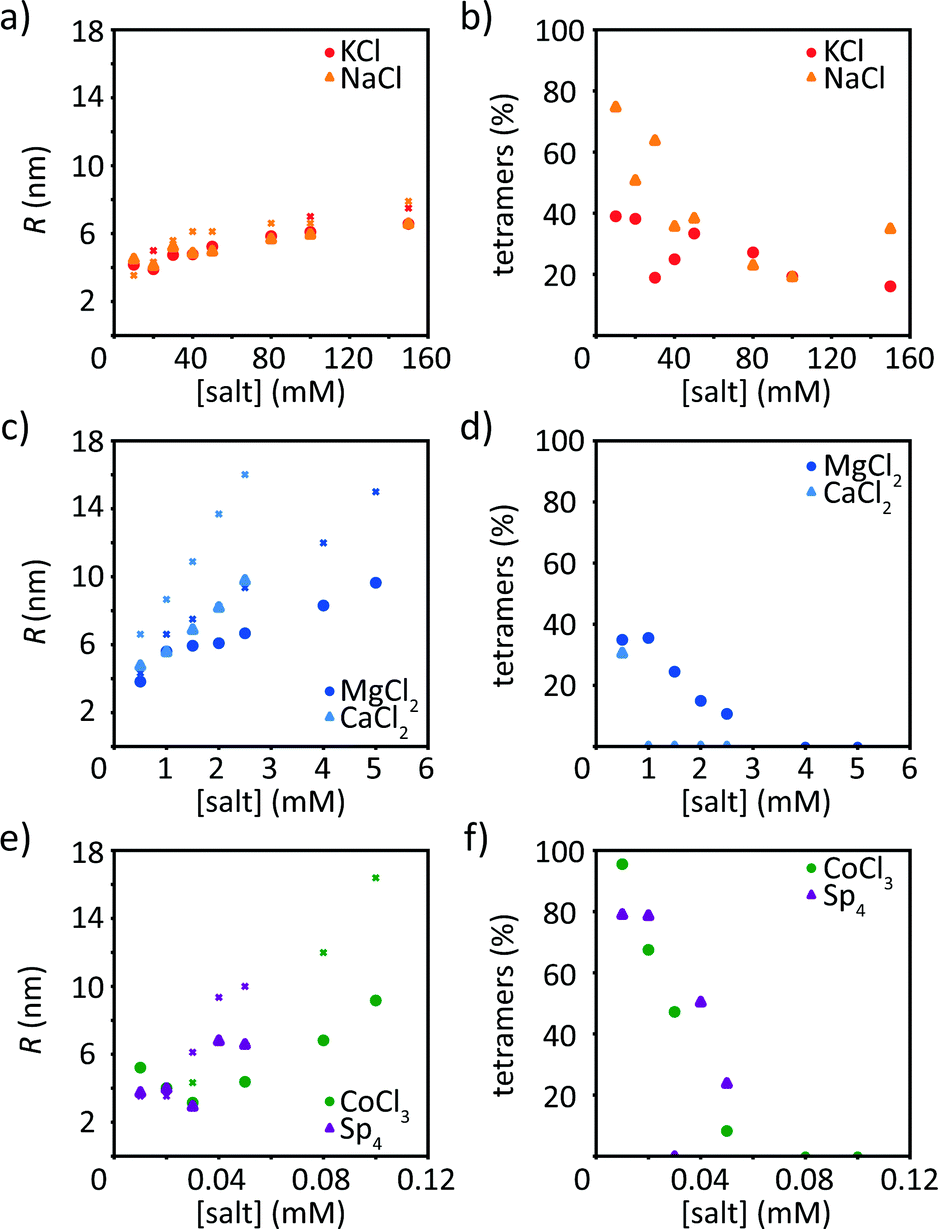

Fig. 5 Results of the model fit (see schematic in Fig. S4, ESI†) for monovalent ions (KCl, NaCl, (a and b)), divalent ions (MgCl₂, CaCl₂, (c and d)), CoCl₃ and Sp₄ (e and f). (a, c and e) Filament radius R. For comparison, the crosses show the calculated radii at each concentration based on the number of monomers retrieved from the Guinier analysis and a radius of 2.5 nm for a tetramer. (b, d and f). Amount of tetramers remaining in solution after assembly. Data from precipitated protein are not shown.

As a result of these fits, we observe that for all ion types the radius of the filament R increases with increasing ion concentration. This is expected and in agreement with the Guinier analysis. Furthermore, the contribution of the tetramers decreases with increasing ion concentration, indicating that more tetramers are incorporated in the filament (Fig. 5b, d and f). Interestingly, for CaCl₂ there is a measurable tetrameric contribution only at the lowest ion concentration. The parameter a (see eqn (5)) indicates the distribution to the scattering stemming from the filaments and not the respective protein mass. It is therefore not straight forward to provide a quantitative relation between the scattering power of tetramers remaining in solution and I(0). Fig. S9 (ESI†) shows that, as expected, I(0) decays with the percentage of scattering intensity stemming from tetramers, and it decays faster than linearly, which is due to the fact that larger scatters contribute more strongly to the intensity than smaller ones (i.e. tetramers). The filament radii are similar to the results of the Guinier analysis, including all trends described above. Interestingly, the radii for vimentin in the presence of trivalent CoCl₃ or tetravalent Sp₄ are slightly smaller than the corresponding R_c from the Guinier analysis. The decrease in radius at low concentrations may be due to different tetramer pools. Apart from the filament radii, the radii of gyration of the disordered tail domains, R_g, which decorate the surface of the cylindrical filament core, are obtained from the fits. Fig. S4b (ESI†) schematically shows the radial electron density distribution of the modeled filament. As a general trend, R_g increases with increasing ion concentration, which we attribute to a swelling of the Gaussian chains. Interestingly, the swelling process occurs already at lower ion concentrations for high valency, in agreement with the precipitation threshold for the different ion types, see Fig. S10 (ESI†). Thus, our observation could be linked to the ability of the tails to mediate cross-linking of filaments in the presence of di- or multivalent ions.⁴⁰

An additional comparison of the two data analysis methods is performed by calculating a “theoretical filament diameter” from the number of monomers as retrieved by the Guinier analysis and a diameter of 5 nm for a tetramer,^14,15 shown as crosses in Fig. 5a, c and e. The theoretical value agrees well with the data for vimentin assembled with monovalent ions, but not for multivalent ions. The theoretical diameter exceeds R_c from the Guinier analysis by about 10–20% for monovalent ions and 30–40% for multivalent ions. One reason for the difference could be the compaction step, which reduces the thickness of the filament but the number of monomers stays equal. Another reason could be a more compact structure because of electrostatic interactions.

3.5 The influence of the ion valency

To render our results more comparable between different ion types, we plot R_c against the ionic strength, see Fig. 6a. As described above, for monovalent ions the radius of gyration of the cross-section increases to roughly 6 nm at an ionic strength of 30 mM and then saturates. All multivalent ions lead to similar results, albeit strikingly different from the monovalent ions. The corresponding data all collapse on one curve, no saturation of the radius is observed and they all reach a radius of roughly 10 nm at an ionic strength around 5–15 mM, before precipitation occurs. This supports our impression from microscopy, that monovalent ions do not initiate precipitation in the measured range but saturate at a constant radius and an increase in the ionic strength does not change the radius much, which is in stark contrast to multivalent ions. When plotting the forward scattering I(0) against R_c, see Fig. 6b, we observe that the data for low ion concentrations collapse on one curve. This indicates that at a given radius, the filaments have a similar number of monomers per cross-section, regardless of the ion type and concentration used for assembly. The “standard filament” consists of 32 monomers per cross-section, which is indicated by the dashed horizontal line in Fig. 6b. This value is exceeded by vimentin assembled in the presence of multivalent ions, as discussed above. By calculating a theoretical curve, where the I(0) value at 100 mM KCl corresponds to 32 monomers (8 tetramers) we determine the theoretical radius for a cylinder with a radius of 2.5 nm per tetramer, as shown by the crosses in Fig. 6b. Note that this estimate is performed assuming filled cylinders, although there is evidence of partial hollowness.³⁰ At low ion concentrations, the theoretical curve fits the data well, whereas at higher ion concentrations, more monomers per cross-section are present as compared to the theoretical curve.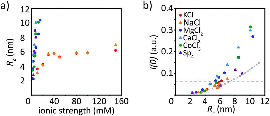

Fig. 6 (a) The radius of gyration as obtained from the Guinier analysis plotted against the ionic strength, for all ions investigated here (for color code, see b). (b) Increase of I(0) with increasing R_c. The dashed line indicates I(0) for a “standard filament” with 32 monomers (assembled at 100 mM KCl). They gray crosses refer to the theoretical curve based on a radius of 2.5 nm for a tetramer and that at 100 mM KCl the I(0) value corresponds to 32 monomers.

4 Discussion

From our systematic study of vimentin assembly in the presence of different ion types and concentrations, we can draw several general conclusions. First, the higher the valency of the ion, the lower the concentration needed to induce assembly or precipitation, i.e., roughly one order of magnitude per charge of the ion, in agreement with the suggestion in ref. 41. Secondly, there seems to be a principle difference between the behavior of vimentin in the presence of monovalent ions compared to vimentin in the presence of multivalent ions. For monovalent ions, the radius of gyration of the cross-section R_c, the filament radius R and the forward scattering I(0) reach a plateau at 30 mM, whereas for multivalent ions, no plateau is found but R increases up to 10 nm, thus about twice the “typical” radius for filaments assembled in monovalent salt, until precipitation of the protein occurs. Consequently, the number of monomers saturates at roughly 32 per cross-section when the assembly is induced by monovalent ions. For multivalent ions, we find up to 172 monomers per cross-section with increasing ion concentration until the protein precipitates i.e. it assembles into very dense, insoluble networks. This is in agreement with the literature, where Herrmann et al. found filaments with up to two or three times more monomers per cross-section when vimentin is assembled in the presence of MgCl₂.¹⁹ In particular, we show that vimentin forms single filaments in the presence of monovalent ions and networks in the presence of multivalent ions. A reason for the different behavior in single filament versus network formation could be found in differing lateral interactions between vimentin subunits. For monovalent ions, the negatively charged groups of the vimentin amino acid sequence are screened by the positive counterions leading to less repulsion and the assembly is facilitated. For multivalent ions, by contrast, counterion condensation is expected. Thus, counterions bridge to other negative charges of other monomers within the same or different filaments and induce attraction. These strong forces could lead to network or aggregate formation.

Interestingly, we observe a difference between the two divalent ions, CaCl₂ and MgCl₂, regarding the concentration needed for precipitation, supporting earlier reports.^18,20 This phenomenon can be explained by the Hofmeister effect that puts cations in an order according to their ability to precipitate proteins.^43–46 Looking at the Hofmeister series for the ions used here, we obtain K⁺ > Na⁺ > Mg²⁺ > Ca²⁺, matching our findings. For our system, we are able to extend the Hofmeister series by Co³⁺. By contrast, it is not straightforward to draw conclusions on the effect of ion size, as this parameter does not systematically influence our results.

Due to the size, the ions also have different ionization energies. Ca²⁺ has a lower ionization energy than Mg²⁺ and thus the two electrons in the outer shell can more easily interact with the charges of vimentin. Comparing all vimentin radii with respect to the ionic strength, the data collapse and the protein precipitation threshold is on the order of 10 mM, i.e., 15 mM for MgCl₂, 5–7.5 mM for CaCl₂ and CoCl₃ and 5 mM for Sp₄. This indicates that multivalent ions have the same effect on vimentin assembly, regardless of their valency.

5 Conclusions

To conclude, we provide insights into the assembly mechanism of vimentin, and possibly IFs in general, although differences in the charge pattern due to differences in the amino acid sequence may play an important role. Whereas monovalent ions lead to the ordered assembly of vimentin into “standard filament” incorporating 32 monomers per ULF during lateral assembly, for multivalent ions this lateral assembly step allows for a denser packing of subunits by enhancing more ordered interactions of the negatively charged rods due to their ability to introduce stable cross-links. The results could potentially be relevant in the cell, as local ion concentrations can be expected to differ considerably from average intracellular concentrations.

Conflicts of interest

There are no conflicts to declare.

Acknowledgements

We thank Susanne Bauch for technical support and Norbert Mücke for fruitful discussions. We furthermore thank Andreas Janshoff and his group, as well as Anna Schepers and Julia Kraxner for support with the AFM measurements. This work was financially supported by the Deutsche Forschungsgemeinschaft (DFG, German Research Foundation) in the framework of the SFB 755, “Nanoscale Photonic Imaging”, project B07, and the SFB 860, “Integrative Structural Biology of Dynamic Macromolecular Assemblies”, project B10. Furthermore the work was supported by the Deutsche Forschungsgemeinschaft (DFG, German Research Foundation) under Germanys Excellence Strategy – EXC 2067/1-390729940. M. M. was supported by the Weierstrass Institute for Applied Analysis and Stochastics.

References

1. F. Huber, A. Boire, M. P. López and G. H. Koenderink, Curr. Opin. Cell Biol., 2015, 32, 39–47.
2. N. Mücke, T. Wedig, A. Bürer, L. N. Marekov, P. M. Steinert, J. Langowski, U. Aebi and H. Herrmann, J. Mol. Biol., 2004, 340, 97–114.
3. B. Nöding, H. Herrmann and S. Köster, Biophys. J., 2014, 107, 2923–2931.
4. L. Kreplak and D. Fudge, BioEssays, 2006, 29, 26–35.
5. Z. Qin, L. Kreplak and M. J. Buehler, PLoS One, 2009, 4, e7294.
6. Z. Qin, L. Kreplak and M. J. Buehler, Nanotechnology, 2009, 20, 425101.
7. J. Block, H. Witt, A. Candelli, E. J. Peterman, G. J. Wuite, A. Janshoff and S. Köster, Phys. Rev. Lett., 2017, 118, 048101.
8. J. Block, H. Witt, A. Candelli, J. C. Danes, E. J. G. Peterman, G. J. L. Wuite, A. Janshoff and S. Köster, Sci. Adv., 2018, 4, eaat1161.
9. J. Forsting, J. Kraxner, H. Witt, A. Janshoff and S. Köster, Nano Lett., 2019, 19, 7349–7356.
10. E. Fuchs and K. Weber, Annu. Rev. Biochem., 1994, 63, 345–382.
11. I. Szeverenyi, A. J. Cassidy, C. W. Chung, B. T. Lee, J. E. Common, S. C. Ogg, H. Chen, S. Y. Sim, W. L. Goh, K. W. Ng, J. A. Simpson, L. L. Chee, G. H. Eng, B. Li, D. P. Lunny, D. Chuon, A. Venkatesh, K. H. Khoo, W. I. McLean, Y. P. Lim and E. B. Lane, Hum. Mutat., 2008, 29, 351–360.
12. H. Herrmann, S. V. Strelkov, P. Burkhard and U. Aebi, J. Clin. Invest., 2009, 119, 1772–1783.
13. A. A. Chernyatina, D. Guzenko and S. V. Strelkov, Curr. Opin. Cell Biol., 2015, 32, 65–72.
14. H. Herrmann, M. Häner, M. Brettel, S. A. Müller, K. N. Goldie, B. Fedtke, A. Lustig, W. W. Franke and U. Aebi, J. Mol. Biol., 1996, 264, 933–953.
15. A. A. Chernyatina, S. Nicolet, U. Aebi, H. Herrmann and S. V. Strelkov, Proc. Natl. Acad. Sci. U. S. A., 2012, 109, 13620–13625.
16. P. A. Janmey, D. R. Slochower, Y.-H. Wang, Q. Wen and A. Cēbers, Soft Matter, 2014, 10, 1439.
17. M. E. Brennich, S. Bauch, U. Vainio, T. Wedig, H. Herrmann and S. Köster, Soft Matter, 2014, 10, 2059–2068.
18. I. Hofmann, H. Herrmann and W. W. Franke, Eur. J. Cell Biol., 1991, 56, 328–341.
19. H. Herrmann, M. Häner, M. Brettel, N.-O. Ku and U. Aebi, J. Mol. Biol., 1999, 286, 1403–1420.
20. H. Wu, Y. Shen, D. Wang, H. Herrmann, R. D. Goldman and D. A. Weitz, Biophys. J., 2020, 119, 55–64.
21. H. Herrmann, L. Kreplak and U. Aebi, Intermediate Filament Cytoskeleton, Elsevier, 2004, pp. 3–24.
22. S. Winheim, A. R. Hieb, M. Silbermann, E.-M. Surmann, T. Wedig, H. Herrmann, J. Langowski and N. Mücke, PLoS One, 2011, 6, e19202.
23. B. Henrich, A. Bergamaschi, C. Broennimann, R. Dinapoli, E. Eikenberry, I. Johnson, M. Kobas, P. Kraft, A. Mozzanica and B. Schmitt, Nucl. Instrum. Methods Phys. Res., Sect. A, 2009, 607, 247–249.
24. C. A. Dreiss, K. S. Jack and A. P. Parker, J. Appl. Crystallogr., 2006, 39, 32–38.
25. L. Fan, M. Degen, S. Bendle, N. Grupido and J. Ilavsky, J. Phys.: Conf. Ser., 2010, 247, 012005.
26. P. V. Konarev, V. V. Volkov, A. V. Sokolova, M. H. J. Koch and D. I. Svergun, J. Appl. Crystallogr., 2003, 36, 1277–1282.
27. M. Eigel, R. Gruhlke, M. Marschall, P. Trunschke and E. Zander, alea – A Python Framework for Spectral Methods and Low-Rank Approximations in Uncertainty Quantification, https://bitbucket.org/aleadev/alea.
28. D. I. Svergun and M. H. J. Koch, Rep. Prog. Phys., 2003, 66, 1735–1782.
29. H. D. Mertens and D. I. Svergun, J. Struct. Biol., 2010, 172, 128–141.
30. D. A. Parry, S. V. Strelkov, P. Burkhard, U. Aebi and H. Herrmann, Exp. Cell Res., 2007, 313, 2204–2216.
31. K. N. Goldie, T. Wedig, A. K. Mitra, U. Aebi, H. Herrmann and A. Hoenger, J. Struct. Biol., 2007, 158, 378–385.
32. S. V. Strelkov, J. Schumacher, P. Burkhard, U. Aebi and H. Herrmann, J. Mol. Biol., 2004, 343, 1067–1080.
33. M. Kornreich, R. Avinery, E. Malka-Gibor, A. Laser-Azogui and R. Beck, FEBS Lett., 2015, 589, 2464–2476.
34. C. Y. J. Hémonnot, M. Mauermann, H. Herrmann and S. Köster, Biomacromolecules, 2015, 16, 3313–3321.
35. H. Herrmann and U. Aebi, Cold Spring Harbor Perspect. Biol., 2016, 8, a018242.
36. J. S. Pedersen, J. Appl. Crystallogr., 2000, 33, 637–640.
37. D. Henderson, N. Geisler and K. Weber, J. Mol. Biol., 1982, 155, 173–176.
38. K. Czarnek, S. Terpiłowska and A. K. Siwicki, Cent. Eur. J. Immunol., 2015, 2, 236–242.
39. W. Yuan and H. Li, Nanostructures for Drug Delivery, Elsevier, 2017, pp. 445–460.
40. Y.-C. Lin, N. Y. Yao, C. P. Broedersz, H. Herrmann, F. C. MacKintosh and D. A. Weitz, Phys. Rev. Lett., 2010, 104, 058101.
41. C. Dammann, H. Herrmann and S. Köster, Isr. J. Chem., 2015, 56, 614–621.
42. U. Aebi, M. Häner, J. Troncoso, R. Eichner and A. Engel, Protoplasma, 1988, 145, 73–81.
43. F. Hofmeister, Arch. Exp. Pathol. Pharmakol., 1888, 24, 247–260.
44. A. Salis and B. W. Ninham, Chem. Soc. Rev., 2014, 43, 7358–7377.
45. R. Baldwin, Biophys. J., 1996, 71, 2056–2063.
46. H. I. Okur, J. Hladílková, K. B. Rembert, Y. Cho, J. Heyda, J. Dzubiella, P. S. Cremer and P. Jungwirth, J. Phys. Chem. B, 2017, 121, 1997–2014.

---

Footnote

† Electronic supplementary information (ESI) available: Comparison of different buffer systems; azimuthal integration error; detailed description of the theoretical model; precipitation thresholds; additional data plots. See DOI: 10.1039/d0sm01659d

---