Supercritical water gasification of wet biomass residues from farming and food production practices: lab-scale experiments and comparison of different modelling approaches

Abstract

Globally, large amounts of biomass wastes such as cattle manure, fruit/vegetable waste, and cheese whey residual streams are disposed of from farming and food processing industries. A promising approach to convert such biogenic residues into valuable biofuels is Supercritical Water Gasification (SCWG). A detailed investigation on SCWG of the mentioned wet biomass wastes has been performed to assess the thermodynamic behavior of such a complicated system. This is conducted by combining advanced models with a supplementary experimental study, providing deep insight into the behavior of the SCWG system for different bio-waste sources. For the modelling part, different approaches including global, constrained and thermal quasi-thermodynamic equilibria have been pursued to analyze the influence of operating parameters on the produced biogas quality. Furthermore, SCWG experiments were conducted using biomass samples provided by our industrial partner. Reasonable agreements were observed between experimental results and predictions from constrained and thermal-quasi equilibrium models, showing significant improvements over the global thermodynamic equilibrium model. Results showed that superimposition of carbon conversion efficiency together with the use of a constant molar amount of specific compounds can improve the accuracy of the global equilibrium model. Furthermore, comparisons between different models revealed the advantage of the thermal quasi-equilibrium model, which uses the “approach temperature” concept, over the constrained equilibrium model, by reducing the complexities inherent in superimposing multiple constraints. Overall, the thermal-quasi equilibrium approach has its advantages of lumping all the additional constraints used in the constrained equilibrium model into an effective approach temperature, offering (i) a better reproducibility of the experimental data point and (ii) a rigorous basis for scale-up calculation. The results of this study provide a better understanding of the SCWG process for different types of wet biomass feedstocks as result of applying advanced analytical approaches and comparing with experiments.

---

Introduction

Global energy overview

Despite that renewable energy sources have been growing at an inspiring rate and have outpaced the growth of other sources of energy, global energy conversion systems continue to be dependent mainly on fossil fuels. According to the International Energy Agency (IEA), natural gas, coal, and oil still constitute 81% of the 599.34 EJ world's total primary energy demand.¹ It has been anticipated that under the “current policies” scenario of the IEA, the primary energy demand will steadily increase, reaching 19 177 MTOE by 2040.¹ However, currently, fossil fuels are facing the challenge of depletion. In addition, according to the IEA, an immense increase in CO₂ emissions caused by the use of fossil fuels, say from 23.1 to 33.2 Gt between 2000 and 2018 with the expectation of reaching 41.3 Gt by 2040,¹ poses a major environmental threat to the planet. Having assessed the prevailing challenges associated with the depletion of fossil fuel reserves, global increase of energy demand and emission problems, it is crucial to accelerate the process of transition to a renewable energy-based economy.

Globally, biomass-based energy supply forms the largest renewable energy source with a total primary energy supply of 56.5 EJ in 2016, thus constituting 70% share among all the renewable energy sources.² In fact, bioenergy is derived from different resources such as wood, crop residues, forestry residues, municipal and industrial wastes, energy crops, algae, and animal manure, to name a few. In principle, the first-generation biomass includes food crops such as wheat, corn, and sugarcane and pose challenges related to food vs. fuel competition. Such challenges were overcome by developing the second biomass generation which comprises wood, grass, and food crop waste including straw, organic waste, etc. The third generation of biomass mainly includes algae which are specially engineered energy crops. Among all, both industrial and municipal wastes, which form part of the second-generation biomass, have gained prominence, as the environmental issues have become significantly recognized over the last decade. For instance, it is reported that the waste energy sector contributed 2.17 EJ of energy globally.² A few of the wet waste streams such as fruit/vegetable waste, cattle manure, and cheese whey form a substantial part of the second-generation biomass and are gaining importance. This is due to their massive quantities, and energy recovery from such waste sources can locally contribute to solving the prevailing environmental and energy supply problems in the areas of agricultural and food processing. According to the FAO and WEF, nearly 1.3 billion tons of food produced for human consumption are wasted around the world every year, which comprises 45 wt% fruits and vegetables.^3,4 The carbon footprint from such quantities of food wastage is around 4.4 Gt CO₂ equivalent per year, including land-use change.⁵ Furthermore, in general, 29.7 billion livestock animals produce approximately 3.1 Gt of feces every year,⁶ of which cattle, among the largest animal population (nearly 1.5 billion), produce an average of 1.3 Gt feces. Cheese whey as a liquid by-product is produced after the precipitation of milk during the cheese production process. Basically, the chemical oxygen demand (COD) and biochemical oxygen demand (BOD) in whey can vary between 50 000 and 80 000 mg L⁻¹ and 40 000 to 60 000 mg L⁻¹, respectively, resulting in soil depletion upon disposal,⁷viz. high COD and BOD values lead to rapid consumption of oxygen content of soil due to the breakdown of sugars and proteins. According to the available reports, around 90 vol% of the feed to a cheese production line is converted to whey, resulting in the annual production of 21.6 million tons of cheese whey globally.⁸ Such potential sources of energy are among the most appealing sources concerned with sustainable development. These potential sources can be converted into useful energy forms through either thermochemical or biochemical conversion routes (after pretreatment), e.g., combustion, gasification, liquefaction, pyrolysis, digestion and fermentation. Among these process routes, gasification is merited to be one of the most preferred and possible processes as even the converted biomass can be utilized in different energy supply markets such as transportation, electricity, and heat.⁹ However, the use of conventional gasifiers for the conversion of biomass feedstocks with more than 75% MC is not feasible without pretreatment stages such as drying.¹⁰

Basically, biomass has a higher moisture content than fossil fuels like coal. However, wet waste streams such as fruit/vegetable waste, cattle manure and cheese whey have an even higher moisture content, which can exceed 90 wt% on as-received basis.¹⁰ Higher moisture content results in a negative impact on gasification efficiencies as extra energy (approximately 2242 kJ per kg-moisture) is consumed in water evaporation.¹⁰ Furthermore, experimental studies demonstrate that the total thermal efficiency‡ in the gasification process is inversely proportional to water content, e.g. the total efficiency‡ diminishes approximately from 60% to 25% when the water content in the feed increases from 5 to 75%.¹¹ An alternative option to conventional biomass gasification and anaerobic digestion is SCWG. Among others, SCWG offers a major advantage as this process is not basically pertinent to dry biomass compared with conventional gasification. However, for very high moisture content residue streams, say higher than 90%, the feedstock should undergo a dewatering stage before SCWG, as the initial moisture content plays a significant role in the thermal efficiency of the system.¹⁰ Furthermore, the SCWG process offers a much shorter residence time in the reactor ranging from a few seconds to a few minutes than anaerobic digestion of wet biomass where the residence time is in the order of days.¹²

Even though SCWG is a promising technology for wet biomass processing, it still faces commercialization issues due to some technical and practical impediments such as large heat input requirements for the endothermic reactions. Such a large heat demand affects the thermal energy efficiency of the SCWG process and thus imposes high capital cost, as it should be either supplied from outsourced heating media or recovered from the gas product stream, entailing highly efficient heat exchangers.¹⁰ Furthermore, feeding large quantities of wet biomass, which is intrinsically fibrous and heterogeneous, requires a high-capacity slurry pump, thus incurring high capital cost.^10,13 There are also some operational challenges associated with the SCWG process such as the possibility of plugging in the biomass preheater due mainly to char and tar formation in the tube side¹⁴ and in the reactor, which stems from the low solubility of salts in the SCW.¹⁵

In principle, SCWG takes place in a dense fluid phase under supercritical water conditions, i.e., with temperature and pressure above 374.29 °C and 221 bar, respectively. The gasification can be classified into two temperature regimes, near-critical temperature conversion (375–500 °C) in the presence of a catalyst and high-temperature (>500 °C) non-catalytic processing.¹⁰ Back in the 1970s, supercritical water (SCW) was first explored as a gasifying medium with organic material being gasified under supercritical conditions. Modell et al.^17,18 filed a patent to report the gasification of organic materials, including maple sawdust, glucose, and sewage sludge, to name a few. Since then, SCWG of high moisture content biomass has been the subject of numerous analytical and experimental research studies.^{11,15–17,19–25} The current status of research in this field is discussed hereinafter, by providing a detailed literature survey.

Experimental overview

Nanda et al.^16,26 conducted experimental studies on SCWG of several agricultural residues and fruit wastes including banana, orange, pineapple, and lemon peel, coconut shell, sugarcane bagasse and aloe vera rind in a tubular batch reactor (length: 10 in., outer diameter: 0.5 in. and inner diameter: 0.37 in.). The authors investigated the influences of different parameters such as temperature (400–600 °C), pressure (230–250 bar), reaction time (15–45 min) and catalyst (NaOH and K₂CO₃) on the gasification behaviour. In the case of orange peel as the feed, the optimal conditions for total gas and hydrogen yields were reported as 600 °C (temperature), 230–250 bar (pressure), 45 min (residence time), and 1 : 10 (biomass-to-water ratio), which give a high LHV of 722 kJ N m⁻³ for the syngas produced. Furthermore, the authors assessed the use of fructose as a model compound for fruit/vegetable waste using different parameters. For the case of fructose as the feedstock, the optimal conditions for total gas yield, hydrogen yield and carbon gasification efficiency (CGE) were found to be 700 °C (temperature), 250 bar (pressure), 4 wt% (feed), and 60 s (residence time) while the highest LHV for syngas production was reported as 3630 kJ m⁻³ by using 0.8 wt% KOH as the catalyst. The authors concluded that temperature plays an essential role in the gasification of food wastes, as their results show that the gas yield (H₂, CH₄, and CO₂) and CGE increase upon increasing the temperature. In another study, Amrullah and Matsumara²⁷ investigated phosphorus recovery and gas generation from sewage sludge in a continuous SCWG tubular reactor. Experiments were conducted in the temperature range of 500–600 °C, at a pressure of 250 bar, a feedstock flow rate of 1.3–15 mL min⁻¹ and a residence time of 5–60 s. Furthermore, the authors developed a first order reaction kinetics model showing a satisfactory agreement with the experimental results. They observed that during the reaction, the organic phosphorus content is quickly converted to inorganic phosphorus, with a residence time of 10 s. The authors also observed a CGE of 73% at a temperature of around 600 °C. The SCWG of municipal waste leachate followed by catalytic gas upgradation was investigated by Molino et al.²⁸ The gasification tests were conducted in a continuous tubular reactor with the flow rate within the range of 10–40 mL min⁻¹, a process time of 20–60 min and at a temperature and pressure of 550 °C and 250 bar, respectively. The produced syngas was then upgraded to increase the methane fraction of synthetic natural gas using a Ni-based catalyst. The authors showed that a two-stage process including SCWG of waste followed by catalytic upgrading produces syngas with a calorific value of 15–17 MJ kg⁻¹. Furthermore, the authors reported that methane concentration in syngas increased by 50 v/v% with the assistance of the Ni catalyst. Chen et al.²⁹ investigated the supercritical gasification of sewage sludge in a fluidized bed reactor in a detailed experimental study, wherein the effects of different operating parameters such as feedstock concentration, temperature, alkali catalysts and their loading on gaseous products and carbon distribution are investigated. The authors performed multiple experiments using sewage sludge with a concentration of 4–12 wt%, in the temperature range of 480–540 °C and under a pressure of 250 bar. The results of this study showed that the CGE increases with the increase in temperature, and the use of an alkali catalyst can enhance the hydrogen production. Table 1 gives an overview of the experiments conducted in recent past using real wet biomass feedstocks.

Table 1 Overview of some of the experimental studies conducted in the past using real biomass feedstocks

Author(s) (year)	Biomass type	Operating conditions							Yield
		Reactor type	Temperature (°C)	Pressure (bar)	Res. time (s)	Feed conc. (wt%)	Flow rate (mL min^−1)	CGE (%)	H2	CO2	CH4	CO
Nanda et al.^16,26 (2015)	Fructose	Continuous flow	700	250	60	4	NA	88	3.3 mol mol^−1 feed	3.2 mol mol^−1 feed	1.2 mol mol^−1 feed	0.2 mol mol^−1 feed
Nanda et al.^24 (2015)	Orange peel	Batch type	600	230–250	2700	10	Na	14.8	1.6 mmol g^−1 feed	3.3 mmol g^−1 feed	1.4 mmol g^−1 feed	0.25 mmol g^−1 feed
Amrullah and Matsumara^27 (2017)	Sewage sludge	Continuous flow	600	250	60	NA	1.3–15	73	20 vol%	25 vol%	40 vol%	NA
Molino et al.^28 (2017)	Municipal waste leachate	Continuous flow	550	250	1200	NA	40	6	25 vol%	45 vol%	18 vol%	12 vol%
Chen et al.^29 (2013)	Sewage sludge	Continuous flow	480–540	250	NA	4	150 g min^−1	35–45	6.5–9 mol kg^−1	8–9 mol kg^−1	1–2.5 mol kg^−1	0.5–0.1 mol kg^−1

---

Thermodynamic equilibrium modeling overview

Thermodynamic equilibrium modeling was first employed by Antal et al.²² to assess the gasification behavior of different biomass feedstocks, e.g. potato waste, potato and corn starch gel and wood saw in a cornstarch gel. The researchers conducted experiments at temperatures and pressures above 650 °C and 220 bar, respectively. The test results were then compared to the equilibrium concentrations predicted by STANJAN and HYSIM. Basically, STANJAN uses the ideal gas law as an equation of state (EOS) and the Peng–Robinson EOS is employed for HYSIM. The results of different test campaigns in this study showed (i) no tar product, (ii) low COD (49–54 mg L⁻¹) and total organic carbon, TOC (0.3–0.5 wt% carbon content in feed) with a pH between 3 and 8 for the liquid effluent. Following this, several research groups put the basis of their analytical study on thermodynamic equilibrium modelling. Tang and Kitagawa³⁰ developed a thermodynamic model based on Gibbs free energy minimization to estimate the product gas composition for supercritical gasification of biomass. The authors used the Peng–Robinson EOS in their modeling to investigate SCWG of methanol, glucose, cellulose, starch, and sawdust. One of their interesting observations was a very limited effect of pressure on the yield of gases. Yanagida et al.³¹ used the thermodynamic equilibrium modeling approach for SCWG of poultry manure. The authors used HSC Chemistry 6.12 software to predict the equilibrium composition of both organic and inorganic elements including carbon, hydrogen, oxygen, calcium, sodium, potassium, chlorine, silicon, sulfur, and phosphorus. The equilibrium compositions were compared with the experimental results conducted at 600 °C and 320 bar along with activated carbon as the catalyst. The authors observed that most of the silicon, calcium and phosphorus are found in the solid phase whereas almost all of chlorine, sodium and potassium appear in the liquid phase during SCWG of the biomass. Yakaboylu et al.^9,25,32–35 employed different approaches to model the thermochemical conversion in a supercritical water gasifier. The authors developed unconstrained and constrained equilibrium models to assess the behavior of gaseous products together with the distribution of elements under different gasification conditions for different feedstocks including cattle manure. The researchers concluded that the accuracy of the models can be increased with the use of constrained equilibrium modeling. The authors also found that CGE is the most important additional constraint to improve the GTE model. Lu et al.¹⁴ conducted a comprehensive thermodynamic analysis on supercritical gasification of wood sawdust. Furthermore, the authors studied the chemical equilibrium in a reactor, gas–liquid equilibrium in a high-pressure separator and exergy and energy analyses of the entire system. The analysis of chemical equilibrium demonstrated that hydrogen production increases with the increase of temperature. According to this study, the gas–liquid equilibrium analysis showed that an increase in pressure and temperature in the high-pressure separator assisted in the purity of hydrogen in the gas phase but hindered the hydrogen recovery ratio. Table 2 gives an overview of the global thermodynamic equilibrium (GTE) modeling approaches for SCWG of biomass studied in the past.

Table 2 Overview of some of the research studies conducted using GTE modeling approaches for SCWG of biomass feedstocks

Author(s) (year)	Biomass type	EoS/software used	Phases considered
Antal et al.^22 (2000)	Potato waste, potato and corn starch gel and wood saw in a cornstarch gel	Ideal gas law and Peng–Robinson EOS	Gas phase
Tang and Kitagawa^30 (2005)	Methanol, glucose, cellulose, starch and sawdust	Peng–Robinson EOS	Gas phase
Yanagida et al.^31 (2008)	Poultry manure	HSC Chemistry 6.12	Multiphase
Yakaboylu et al.^34,35 (2013, 2015)	Pig–cow manure	FactSage 5.4.1 and SimuSage 1.12 multiphase	Multiphase
Lu et al.^14 (2007)	Wood sawdust	Modified universal functional activity coefficient model and Soave–Redlich–Kwong EOS	Multiphase

---

Surveying the literature showed that multiplicities of the relevant subject ought to be duly addressed so as to put this technology into practice. Some of these include limited experimental results where a majority of the prevailing research studies are founded on lab-scale experiments.^16,26,27 Besides, the inadequacy of the applied models to replicate the localized physico-chemical phenomenon in the SCW gasifier^22,31,33,36 calls for further research in this field. Therefore, in this study, we pursue a rigorous approach for the modeling of a SCW gasifier based on different wastes, including manure, fruit/vegetable waste and cheese whey. For this, different methodologies such as GTE, constrained and thermal-quasi equilibrium models are used for the prediction of gas compositions. This is followed by a detailed validation analysis with the aid of supplementary experimental work. The present authors believe that coverage of this effort establishes a unique basis for further analysis as the complexity inherent in the SCWG experiments, which makes such studies very cumbersome, is dealt with, and the inadequacy of GTE models owing to the intrinsic simplicity is addressed by the use of advanced models. Furthermore, the ensuing investigation will also focus on the partitioning behavior of major elements such as phosphorus, silicon, sulfur, magnesium, potassium, sodium, carbon, etc. which are typically present in the considered biomass feedstocks. This effort will be part of an inclusive conceptual research study in the area of bio-refinery, wherein the SCW gasifier plays the role of a process workhorse.

Experimental setup and biomass waste characterization

For the SCWG experiments, three different biomass wastes such as cattle manure, fruit/vegetable waste, and cheese whey are chosen. Cattle manure was supplied by Agri farm Janusz Pawęta, Krokocice Kolonia, while fruit/vegetable waste and cheese whey were provided by our partner FRESH and Jogo Dairy Cooperative, Łódź, respectively.

The experiments are conducted under a non-catalytic environment in a custom-built high-pressure stainless-steel (304 L) batch reactor with an internal volume of 8.5 mL. Fig. 1 exhibits the schematics and the experimental setup of the reactor tube and assembly. The main seal of the reactor is coated with a silver metal ring to prevent any leakage. A K-type thermocouple connected to a data logger (USB-501-TC-LCD) is used to measure the internal temperature. Pressure is monitored using a pressure gauge ranging from 0–450 bar. A glass insert made from borosilicate 3.3 glass is used to feed samples in the reactor. The reactor assembly is placed in a custom-built oven set to 530–600 °C.

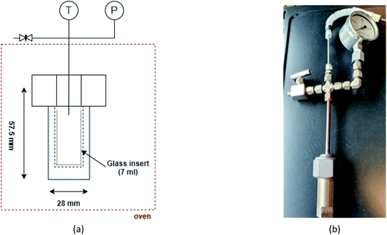Fig. 1 (a) A schematic diagram and (b) the experimental setup of the reactor tube.

Tests were designed such that (i) all reactor parts were weighed empty including the glass insert before the start of each experiment. (ii) The wet biomass was first mixed to be in the form of a homogenized slurry and then loaded onto the glass insert (with approximately 4.5 g of wet biomass). (iii) Post the assembly of the reactor, it was weighed and transferred for high-pressure operation. (iv) The reactor was flushed three times with nitrogen and was pressurized with nitrogen to 50 bar so as to perform a 15 min leak test. (v) Having carried out a successful leak test, the pressure was released to just above the atmospheric pressure, and the entire reactor assembly was finally weighed again. (vi) The reactor was then placed in a pre-heated oven at 530–600 °C and the pressure and temperature values were recorded at an interval of 1 min. (vii) After 45 min of operation, the reactor assembly was removed from the oven and cooled down to room temperature using an air fan. (viii) Having cooled the reactor, it was weighed again, and the produced gases were collected using a 50 mL syringe equipped with a stopcock valve to measure the volume of gaseous products. (ix) The gas filled syringe was weighed and the gas was then transferred to a gas chromatograph (HP 5890 series II dual column) for further analysis. The gas chromatograph employed was equipped with one Varian Capillary Column CP-PoraBond Q (L = 50 m, ID = 0.53 mm, 10 μm) and one Agilent Technologies HP-Molesieve (L = 30 m, ID = 0.53 mm, 50 μm) column wherein helium was used as the carrier gas.

Analyses were carried out for three different biomass wastes, i.e. cattle manure, fruit/vegetable waste, and cheese whey, in order to measure the influence of composition and different process parameters on the SCW gasification conversion. The proximate, ultimate, and major element analyses of the biomass wastes are presented in Table 3.

Table 3 Proximate, ultimate and major element analyses of the biomass wastes

Parameters	Cattle manure	Fruit & vegetable waste	Cheese whey
Proximate analysis
Moisture [% w/w as received (a.r.)]	82.9	89.0	97.0
Volatiles [% w/w dry basis (d.b.)]	66.0	72.4	62.1
Fixed carbon [% w/w d.b.]	15.3	20.4	19.0
Ash [% w/w d.b.]	18.7	7.2	18.9
Ultimate analysis
C [% w/w d.b.]	43.5	46.3	38.9
H [% w/w d.b.]	5.3	5.6	5.2
N tot/NH4^+ [mg L^−1]	3320/2.9	628/1.1	131/0.4
TOC [g L^−1]	8.9	27.9	16.8
COD [g L^−1]	27.7	91.1	45.7
HHV/LHV [MJ kg^−1 (d.b.)]	19.2/18.1	19.8/18.6	15.6/14.5
Major element analysis (mg kg ^−1 of biomass) (a.r.)
K	3191.0	1863.0	1417.0
Ca	3202.0	317.0	995.0
P	891.0	192.0	586.0
Mg	1604.0	152.0	130.0
Fe	289.0	—	—
S	420.0	94.8	51.4
Na	548.0	32.2	420.0
Sr	—	5.4	—
Zn	—	2.4	3.7
B	—	4.3	1.9
Al	81.7	—	0.7
Si	80.6	—	—

---

Advanced thermal equilibrium modeling

Despite the complexity of the thermochemistry of biomass conversion in supercritical water, modeling is always an important tool for a better understanding of such a complex system. Three thermodynamic modeling approaches have been pursued to assess the SCWG optimization: (i) GTE which simply uses the Gibbs free energy minimization technique and (ii) the constrained thermodynamic equilibrium model which is founded on GTE along with additional constraints and (iii) the thermal-quasi equilibrium model which is based on the concept of approach temperature. Simulations for each of the three different biomass wastes have been considered for 100 kg waste as the input with temperature and pressure ranging from 100–700 °C and 230–260 bar, respectively.

Background of the thermodynamic equilibrium modelling calculations

A closed system is said to be in its thermodynamic equilibrium when the total Gibbs free energy of the defined system is minimum with respect to all possible changes at constant pressure and temperature. Theoretically, the equilibrium state of a closed system is defined in eqn (1).

(dG^t)_P,T = 0 (1)

where (dG^t) refers to the change in the Gibbs free energy of the closed system with respect to time at constant pressure P and temperature T. Furthermore, the total Gibbs free energy of the system, which has to be minimized, can be computed using eqn (2).where G is the total Gibbs free energy of the system to be minimized, ø is the phase index, N^ø is the total molar amount of a phase and G_m^ø is the total mole-based Gibbs free energy of a phase. Therefore, the total Gibbs free energy for a typical multiphase system can be enumerated using eqn (3).where ig, pcp, and s refer to the ideal gas, pure condensed phase, and solution phase. n_i, p_i, x_i, γ_i and g⁰_i refer to the number of moles, partial pressure, mole fraction, activity coefficient, and standard molar Gibbs free energy for the i^th compound. G, R and T are the total Gibbs free energy of the system, universal gas constant, and temperature, respectively.

GTE model using FactSage™ software

In this work, we employed FactSage™ software to assess the gasification behavior for the different biomass case studies. FactSage™ is a thermochemical equilibrium software package consisting of different calculation modules and databases. The ‘equilib’ tool uses Gibbs free energy minimization for computing multicomponent equilibria, multiphase conditions with a large possible range of natural constraints. The Gibbs free energy minimization is based on the ChemApp algorithm.³⁷ The Gibbs free energy of the system, which is minimized for a combination of composition, temperature, and pressure, is expressed using eqn (3).

Calculations are separately performed for two distinct regions: (i) the subcritical region with temperatures ranging from 100–375 °C and (ii) the supercritical region with temperatures ranging from 400–700 °C. The two regions are devised based on the fact that for a selected reactor pressure of 240 bar, the pseudo-critical point of water is expected to lie in the 385–390 °C range.³⁴ The pseudo-critical point refers to the temperature where the phase transition of water is completed and the isobaric heat capacity is at its maximum.³⁸ Under subcritical reaction conditions, three different modules, FactPS, FTsalt, and FThelg, have been employed for the selection of compounds and solutions. For the supercritical region, three modules are selected, namely FactPS, FTsalt, and FToxid. FactPS provides inclusive databases for over 500 compounds. Data for the gaseous phase will generally be found in FactPS. The FTsalt module consists of data for pure salts and salt solutions, and under this module, the adopted databases are FTsalt-CSOB, FTsalt-SALTF, FTsalt-ALKN, FTsalt-ALOH, FTsalt-SCSO and FTsalt-SSUL. The FThelg module comprises infinite dilution properties of aqueous solute species based on the Helgeson equation of state which is considered for handling highly non-ideal fluid systems.³⁴ Coupled with the FThelg module, the FTHelg_AQDD database is considered. The FToxid module consists of data from all pure oxides and oxide solutions (both liquid and solid) and the databases considered are FToxid-SlagD, FToxid-C3Pa, and FToxid-C3Pr.

The GTE model is founded on Gibbs free energy minimization to predict the system behavior. The model assumes that reactions have reached chemical equilibrium, which is supposedly far from the case with a real reactor. A real gasification system deviates from its ideal system as the GTE model either over- or underestimates the gas yields due chiefly to kinetics limitations.^35,39,40 Kinetics limitations can deviate the real system from its ideal state because of different reaction rates and limited participation of carbon in the reactions. Keck and Gillespie ⁴¹ employed a similar method called rate-controlled constrained-equilibrium. The basis of the model was to combine Gibbs free energy minimization with the reaction rates of slow reactions, imposing extra constraints in the minimization routine to account for the limiting role of kinetics equations. Similarly, Koukkari et al.^42–45 applied the constrained equilibrium modelling method to improve the cross-links between reaction kinetics and thermodynamic equilibrium in a multicomponent reaction system. The authors showed that imposing constraint can lower the observed over-prediction of carbon conversion, thus alleviating serious disagreements with compositions. For such reasons, a GTE model needs to be modified by imposing constraints to potentially predict the local equilibrium state with more satisfactory precision. The advanced modeling techniques adopted for this study include constrained thermodynamic equilibrium and thermal-quasi equilibrium models and are discussed in the following sections.

Constrained thermodynamic equilibrium model

The constrained thermodynamic equilibrium method is an adaptation of the Gibbs free energy minimization by superimposing new constraints to the already existing natural constraints such as charge conservation and mole balances for the elements, and non-negativity of all the species amounts. In general, the new additional constraints can be devised and implemented in different fashions such as carbon and hydrogen gasification efficiencies, dissolved carbon conversion, and selected constant species yield values based on direct experimental measurements and multi-faceted mechanistic models. Additional constraints considered for the modeling part are discussed below.

(i) CGE – this gives an appropriate indication of how far the system from its global equilibrium is. Due to kinetics limitations, the effective carbon content participating in the reaction is less than that actually present in the biomass feed. CGE can be defined as the ratio of total number of moles of carbon in the product, e.g. CO₂, CH₄, CO, C_xH_y, to the total number of carbon moles in the biomass feedstock. Eqn (4) shows how the CGE, as an equal constraint, is superimposed to the model.

where g refers to the gas phase. n_feed refers to the total number of moles in the feed. a and m_i refer to the number of carbon atoms per molecule of the i^th species and moles of the i^th species including CO₂, CH₄, CO, and C_xH_y.

(ii) Experimental yield limits on specific compounds – due to kinetics limitations, some reactions are possibly slower than others and are termed here rate-limiting reactions. Due to different reaction rates, the formation of products is over- or underestimated. Conceptually, for the case of SCWG, formation of CH₄ is favored at lower temperatures, whilst H₂ is a favorable product at a higher temperature. This can be taken into account by considering a fixed yield of that specific compound in the model. A fixed value of the compound can be computed by conducting simple laboratory-scale experiments. Eqn (5) shows how this constraint is introduced into the model.

n_i = A (5)

where n_i and A are the number of moles of the i^th compound and the fixed experimental value of the same compound.

An advanced version of the constrained equilibrium model which uses the Gibbs free minimization technique has been developed by Yakaboylu et al.³⁵ The authors developed a MATLAB code including different sets of constraints which applies the fmincon routine to solve the optimization problem. The code uses Gibbs free energy minimization equations for gases, aqueous species, and solids phase species wherein the effects of different sets of additional constraints were considered.

Thermal-quasi equilibrium model

The basic philosophy behind the thermal-quasi equilibrium model is the estimation of CGE by representing kinetics limitations through the concept of “approach temperature” to improve the accuracy of the GTE model. Other than carbon, there is no methodical way to cater for the incomplete conversion of elements. Therefore, when using a thermal-quasi equilibrium model, complete conversion of all the elements is inevitably assumed. The concept behind approach temperature is to counterbalance the carbon conversion obtained from experimental data by considering a temperature difference between the temperature in the SCW gasifier (real reactor conditions) and a hypothetical temperature corresponding to the same gas composition from the GTE model. This difference between the two temperatures is here termed approach temperature. In fact, the concept of thermal quasi-equilibrium modelling is developed such that the deviation of the ideal GTE approach from more realistic kinetics-based methods is bridged by introducing an approach temperature, which is computed by comparing experimental results with GTE predictions, and it indicates the temperature difference between the GTE set-up and the experimental conditions, such that a similar composition for the produced gases is found. This delta T can be considered as a representative for the conceptual resistances/limitations assigned to mass, heat and momentum transport processes and thus reactions.

Gumz⁴⁶ investigated a similar approach for fluidized bed and downdraft gasifiers. In this study, the author found that the average bed temperatures could be potentially considered as the process temperatures for fluidized beds while the exit temperature at the throat of a downdraft gasifier could be a good estimate for the process temperature. Li et al.⁴⁷ investigated coal gasification and found that the carbon conversion obtained experimentally at 1020–1150 K was similar to the equilibrium predictions at 800–900 K.

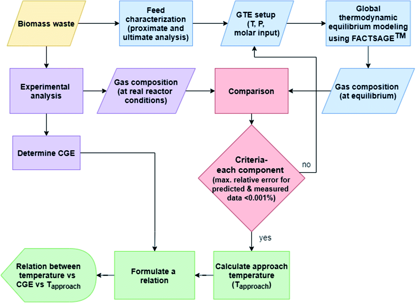
Fig. 2 elucidates the conceptual flowchart for the thermal-quasi equilibrium model used in this study. As shown in Fig. 2, biomass waste follows two different processing streams. The first processing stream includes lab-scale experiments to compute real product compositions while the second one is directed to biomass analysis, i.e. proximate and ultimate analyses. The results from these analyses are further processed, where molar quantities of the elements are fed into the GTE model using FACTSAGE™ software. The experimental results are then compared to the model predictions for each and every individual component whilst a maximum relative error of 0.001% is targeted to compute the approach temperature in a trial and error procedure. Finally, a relation is derived between actual temperature (in the reactor tube), approach temperature, and the CGE calculated based on experimental results. Using the resulted correlation, the gas product composition can be reliably predicted from one more simulation run with FACTSAGE™, although experimental analysis for determining CGE is a pre-requisite.

Fig. 2 Flowchart depicting the working principle for the thermal-quasi equilibrium model.

Results and discussion

Validation

This section aims to assess the validity of different modeling approaches by comparing the simulation results to those of experiments. To this end, validation of the models is investigated for all three feedstock cases under ‘as received’ conditions for a specific SCW gasifier temperature and pressure. It is worth mentioning that due to the purging of nitrogen and use of different amounts of feedstocks in the tests, the pressure levels varied from 230 to 260 bar, but it is known that pressure does not have a considerable effect on SCWG.³⁰Fig. 3–5 illustrate the comparative results for manure, fruit/vegetable waste, and cheese whey, respectively, where the gas yield for the main gaseous products is benchmarked against test results. Overall, the bar plots show a reasonable agreement between the test results and GTE model predictions based on FactSage™ simulations.

Fig. 3 Comparison between experimental results and FactSage™ (non-constrained) predictions for manure with a concentration of 17 wt% at 552 °C and 260 bar.

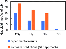Fig. 4 Comparison between experimental results and FactSage™ (non-constrained) predictions for fruit/vegetable waste with a concentration of 11 wt% at 560 °C and 240 bar.

Fig. 5 Comparison between experimental results and FactSage™ (non-constrained) predictions for cheese whey with a concentration of 3 wt% at 539 °C and 235 bar.

The observed deviation of the predicted gas yield from experimental data can be explained by the fact that GTE predicts gas compositions at the global minima of the Gibbs free energy, whilst in a real reactor environment local equilibrium does not occur. We therefore expect that the results of thermal equilibrium modeling can be improved by imposing additional constraints to account for the role of CGE, which is covered in the next section.

Gas behavior

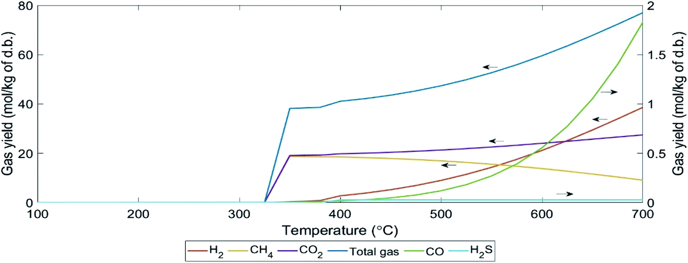
GTE approach. Simulations for the different biomass (manure, fruit/vegetable waste, sewage, and cheese whey) were conducted using FACTSAGE™ at a pressure of 240 bar and a temperature range of 100–700 °C and the results are illustrated in Fig. 6–8. The product gas is mainly composed of CO₂, CO, H₂, CH₄, and H₂S, whereas other species such as N₂, NH₃ (not shown in the figures) are also produced in small quantities. Overall, the results show that the total gas yield significantly increases above 300 °C, which is ascribed to the drastic decrease of solid carbon in this range of temperature. Similar behavior is reported by other research groups.^{21,26,34,35,40} Furthermore, several research groups, e.g. Guo et al.,²⁴ Peomdej et al.,⁴⁸ and Nanda et al.,²⁶ have reported that the density of water decreases above its critical point, resulting in the disruption of ionic product formation. In fact, the decreased formation of ionic products enhances free radical mechanisms, and thus leads to a higher yield of gases.

Fig. 6 Behavior of different gases released during the SCWG of manure with a concentration of 17 wt% at 240 bar and in the temperature range of 100–700 °C. The results are based on GTE conditions using FACTSAGE™ simulations.

Fig. 7 Behavior of different gases released during the SCWG of fruit/vegetable waste with a concentration of 11 wt% at 240 bar and in the temperature range of 100–700 °C. The results are based on GTE conditions using FACTSAGE™ simulations.

Fig. 8 Behavior of different gases released during the SCWG of cheese whey with a concentration of 3 wt% at 240 bar and in the temperature range of 100–700 °C. The results are based on GTE conditions using FACTSAGE™ simulations.

Methane gas yields for all three types of biomasses demonstrate a decline at temperatures higher than 400 °C, whilst those of CO and H₂ reveal an increasing trend. This can be explained by the backward methanation reaction which consumes methane and water to form hydrogen and carbon monoxide (see eqn (6)). High hydrogen yields are justified as the water gas shift reaction (see eqn (7)) is enhanced at higher temperatures and also the possible hydrogen formation routes increase due to the thermal decomposition of intermediates, as suggested by Acelas et al.⁴⁹ The increase in carbon dioxide yields at higher temperatures is attributed to the enhanced forward water gas shift reaction in the higher temperature range (eqn (7)). The overall trend and behavior of the main gaseous products for all three biomasses show a good agreement with literature findings reported by Acelas et al.,⁴⁹ Guo et al.,²⁴ Cao et al.,⁵⁰ and Yakaboylu et al.³⁴

CO + 3H₂ ↔ CH₄ + H₂O (6)

CO + H₂O ↔ CO₂ + H₂ (7)

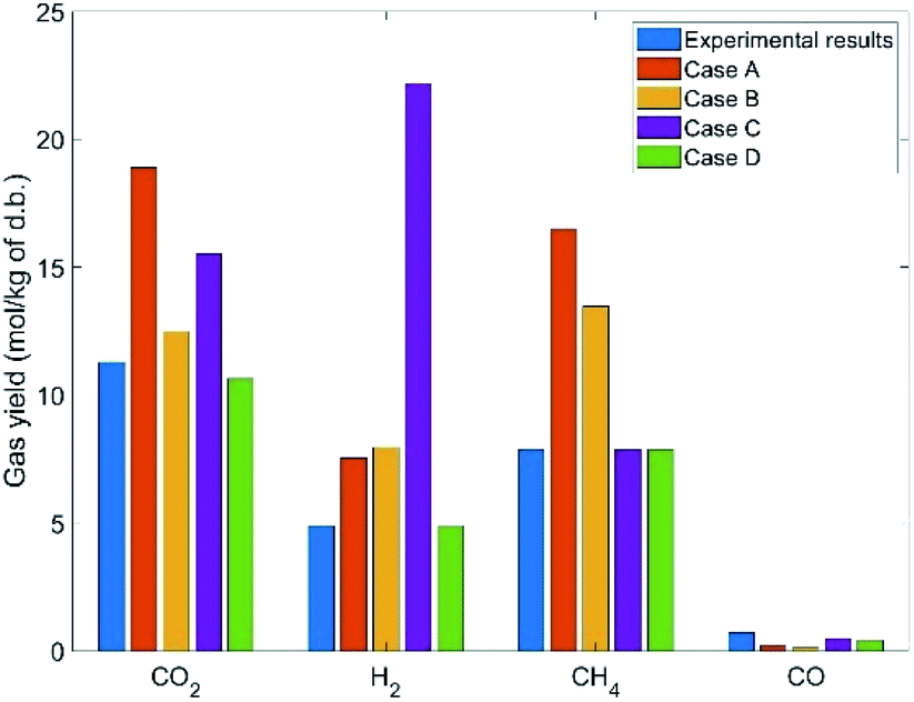
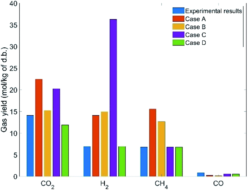
Constrained thermodynamic equilibrium approach. Fig. 9–11 show the comparison of the results for the main gaseous product behavior predicted by constrained and unconstrained (FactSage™ Simulations) models and the experimental data for all the biomass. The comparison analysis for each biomass type was conducted at specific temperature and pressure, and additional results for other ranges of temperature and pressure are provided in ESI A1† for the sake of brevity. Our analyses include different case studies for each biomass type wherein Case A involves no additional constraints and gas compositions are based on the GTE approach, Case B applies CGE as the only additional constraint, Case C uses CGE along with a specific amount of CH₄ obtained from experiments as additional constraints and Case D uses CGE together with specific amounts of CH₄ and H₂, obtained from experiments, as additional constraints. It is worth noting that CGE values are determined using experimental data. The overall view of the data used for the constraint equilibrium model is presented in Table 4.

Fig. 9 Comparisons between different modeling approaches and experimental values for manure at 552 °C and 260 bar with a feed concentration of 17 wt%. Case A includes only GTE values, Case B includes CGE as a constraint, Case C includes CGE + a constant amount of CH₄ as constraints, Case D includes CGE + a constant amount of CH₄ and H₂ as constraints.

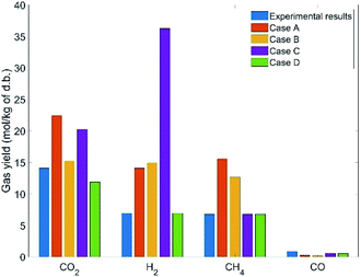Fig. 10 Comparisons between different modeling approaches and experimental values for fruit/vegetable waste at 560 °C and 240 bar with a feed concentration of 11 wt%. Case A includes only GTE values, Case B includes CGE as a constraint, Case C includes CGE + a constant amount of CH₄ as constraints, Case D includes CGE + a constant amount of CH₄ and H₂ as constraints.

Fig. 11 Comparisons between different modeling approaches and experimental values for cheese whey at 539 °C and 235 bar with a feed concentration of 3 wt%. Case A includes only GTE values, Case B includes CGE as a constraint, Case C includes CGE + a constant amount of CH₄ as constraints, Case D includes CGE + a constant amount of CH₄ and H₂ as constraints.

Table 4 Additional constraint values used for modeling

Biomass feed	Experimental conditions (T (°C)/P (bar))	CGE (%)	CH4 amount (mol kgbiomass^−1 on d.b.)	H2 amount (mol kgbiomass^−1 on d.b.)
Manure	552/260	86.0	6.4	10.9
Fruit/vegetable waste	560/240	83.3	8.1	8.3
Cheese whey	539/235	83.9	9.1	9.2

---

As evident in Fig. 9–11, the GTE approach (Case A) does not show the expected satisfactory agreement with the experimental gas compositions for all the biomass feed campaigns. It can also be observed that the expected improvement in the accuracy of predictions for Cases B and C is not satisfactory. However, the predictive results from Case D reveal very good agreement with the experimental values. In fact, results of Case D substantiate that superimposing CGE and experimental values of CH₄ and H₂ into the model results in an accurate prediction of the product gas (see Table 5). Similar findings have been reported by Yakaboylu et al.³⁵ Deviations of the predictive results for different constraint cases from experimental values are reported in Table 5. These results demonstrate that the accuracy of predictions improved significantly in Case D compared with Cases A, B, and C.

Table 5 Deviations based on the product gas concentrations for the three biomass wastes in all four different cases

Deviations from experimental results (%)
Product gas	Case A	Case B	Case C	Case D
Manure
CO2	52.0	32.3	53.1	19.9
H2	36.5	42.1	224.9	0.0
CH4	48.4	32.5	0.0	0.0
CO	−70.0	−73.8	−28.8	−23.8
Fruit/vegetable waste
CO2	55.0	23.1	53.9	0.3
H2	111.5	97.1	333.6	0.0
CH4	82.7	65.0	0.0	0.0
CO	−69.0	−70.3	−17.2	−6.9
Cheese whey
CO2	126.0	103.9	64.3	29.2
H2	336.6	325.3	133.6	0.0
CH4	−27.8	−48.7	0.0	0.0
CO	−75.6	−79.5	−91.0	−23.1

---

Thermal-quasi equilibrium approach. To understand the concept of “approach temperature”, experimental gas compositions along with CGE are further processed and analyzed. First, the results from experimental gas compositions and calculated CGE shown in Fig. 12 are fitted to a temperature-dependent function using simple curve fitting techniques. For the analysis, four experimental data sets for fruit/vegetable waste are considered. Based on the nature of the data, exponential and logarithmic curve fitting functions have been utilized leading to an R-squared (R²) value of at least 0.75. The CGE and gas composition results, illustrated in Fig. 12, show a very good agreement with the experimental data of Nanda et al.^16,26 where the authors gasified fruit/vegetable waste and fructose as model compounds representing fruit/vegetable waste under critical conditions. They also reported that CGE increases with an increase in temperature, expectedly.

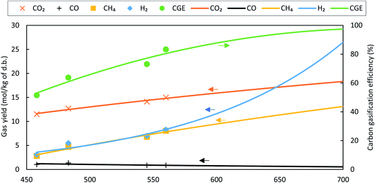Fig. 12 CGE and measured gas composition as a function of reactor temperature for fruit/vegetable waste at 240 bar with a feed concentration of 11 wt%. The experimental data for CO₂, CO, CH₄, H₂ and CGE are also represented. The gas yields and CGE plots are based on a curve fit.

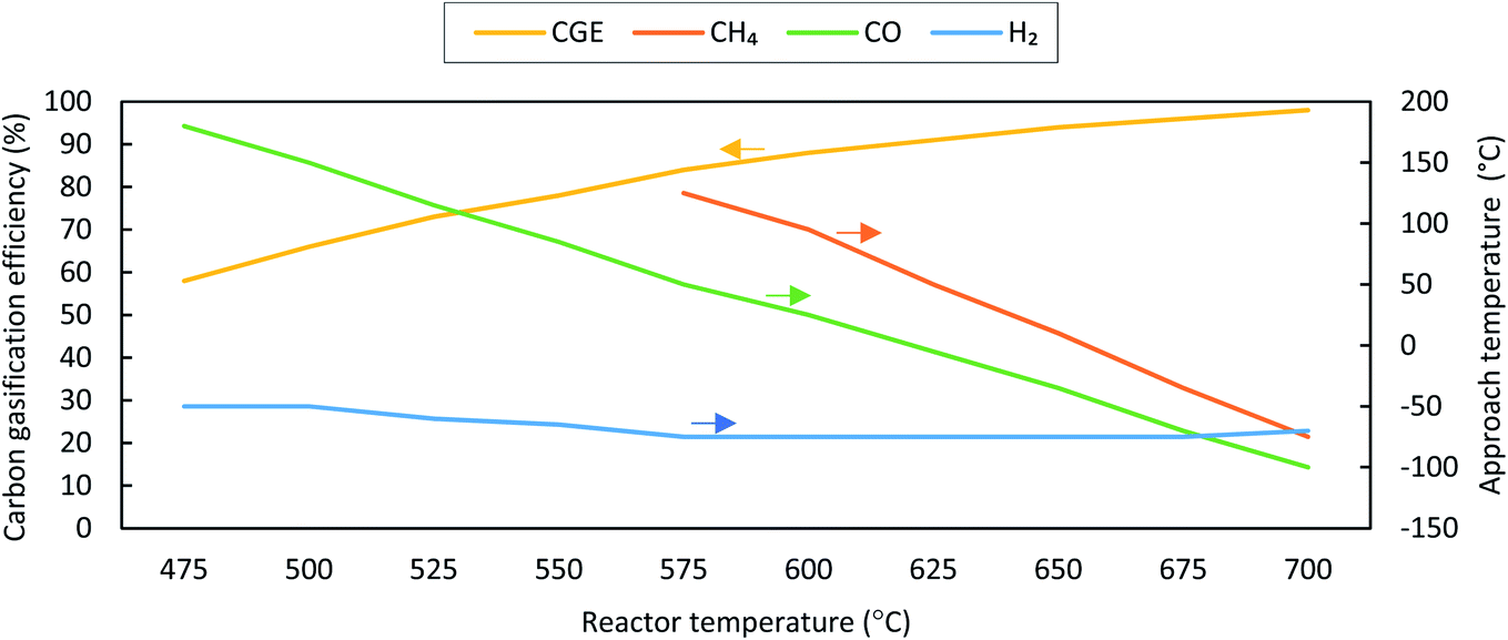
While comparing the composition results, gas compositions obtained from experiments are found to be comparable with GTE compositions predicted by FACTSAGE™ simulations with a temperature deviation of up to +180 °C and −100 °C. This temperature deviation is called “approach temperature”. Taking the particular case of SCWG of fruit/vegetable waste for computing the approach temperature, it is observed that the H₂ composition (mol kg⁻¹, d.b.) computed using the GTE model (based on FACTSAGE™ simulation) at 525 °C is similar to the experimental H₂ composition (mol kg⁻¹, d.b.) at 600 °C and thus the approach temperature is −75 °C. This is also indicated in Fig. 13. Based on this comparative analysis, a relation among the CGE, approach temperature, and reactor temperature has been derived, and is shown in Fig. 13. The figure illustrates the absolute approach temperature values for CH₄, CO, and H₂ along with CGE as a function of reactor temperature. One can use the relation shown in Fig. 13 to realize a few of the most important parameters, such as CGE and product gas compositions in a real reactor. For example, if the estimation of the real reactor conditions and product gas behaviour at 600 °C are questioned, then one can use the relation to find the CGE value which comes around 90%. Moreover, one can estimate the concentration of product gases (e.g., like for the case of CH₄) where the approach temperature is approximately 95 °C. Therefore, the composition (mol kg⁻¹, d.b.) of CH₄ will be equal to the GTE predicted composition (mol kg⁻¹, d.b.) at 695 °C (calculated using reactor temperature + approach temperature), which can be obtained from FACTSAGE™ results. A similar method can be employed to estimate the composition of other gases for the real reactor conditions.

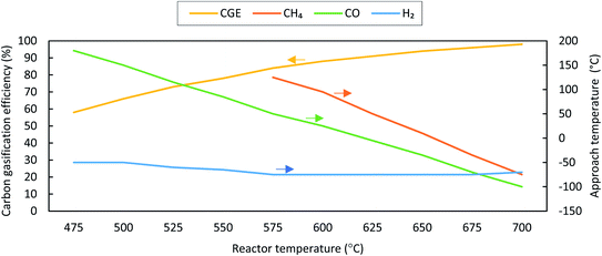Fig. 13 Absolute values of approach temperatures and CGE as a function of reactor temperature for fruit/vegetable waste at 24 MPa with a feed concentration of 11 wt%.

In general, the thermal-quasi equilibrium approach provides some advantages over the constrained thermodynamic model. In terms of accuracy, the thermal quasi-equilibrium model gives the exact experimental data point as the approach temperature is calculated based on the basis of similar data (see Fig. 12); however, the use of even three additional constraints in the constraint equilibrium model results in deviation for the predicted CO and CO₂ compositions (see Table 5, e.g., deviation in the CO₂ composition of cheese whey). However, the main advantage of the thermal-quasi equilibrium model is its credibility for scale-up calculation, where the approach temperature can guarantee the reproducibility of the results of pilot or lab-scale experiments for industrial-scale SCW gasifiers. Furthermore, the accuracy of the constrained thermal equilibrium model is highly dependent on the number of constraints imposed into the model. The other advantage of the thermal-quasi equilibrium approach is the ease of implementation. In fact, the model offers an effective approach temperature to lump all the constraints used in the constrained equilibrium model.

Element behavior

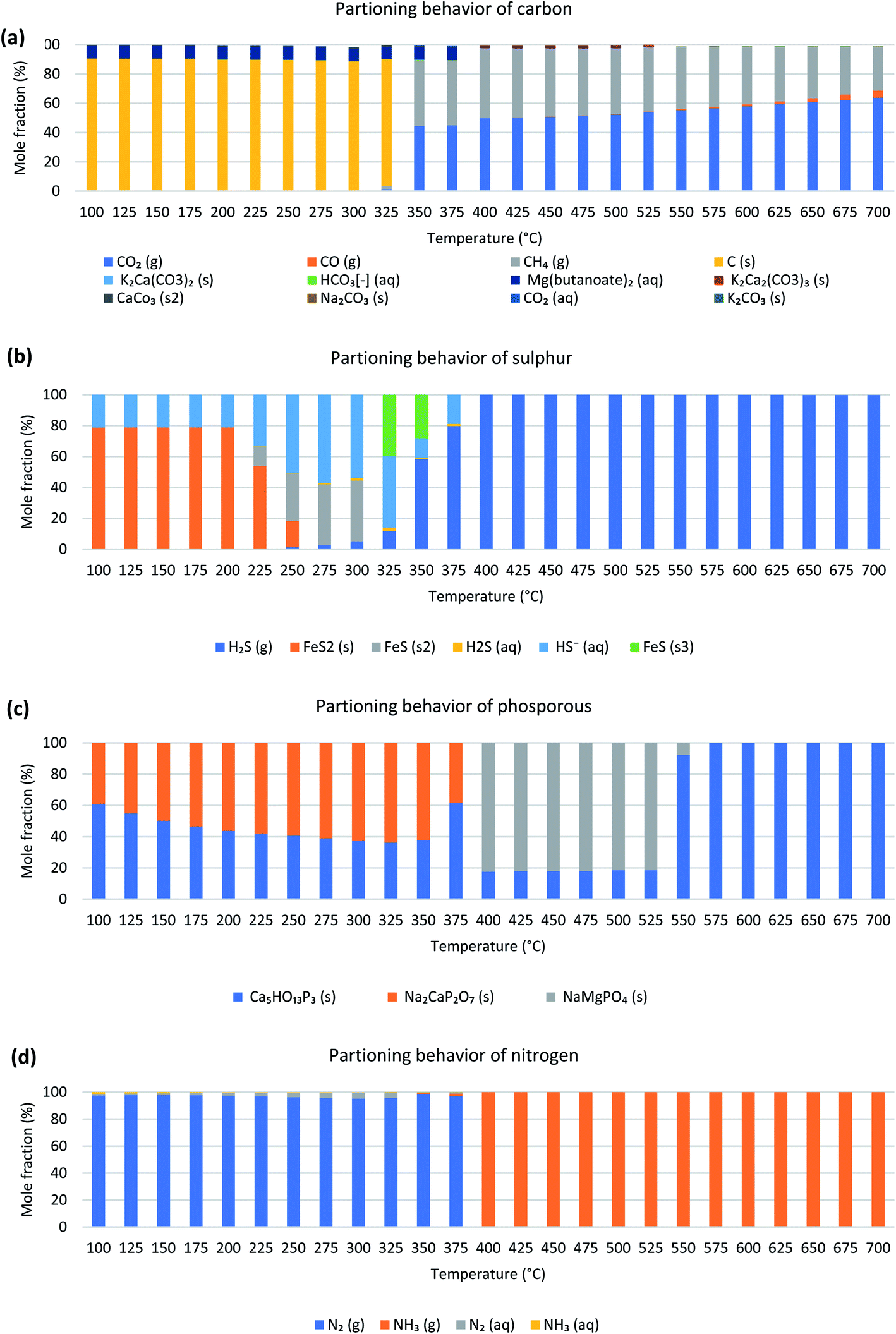
GTE approach. The distribution of elements such as carbon, sodium, magnesium, calcium, phosphorus and other inorganic elements is investigated in this section. The basis of the partitioning assessment is the GTE approach. Such information is of high interest as it assists in the evaluation of ash and slag formation and their predicted compositions. Moreover, precipitation of mineral content present in the biomass feedstock can lead to reactor plugging during operation.³⁴ Furthermore, such results can assist in a better quantification of the operating parameters for SCW reactors, and, in principle, for potential reduction of the amount of solid residues to be further processed or disposed of. More importantly, using this study on partitioning behavior, one can develop a material and substance flow analysis for systematic assessment of the stocks and flows of materials within a biorefinery unit.⁵¹Fig. 14(a–d) illustrate the elemental partitioning behavior results for manure. The partitioning behavior for manure (remaining elements), fruit/vegetable waste and cheese whey is discussed in ESI B1–B3† for the sake of brevity. These results are based on the SCWG of biomass wastes at 240 bar and in the temperature range of 100–700 °C. For this purpose, FactSage™ simulations are performed under subcritical conditions for the temperature range of 100–375 °C whilst the range of 400–700 °C is considered for supercritical conditions.

Fig. 14 Partitioning behavior of (a) carbon, (b) sulfur, (c) phosphorus, and (d) nitrogen compounds during SCWG of manure in the temperature range of 100–700 °C at 24 MPa with a concentration of 17 wt%.

As shown in Fig. 14(a), the first region which lies between 100 and 325 °C is dominated by solid carbon in the form of graphite along with small amounts of Mg(butanoate)₂ and CaCO₃. While the second region in the range of 350–700 °C shows the dominance of gas products such as CO₂, CH₄, and CO followed by the appearance of compounds such as Na₂CO₃, K₂Ca₂(CO₃)₃, K₂CO₃, and HCO₃⁻ in small quantities. At temperatures higher than 350 °C solid carbon decomposes to form CO₂ and CH₄. CH₄ further starts decomposing around 400 °C and gets converted into CO₂, CO and H₂.

Partitioning behavior of sulfur is shown in Fig. 14(b). At temperatures lower than 225 °C, mainly FeS₂ is present in the fraction along with smaller quantities of FeS (s2) and HS⁻. At temperatures higher than 225 °C, sulfur further decomposes to compounds like FeS (s3), aqueous H₂S, and HS⁻. In the supercritical region, sulfur is only present in the gaseous form of H₂S.

As shown in Fig. 14(c) phosphorus compounds are only present in solid form in the entire gasification temperature range. At temperatures lower than 375 °C, phosphorus is present only in two forms, i.e., Ca₅(OH)(PO₄)₃ and Na₂CaP₂O₇ with an average of 45% and 54%, respectively. Between 400 °C and 525 °C, the region is dominated by NaMgPO₄ along with smaller quantities of Ca₅(OH)(PO₄)₃. At temperatures exceeding 550 °C, Ca₅(OH)(PO₄)₃ is the only stable form of phosphorus.

The partitioning behavior of nitrogen is shown in Fig. 14(d). As illustrated in this figure, nitrogen in the form of N₂ gas is the most stable compound present at temperatures below 375 °C along with smaller quantities of aqueous N₂ and NH₃. At temperatures exceeding 400 °C, the only compound present is NH₃ (g). Such a finding has previously been reported by Yakaboylu et al.³⁵ and Klingler et al.⁵² Yakaboylu et al.³⁵ highlighted that nitrogen is only released in the form of NH₃ during the gasification of biomass. Klingler et al.⁵² mention that under hydrothermal conditions when amino acids react with water, NH₃ is formed. Therefore, N₂ is deselected for supercritical conditions in the FACTPS module.

Conclusion

Detailed multiphase-thermodynamic equilibrium models for SCWG of different-source biomass types including cattle manure, fruit/vegetable waste, and cheese whey have been developed to investigate the behavior of produced gas under different reactor conditions. The models are founded on Gibbs free energy minimization and further improved to account for CGE, resulting in constrained and thermal-quasi equilibrium models. The conceptual models were then validated and improved based on a supplementary experimental study. Overall, both theoretical and experimental analyses substantiate the important role of temperature in the final yield of the products and CGE. Furthermore, comparison between analytical and experimental results demonstrated a discernible improvement in the prediction of the GTE model by imposing additional constraints to the model and by using the concept of approach temperature to the model. For the constrained equilibrium model, the results show that by increasing the number of constraints, the predictability of the model tremendously improves, although at the expense of reliance on more experimental data points. For example, the deviation of CO₂ yield from experimental data significantly improved from 55% to 0.3% for fruit/vegetable residue gasification by imposing all three constraints to the GTE model. The concept of the thermal-quasi equilibrium model was also elaborated, offering the lumping of all additional constraints used in the constrained equilibrium model into approach temperature. Overall, the comparison results also demonstrated a better prediction of the thermal quasi-equilibrium model than that of constrained and GTE models for the gas composition of the available experimental data points. This can be explained by the fact that the constrained model only considers water–gas shift and methanation reactions which are not the only reaction pathways in the SCWG process and thereby cannot thoroughly compensate the limitations of mass, heat, and momentum transport and thus reactions. This was the main reason for the observed deviations of the predicted CO and CO₂ yields by the constraint equilibrium model from the experimental data. However, the mentioned limitations can be represented by the approach temperature, which assists in the reproduction of the exact experimental data points. More importantly, the advantage of the thermal-quasi equilibrium model is its credibility for scale-up calculation, where the approach temperature can guarantee the reproducibility of the results of pilot or lab-scale experiments for industrial-scale SCW gasifiers while GTE and constrained models can hardly assist in scale-up calculations.

Conflicts of interest

There are no conflicts to declare.

Nomenclature

Abbreviations

a.r.	As received
BOD	Biochemical oxygen demand
CGE	Carbon gasification efficiency
COD	Chemical oxygen demand
d.b.	Dry basis
EOS	Equation of state
GTE	Global thermodynamic equilibrium
HHV	Higher heating value
LHV	Lower heating value
SCW	Supercritical water
SCWG	Supercritical water gasification
TOC	Total organic carbon

Symbols

ig	Ideal gas
pcp	Pure condensed phase
s	Solution phase
n	Moles
p	Partial pressure
x	Mole fraction
g	Gas phase
a	Carbon atoms per molecule
m	Number of carbon atoms
g ^0	Standard molar Gibbs free energy
A	Fixed experimental value of the compound
G	Total Gibbs free energy
N	Total molar amount of a phase
P	Pressure
R	Universal gas constant
T	Temperature
γ	Activity coefficient
ø	Phase

Subscripts

i	Compound i
feed	Biomass feed

Acknowledgements

The authors acknowledge NOW-ENW for the provision of financial support during the course of this project. The research is co-funded within the framework of the EU FACCE-SURPLUS Super value project (contract number ALW.FACCE.15).

Notes and references

1. International Energy Agency, World Energy Outlook, 2019, [cited 2020 May 10], available from: https://webstore.iea.org/world-energy-outlook-2019.
2. Global Bioenergy Statistics, WBA Global Bioenergy Statistics 2018, World Bioenergy Assoc, 2018, p. 43, available from: https://worldbioenergy.org/uploads/181017%20WBA%20GBS%202018_Summary_hq.pdf.
3. M. Blakeney, Food loss and food waste: Causes and solutions, 2019, pp. 1–204,  DOI:10.1111/deve.12212.
4. R. Chainey, in Which countries waste the most food, World Economic Forum, 2015, pp. 1–3.
5. FAO, Food wastage footprint & Climate Change, 2011, vol. 1, pp. 1–4, available from: http://www.fao.org/3/a-bb144e.pdf.
6. D. M. Berendes, P. J. Yang, A. Lai, D. Hu and J. Brown, Estimation of global recoverable human and animal faecal biomass, Nat. Sustainability, 2018, 1(11), 679–685,  DOI:10.1038/s41893-018-0167-0.
7. I. Lappa, A. Papadaki, V. Kachrimanidou, A. Terpou, D. Koulougliotis and E. Eriotou, et al., Cheese Whey Processing: Integrated Biorefinery Concepts and Emerging Food Applications, Foods, 2019, 8(8), 347 , available from: https://www.mdpi.com/2304-8158/8/8/347.
8. G. Lopez, M. Artetxe, M. Amutio, J. Alvarez, J. Bilbao and M. Olazar, Recent advances in the gasification of waste plastics. A critical overview, Renewable Sustainable Energy Rev., 2018, 82, 576–596 , available from: https://linkinghub.elsevier.com/retrieve/pii/S1364032117312832.
9. O. Yakaboylu, J. Harinck, K. Smit and W. de Jong, Supercritical Water Gasification of Biomass: A Literature and Technology Overview, Energies, 2015, 8(2), 859–894 , available from: http://www.mdpi.com/1996-1073/8/2/859.
10. Y. Matsumura, Hydrothermal Gasification of Biomass, Recent Advances in Thermochemical Conversion of Biomass, Elsevier Inc., 2015, pp. 251–267,  DOI:10.1016/B978-0-12-396488-5.00009-5.
11. Y. Yoshida, K. Dowaki, Y. Matsumura, R. Matsuhashi, D. Li and H. Ishitani, et al., Comprehensive comparison of efficiency and CO2 emissions between biomass energy conversion technologies—position of supercritical water gasification in biomass technologies, Biomass Bioenergy, 2003, 25(3), 257–272 , available from: https://linkinghub.elsevier.com/retrieve/pii/S0961953403000163.
12. Y. Matsumura, Fundamental design of a continuous biomass gasification process using a supercritical water fluidized bed, Int. J. Hydrogen Energy, 2004, 29(7), 701–707 , available from: https://linkinghub.elsevier.com/retrieve/pii/S0360319903002416.
13. M. Magdeldin, T. Kohl, C. De Blasio, M. Järvinen, S. W. Park and R. Giudici, The BioSCWG project: understanding the trade-offs in the process and thermal design of hydrogen and synthetic natural gas production, Energies, 2016, 9(10), 1–27,  DOI:10.3390/en9100838.
14. Y. Lu, L. Guo, X. Zhang and Q. Yan, Thermodynamic modeling and analysis of biomass gasification for hydrogen production in supercritical water, Chem. Eng. J., 2007, 131(1–3), 233–244 , available from: https://linkinghub.elsevier.com/retrieve/pii/S1385894706005079.
15. A. Kruse, Supercritical water gasification, Biofuels, Bioprod. Biorefin., 2008, 2(5), 415–437,  DOI:10.1002/bbb.93.
16. S. Nanda, S. N. Reddy, H. N. Hunter, A. K. Dalai and J. A. Kozinski, Supercritical water gasification of fructose as a model compound for waste fruits and vegetables, J. Supercrit. Fluids, 2015, 104, 112–121,  DOI:10.1016/j.supflu.2015.05.009.
17. M. Modell, Processing methods for the oxidation of organics in supercritical water, US Pat., US4543190A, 1982, available from: https://patents.google.com/patent/US4543190A/en.
18. M. Modell, R. C. Reid and S. I. Amin, Gasification process, US Pat., 4113446, USA, 1978, available from: https://patents.google.com/patent/US4113446A/en.
19. T. B. Thomason and M. Modell, Supercritical Water Destruction of Aqueous Wastes, Hazard. Waste, 1984, 1(4), 453–467,  DOI:10.1089/hzw.1984.1.453.
20. Y. Matsumura, T. Minowa, X. Xu, F. W. Nuessle, T. Adschiri and M. J. Antal, High-pressure carbon dioxide removal in supercritical water gasification of biomass, in Developments in thermochemical biomass conversion, Springer, 1997, pp. 864–877, available from: https://link.springer.com/chapter/10.1007/978-94-009-1559-6_69.
21. B. M. Kabyemela, T. Adschiri, R. M. Malaluan and K. Arai, Glucose and fructose decomposition in subcritical and supercritical water: detailed reaction pathway, mechanisms, and kinetics, Ind. Eng. Chem. Res., 1999, 38(8), 2888–2895,  DOI:10.1021/ie9806390.
22. M. J. Antal Jr, S. G. Allen, D. Schulman, X. Xu and R. J. Divilio, Biomass gasification in supercritical water, Ind. Eng. Chem. Res., 2000, 39(11), 4040–4053 , available from: http://www.adktroutguide.com/files/2000_Biomass_Gasification_in_Supercritical_Water.pdf.
23. T. Mizuno, M. Goto, A. Kodama and T. Hirose, Supercritical Water Oxidation of a Model Municipal Solid Waste, Ind. Eng. Chem. Res., 2000, 39(8), 2807–2810,  DOI:10.1021/ie0001117.
24. Y. Guo, S. Z. Wang, D. H. Xu, Y. M. Gong, H. H. Ma and X. Y. Tang, Review of catalytic supercritical water gasification for hydrogen production from biomass, Renewable Sustainable Energy Rev., 2010, 14(1), 334–343 , available from: https://linkinghub.elsevier.com/retrieve/pii/S1364032109002123.
25. O. Yakaboylu, I. Albrecht, J. Harinck, K. G. Smit, G.-A. Tsalidis and M. Di Marcello, et al., Supercritical water gasification of biomass in fluidized bed: first results and experiences obtained from TU Delft/Gensos semi-pilot scale setup, Biomass Bioenergy, 2018, 111, 330–342,  DOI:10.1016/j.biombioe.2016.12.007.
26. S. Nanda, J. Isen, A. K. Dalai and J. A. Kozinski, Gasification of fruit wastes and agro-food residues in supercritical water, Energy Convers. Manage., 2016, 110, 296–306,  DOI:10.1016/j.enconman.2015.11.060.
27. A. Amrullah and Y. Matsumura, Supercritical water gasification of sewage sludge in continuous reactor, Bioresour. Technol., 2018, 249, 276–283,  DOI:10.1016/j.biortech.2017.10.002.
28. A. Molino, M. Migliori, A. Blasi, M. Davoli, T. Marino and S. Chianese, et al., Municipal waste leachate conversion via catalytic supercritical water gasification process, Fuel, 2017, 206, 155–161,  DOI:10.1016/j.fuel.2017.05.091.
29. Y. Chen, L. Guo, W. Cao, H. Jin, S. Guo and X. Zhang, Hydrogen production by sewage sludge gasification in supercritical water with a fluidized bed reactor, Int. J. Hydrogen Energy, 2013, 38(29), 12991–12999,  DOI:10.1016/j.ijhydene.2013.03.165.
30. H. Tang and K. Kitagawa, Supercritical water gasification of biomass: thermodynamic analysis with direct Gibbs free energy minimization, Chem. Eng. J., 2005, 106(3), 261–267 , available from: https://linkinghub.elsevier.com/retrieve/pii/S1385894704004048.
31. T. Yanagida, T. Minowa, A. Nakamura, Y. Matsumura and Y. Noda, Behavior of Inorganic Elements in Poultry Manure during Supercritical Water Gasification, J. Jpn. Inst. Energy, 2008, 87(9), 731–736 , available from: http://joi.jlc.jst.go.jp/JST.JSTAGE/jie/87.731?from=CrossRef.
32. O. Yakaboylu, G. Yapar, M. Recalde, J. Harinck, K. G. Smit and E. Martelli, et al., Supercritical water gasification of biomass: an integrated kinetic model for the prediction of product compounds, Ind. Eng. Chem. Res., 2015, 54(33), 8100–8112.
33. O. Yakaboylu, J. Harinck, K. G. Smit and W. de Jong, Supercritical Water Gasification of Biomass: A Thermodynamic Model for the Prediction of Product Compounds at Equilibrium State, Energy Fuels, 2014, 28(4), 2506–2522,  DOI:10.1021/ef5003342.
34. O. Yakaboylu, J. Harinck, K. G. Gerton Smit and W. de Jong, Supercritical water gasification of manure: a thermodynamic equilibrium modeling approach, Biomass Bioenergy, 2013, 59, 253–263,  DOI:10.1016/j.biombioe.2013.07.011.
35. O. Yakaboylu, J. Harinck, K. G. Smit and W. De Jong, Testing the constrained equilibrium method for the modeling of supercritical water gasification of biomass, Fuel Process Technol., 2015, 138, 74–85,  DOI:10.1016/j.fuproc.2015.05.009.
36. O. Yakaboylu, J. Harinck, K. G. Smit and W. de Jong, Supercritical Water Gasification of Biomass: A Detailed Process Modeling Analysis for a Microalgae Gasification Process, Ind. Eng. Chem. Res., 2015, 54(21), 5550–5562,  DOI:10.1021/acs.iecr.5b00942.
37. G. Eriksson, K. Hack and S. Petersen, Chemapp—a programmable thermodynamic calculation interface, Werkst Woche, 1997, 96, 47–51 , available from: https://gtt-technologies.de/ca-doc/index.html.
38. M. Hodes, P. A. Marrone, G. T. Hong, K. A. Smith and J. W. Tester, Salt precipitation and scale control in supercritical water oxidation—Part A: fundamentals and research, J. Supercrit. Fluids, 2004, 29(3), 265–288 , available from: https://linkinghub.elsevier.com/retrieve/pii/S0896844603000937.
39. M. P. Arnavat, Performance modelling and validation of biomass gasifiers for trigeneration plants, 2011, available from: http://repositori.urv.cat/fourrepopublic/search/item/TDX%3A1003.
40. Q. Yan, L. Guo and Y. Lu, Thermodynamic analysis of hydrogen production from biomass gasification in supercritical water, Energy Convers. Manage., 2006, 47(11–12), 1515–1528 , available from: https://linkinghub.elsevier.com/retrieve/pii/S0196890405001950.
41. J. C. Keck and D. Gillespie, Rate-controlled partial-equilibrium method for treating reacting gas mixtures, Combust. Flame, 1971, 17(2), 237–241 , available from: https://linkinghub.elsevier.com/retrieve/pii/S0010218071801669.
42. P. Koukkari and R. Pajarre, Calculation of constrained equilibria by Gibbs energy minimization, CALPHAD: Comput. Coupling Phase Diagrams Thermochem., 2006, 30(1), 18–26.
43. P. Koukkari and R. Pajarre, Introducing mechanistic kinetics to the Lagrangian Gibbs energy calculation, Comput. Chem. Eng., 2006, 30(6–7), 1189–1196 , available from: https://linkinghub.elsevier.com/retrieve/pii/S0098135406000500.
44. P. Koukkari and R. Pajarre, A Gibbs energy minimization method for constrained and partial equilibria, Pure Appl. Chem., 2011, 83(6), 1243–1254 , available from: https://www.degruyter.com/view/journals/pac/83/6/article-p1243.xml.
45. P. Koukkari, R. Pajarre and P. Blomberg, Reaction rates as virtual constraints in Gibbs energy minimization, Pure Appl. Chem., 2011, 83(5), 1063–1074 , available from: https://www.degruyter.com/view/journals/pac/83/5/article-p1063.xml.
46. W. Gumz, Gas producers and blast furnaces: theory and methods of calculation, Wiley, 1950, available from: https://catalog.hathitrust.org/Record/001043659/Home.
47. X. Li, J. Grace, A. Watkinson, C. Lim and A. Ergüdenler, Equilibrium modeling of gasification: a free energy minimization approach and its application to a circulating fluidized bed coal gasifier, Fuel, 2001, 80(2), 195–207 , available from: https://linkinghub.elsevier.com/retrieve/pii/S0016236100000740.
48. C. Peomdej, A. Chuntanapum and Y. Matsumura, Effect of Temperature on Tarry Material Production of Glucose in Supercritical Water Gasification, J. Jpn. Inst. Energy, 2010, 89(12), 1179–1184 , available from: http://joi.jlc.jst.go.jp/JST.JSTAGE/jie/89.1179?from=CrossRef.
49. N. Y. Acelas, D. P. López, D. W. F. Brilman, S. R. A. Kersten and A. M. J. Kootstra, Supercritical water gasification of sewage sludge: Gas production and phosphorus recovery, Bioresour. Technol., 2014, 174, 167–175 , available from: https://linkinghub.elsevier.com/retrieve/pii/S096085241401414X.
50. W. Cao, C. Cao, L. Guo, H. Jin, M. Dargusch and D. Bernhardt, et al., Hydrogen production from supercritical water gasification of chicken manure, Int. J. Hydrogen Energy, 2016, 41(48), 22722–22731 , available from: https://linkinghub.elsevier.com/retrieve/pii/S0360319916327458.
51. U. Arena and F. Di Gregorio, Element partitioning in combustion- and gasification-based waste-to-energy units, Waste Manage., 2013, 33(5), 1142–1150,  DOI:10.1016/j.wasman.2013.01.035.
52. D. Klingler, J. Berg and H. Vogel, Hydrothermal reactions of alanine and glycine in sub- and supercritical water, J. Supercrit. Fluids, 2007, 43(1), 112–119 , available from: https://linkinghub.elsevier.com/retrieve/pii/S0896844607001738.

---

Footnotes

† Electronic supplementary information (ESI) available: A1 and B1, B2, and B3 provide more details about gas behavior obtained using constrained thermodynamic equilibrium modelling and element partitioning behavior, respectively. See DOI: 10.1039/d0se01635g

‡ Total efficiency is defined as the sum of the mechanical, electrical and useful thermal energy production divided by the energy produced from the input fuel.

---