 Open Access Article
Accelerated AI development for autonomous materials synthesis in flow†‡
Robert W.
Epps
 a,
Amanda A.
Volk
a,
Kristofer G.
Reyes
b and
Milad
Abolhasani
a,
Amanda A.
Volk
a,
Kristofer G.
Reyes
b and
Milad
Abolhasani
 *a
*a
aDepartment of Chemical and Biomolecular Engineering, North Carolina State University, Raleigh, North Carolina 27606, USA. E-mail: abolhasani@ncsu.edu; Web: http://www.abolhasanilab.com
bDepartment of Materials Design and Innovation, University at Buffalo, Buffalo, New York 14260, USA
First published on 9th March 2021
Abstract
Autonomous robotic experimentation strategies are rapidly rising in use because, without the need for user intervention, they can efficiently and precisely converge onto optimal intrinsic and extrinsic synthesis conditions for a wide range of emerging materials. However, as the material syntheses become more complex, the meta-decisions of artificial intelligence (AI)-guided decision-making algorithms used in autonomous platforms become more important. In this work, a surrogate model is developed using data from over 1000 in-house conducted syntheses of metal halide perovskite quantum dots in a self-driven modular microfluidic material synthesizer. The model is designed to represent the global failure rate, unfeasible regions of the synthesis space, synthesis ground truth, and sampling noise of a real robotic material synthesis system with multiple output parameters (peak emission, emission linewidth, and quantum yield). With this model, over 150 AI-guided decision-making strategies within a single-period horizon reinforcement learning framework are automatically explored across more than 600![[thin space (1/6-em)]](https://www.rsc.org/images/entities/char_2009.gif) 000 simulated experiments – the equivalent of 7.5 years of continuous robotic operation and 400 L of reagents – to identify the most effective methods for accelerated materials development with multiple objectives. Specifically, the structure and meta-decisions of an ensemble neural network-based material development strategy are investigated, which offers a favorable technique for intelligently and efficiently navigating a complex material synthesis space with multiple targets. The developed ensemble neural network-based decision-making algorithm enables more efficient material formulation optimization in a no prior information environment than well-established algorithms.
000 simulated experiments – the equivalent of 7.5 years of continuous robotic operation and 400 L of reagents – to identify the most effective methods for accelerated materials development with multiple objectives. Specifically, the structure and meta-decisions of an ensemble neural network-based material development strategy are investigated, which offers a favorable technique for intelligently and efficiently navigating a complex material synthesis space with multiple targets. The developed ensemble neural network-based decision-making algorithm enables more efficient material formulation optimization in a no prior information environment than well-established algorithms.
Introduction
Through traditional trial-and-error material development strategies, mastery of the synthesis space for emerging solution-processed materials is costly and labor-intensive, and takes an extensive amount of time to perform.1 The current gold standard colloidal nanomaterials development strategy, i.e., a flask-based synthesis approach, requires large volumes of reagents and frequently struggles to form consistent products between syntheses, users, and different systems (e.g., flask sizes).2–5 Further limiting this approach is the need for expertly guided experiment selection, which not only requires extensive prior experience but also results in an impeded materials development workflow since experiment conduction and selection cannot occur simultaneously. In response, a growing number of autonomous experimentation platforms capable of closing this time gap have been developed across multiple areas of research, including organic synthesis,6,7 device fabrication,8–10 molecule structure analysis,11 and nanoscience.12–20 As a result, continuous chemical synthesis studies with improved experiment selection and precision have been conducted with high parameter space exploration efficiency.While the aforementioned systems greatly improve upon manual, ad-hoc reaction exploration strategies, they still often require substantial quantities of reactants (up to 200 mL of solvents per experimental condition) and generate significant amounts of waste (e.g., 1–2 L of washing solvents). To address the high chemical consumption of batch reactors, microfluidic reactors, which can reduce chemical consumption and waste generation by more than two orders of magnitude, have emerged as an effective platform for autonomous robotic experimentation.21 While the majority of microfluidic reactors have been utilized for autonomous exploration of organic syntheses,6,7,13,22,23 many have recently been used for colloidal nanomaterial syntheses, primarily the formation of colloidal quantum dots (QDs).24–26 These highly efficient and modular material synthesis platforms are particularly adept in studying vast colloidal nanomaterial synthesis spaces with multiple input/outputs. Furthermore, the reduced experimental variability of microfluidic platforms can significantly improve material synthesis precision and accelerate the discovery of (i) optimized materials with desired optical and optoelectronic properties and (ii) fundamental reaction mechanisms controlling the physicochemical properties of target materials. The design of microfluidic reactors integrated within autonomous experimentation platforms vary from temperature-controlled, single-phase flow with integrated robotic sample handling27 to multi-phase flow formats28 for reduced fouling and improved reactor lifetime.
In developing fully autonomous microfluidic material exploration platforms, choosing an effective experiment selection strategy in each iteration is vital to minimize the cost of each optimization campaign. The earliest usage of a self-optimizing flow reactor for the synthesis of colloidal nanomaterials applied the algorithm Stable Noisy Optimization by Branch and FIT (SNOBFIT),21,29 which is a robust quadratics-based system frequently used in guided reaction optimizations. However, recent studies of higher dimensional parameter space chemical systems have gravitated towards more efficient system modeling approaches that use artificial intelligence (AI) based decision-making strategies.
The use of AI-guided chemical synthesis strategies, including Bayesian methods and reinforcement learning (RL) are more appropriate in the setting of autonomous, closed-loop experimental science. Here, obtaining data means running an experiment to obtain an experimental response, which can be noisy, suffer from equipment failure, or involve a complex response. Traditional optimization methods, including gradient-based techniques, are therefore not directly applicable – as they treat such an experiment as a “function evaluation” and are particularly susceptible to noise. These methods, however, can be used effectively in tandem with surrogate models – computer models that are trained on a set of experimental data and treated as the ground-truth. After training, surrogates are optimized in silico and the resulting optimized settings are tested experimentally. This process, however, decouples the general learning of a globally accurate surrogate from optimizing, which leads to inefficiencies. In contrast, modern, closed-loop AI based techniques use Bayesian models to capture evolving beliefs of the experimental response function, but acknowledge that these beliefs are uncertain. Uncertainties are used within the AI and decision-making framework to strategically explore experiment space, with a specific goal of identifying the optimal regions. In this way, rather than decoupling learning and optimization, accurate beliefs of the response co-evolve simultaneously with identification of promising response regions. Such models are then used within an AI framework to make experimental decisions that balance between exploring uncertain regions of accessible synthesis space vs. more directly achieving experimental objectives; they may also factor in operational considerations such as time and cost constraints of running an experimental campaign.
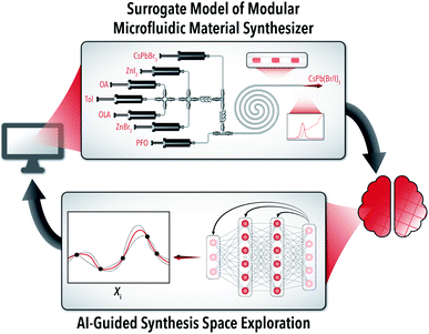
Given the nature of material synthesis space search algorithms under limited resources, the best possible theoretical methods can sometimes be beaten by random sampling within a given closed-loop experimental optimization campaign. The consistency in which an AI agent can search through a vast material synthesis space is, therefore, a more important algorithm metric than the outcome of a single optimization. However, in a physical experimentation platform, an impractically large number of experiments are required to determine the optimization variance for a large set of input parameters (≥5). In this work, we develop a simulation-optimization framework for evaluating AI algorithm performance within a single-period horizon RL setting. Single-period horizon refers to a myopic decision-making policy that maximizes expected reward through the consideration of reward/regret obtained from a single experimental decision. Here, reward/regret functions can measure information gained from the result of running an experiment but can also factor in the time to run such an experiment or the amount of material consumed. Surrogate modeling of experimentally obtained QD synthesis data using a robotic quantum dot synthesizer platform – shown in Fig. 1 – facilitated multiple material synthesis exploration campaigns. We selected lead halide perovskite (LHP) QDs as our testbed of AI-guided material synthesis exploration, due to their potential impact in next-generation display and photovoltaic devices.30–32
The surrogate model used in this study, built from over 1000 physically conducted experiments, replicates the experimentally derived failure rate of the microfluidic material synthesis platform, non-emitting sample regions, sampling variance for three output parameters, and predicted outputs. Using the developed AI-guided LHP QD synthesis framework within a high-performance computing environment, we conduct the equivalent of over 600![[thin space (1/6-em)]](https://www.rsc.org/images/entities/char_2009.gif) 000 experiments (normally requiring over 400 L of precursors and 7.5 years of continuous operation in a microfluidic reactor) to systematically study the performance of more than 150 AI-guided material space exploration strategies. We validate the accuracy of the developed surrogate model in replicating an experimental space with experimental optimization campaigns conducted using the developed autonomous QD synthesis bot. Then, we automatically investigate different aspects of RL-based LHP QD synthesis through tuning of the belief model architecture, AI-guided decision policies, and data boosting algorithms. The results of the optimized AI-guided material synthesis agent are then compared with four established optimization algorithms. With this optimized RL-based LHP QD synthesis approach, we demonstrate a mixed exploration/exploitation strategy for comprehensively studying the vast colloidal synthesis universe of LHP QDs in as few experiments as possible (i.e., minimum time and chemical resources).
000 experiments (normally requiring over 400 L of precursors and 7.5 years of continuous operation in a microfluidic reactor) to systematically study the performance of more than 150 AI-guided material space exploration strategies. We validate the accuracy of the developed surrogate model in replicating an experimental space with experimental optimization campaigns conducted using the developed autonomous QD synthesis bot. Then, we automatically investigate different aspects of RL-based LHP QD synthesis through tuning of the belief model architecture, AI-guided decision policies, and data boosting algorithms. The results of the optimized AI-guided material synthesis agent are then compared with four established optimization algorithms. With this optimized RL-based LHP QD synthesis approach, we demonstrate a mixed exploration/exploitation strategy for comprehensively studying the vast colloidal synthesis universe of LHP QDs in as few experiments as possible (i.e., minimum time and chemical resources).
All experiments presented in this work cover material exploration from a starting position of no prior knowledge. While many AI-guided experimentation methods implement prior knowledge or mechanistic models as initial estimates of the material space,22 the limited data availability, composition and morphological diversity, and high reaction sensitivity of many colloidal nanomaterials make informed material exploration difficult to conduct effectively.
Results and discussion
Experimental microfluidic LHP QD synthesis studies
The exemplary colloidal synthesis explored in this study is the halide exchange of cesium lead bromide QDs with zinc halide salts in a continuous modular microfluidic reactor. The microreactor is a custom modular system built from off-the-shelf commercial junctions and fluoropolymer capillary tubing (fluorinated ethylene propylene, FEP). Spectral sampling is conducted using a custom-built flow cell to accurately obtain photoluminescence and absorption spectra of the in-flow synthesized LHP QDs. The sampling space covers concentration ranges for five reactive components: starting LHP QDs (CsPbBr3), zinc iodide (ZnI2), oleic acid (OA), oleylamine (OLA), and zinc bromide (ZnBr2). While the relative concentration of each input stream can be varied individually, the total flow rate of the reactive phase in the microreactor is held constant through dilution with a toluene (Tol) stream, and the reactive phase is segmented into isolated droplets with a perfluorinated carrier oil (PFO). The development of this modular robotic platform is comprehensively reported in prior work.26,28,33 Utilizing the developed autonomous LHP QD synthesis bot (Fig. 1), we conducted over 1000 optimization experiments producing reliable in-house generated data for training and development of an accurate experimental system simulator (i.e., surrogate model).Surrogate model simulator
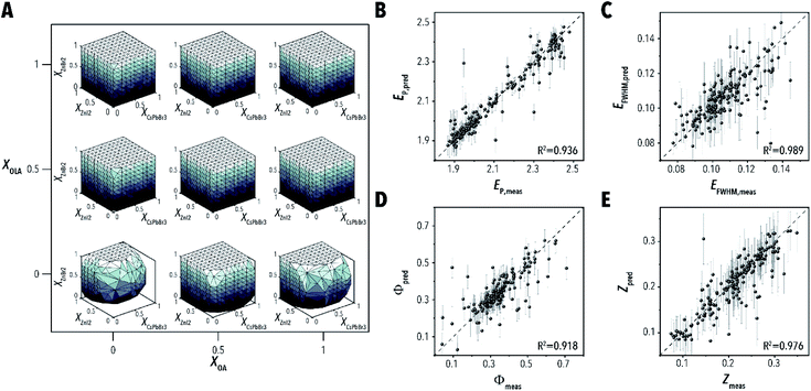
The surrogate model, illustrated in Fig. 2, is comprised of four experimentally validated functions. (i) The global failure rate is representative of the 1.5% probability of experiment failure, which results in no measurable output parameters. In a real-world closed-loop autonomous system, malfunctions in equipment or data processing algorithms are a regular occurrence that must be sufficiently addressed by an AI-guided material synthesis algorithm. Handling of these abnormalities are particularly important for the case study system as a failed experiment is indistinguishable from a valid experiment conducted in a non-emitting region of the sample space.Further building upon this distinction, (ii) the developed surrogate model checks whether the given input conditions are within a synthesizable region of the colloidal synthesis space, shown in Fig. 3A. Using a naïve Bayes classifier trained on the starting 1000 sample data set, the feasibility model predicts whether the provided input parameters (Xi) will produce an emitting solution of LHP QDs. Between experiment failure and unfeasible sampling regions, 4.5% of the training data set resulted in no measurable parameters. Given that the input parameters are projected to produce a viable experiment, (iii) the output of each parameter is predicted by sampling from a ground truth model comprised of three Gaussian process regressions (GPRs) corresponding to each of the three output parameters – peak emission energy (EP), emission full-width at half-maximum (EFWHM), and photoluminescence quantum yield (Φ).
The large data set sufficiently trained the ground truth model (i.e., LHP QD synthesis simulator) for accurate prediction of the output parameters as well as the quality metric objective functions (Z) for 200 test experiments, shown in Fig. 3B–E. Ensemble neural network (ENN) models were shown to be equally effective in prediction accuracy; however, GPs were chosen for the reduced computational requirements. Finally, (iv) to simulate the expected measurement variability, addition, homoscedastic Gaussian noise is applied to each of the output values as determined by the variance of each parameter (see ESI Section S.1‡ for more details). Using the developed multi-stage surrogate model of a real-world microfluidic material synthesis platform, the parameters and strategies surrounding AI-guided material synthesis algorithms can be extensively explored. The surrogate model was further compared to real-world experimental data sets through campaigns designed to mimic optimizations conducted in prior work. The optimizations, using the ENN model reported in prior literature, produced optimization algorithm performance windows that capture the real-world data effectively – see ESI section S.2.‡
Multi-objective optimization
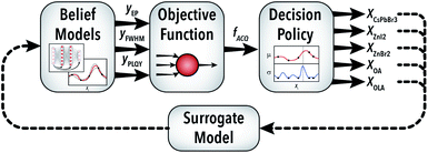
The first challenge in selecting an effective autonomous experimentation strategy for materials development with multiple outputs is identifying a method to simultaneously handle the target objectives. Illustrated in Fig. 4, the AI-guided material synthesis algorithm within a single-period horizon RL framework is comprised of a belief model, an objective function, and a decision policy. The objective function operates by converting the three output parameter predictions of the belief model into a single quality metric (Z), which the decision policy uses to select the next experimental conditions.In this work, we evaluate two objective function techniques: (i) a weighted mean utility function and (ii) probability sampling of the three output parameters. The utility form of the objective function (Zutil) is a weighted mean of the three outputs defined by percentage weights [APE, AFWHM, APLQY] after appropriate non-dimensionalization and inversion of the variables:
 | (1) |
Parameter sampling operates similarly; however, instead of applying these weights to the normalized output parameters, each parameter is individually optimized. At the time of experimentation, samples are allocated with a selection probability corresponding to [APE, AFWHM, APLQY], as shown by
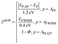 | (2) |
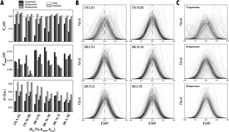
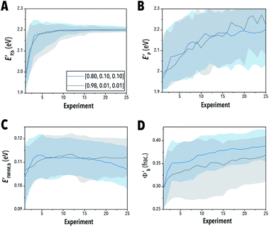
Using the above-mentioned multi-objective strategies with an expected improvement (EI) decision policy on a GP belief model (ESI Section S.3‡), seven sets of data weights were tested with 100 replicates for each LHP QD optimization campaign. As shown in Fig. 5A, objective function sampling outperformed probability sampling for most parameter weight sets, and, while selection of appropriate quality metrics across different output weight models is difficult to impose without bias, the weight set [0.8, 0.1, 0.1] appears to most holistically optimize the three LHP QD output parameters. The valuation of each parameter is ultimately a qualitative decision, and a comparison of the predicted optical spectra indicates that most of the tested data weights are sufficient optimization tools producing similar results (Fig. 5B). Upon closer inspection, however (Fig. 5A), the weight set [0.8, 0.1, 0.1] produced the highest precision EP after 20 experiments without sacrificing quality in EFWHM and Φ. As expected, the quality of the highest performing measurement consistently improves as the number of experiments increases and the best measured spectra across all replicates narrows onto an optimum (Fig. 5C).
Interestingly, the simulation results for the weight set [0.98, 0.1, 0.1], which should prioritize achieving an optimal EP value underperforms in terms of the best achieved EP value compared to a more balanced weight set [0.8, 0.1, 0.1] (Fig. 6A and B). This observed behavior points to a training regularization effect of running experiments not specifically geared toward achieving a single objective. By focusing only on EP values, the EI policy tended to not as effectively explore the accessible LHP QD synthesis space in order to discover potentially better regions for EP, and this haste by EI to exploit rather than explore is mitigated when opting for a multi-target optimization. This undesirable behavior of EI has been previously reported.34 For example, Gongora et al.35 suggests a random discretization of design space as a preprocessing step prior to calculating EI values to prevent early exploitation. With respect to EFWHM and Φ, the balanced weight sets allowed for notable improvements over the EP biased weighting, as expected. Furthermore, the balanced weight set was able to improve the FWHM and PLQY significantly over the biased weight experiments (Fig. 6C and D).
Ensemble neural network design
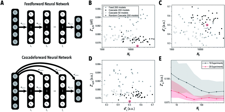
After building an understanding of experiment selection algorithm performance under various multi-parameter handling strategies, the next aim was to develop an effective ENN-based belief modeling algorithm.36 Ensemble modeling strategies in contrast to GPR models, implement a collection of models – each of which is individually unlikely to comprehensively represent the chemical synthesis space – and combines them into a single effective predictor. The ensemble models used in this work were feed and cascade forward, dense neural networks (NNs) – shown in Fig. 7A.Individual NNs fi(x) can be trained to obtain predictions of an experimental response given some set of experimental inputs x. Associated with each model within the ensemble is a weight, θi, which represents the posterior probability that model fi describes the ground-truth function generating the data. Through combination of these NNs and their weight terms into the ensemble, we can obtain estimates of the response and corresponding uncertainty
 | (3) |
 | (4) |
 | (5) |
Such estimates, uncertainties, and covariances are then used in subsequent decision-making policies to calculate expected rewards/regret for running a particular experiment. While other types of neural networks are appropriate for high-dimensional structured input data, such as convolutional neural networks for image data,37,38 or for sequential data, such as long short-term memory networks,39,40 in the case of solution-processed materials, the input data is neither high-dimensional nor structured. As such, we treat the five-dimensional LHP QD synthesis parameters directly as input features to a dense NN.
Next, we systematically varied the architecture of the neural networks within the ENN model from one to six layers with one to five nodes per layer – further detailed in ESI Section S.4.‡ In addition to this strategy, different combinations of constraints were employed on a set of randomly selected architectures where each model in the ensemble featured a different combination of nodes and layers, as shown in Table 1.
| Variant | N L | N N |
|---|---|---|
| A | 1 to 6 | 1 to 5 |
| B | 1 to 6 | 1 to 3 |
| C | 1 to 6 | 2 |
| D | 2 to 4 | 1 to 5 |
| E | 2 to 4 | 1 to 3 |
| F | 2 to 4 | 2 |
| G | 3 | 1 to 5 |
| H | 3 | 1 to 3 |
After training an ENN model on acquired data sets, an EI decision policy was used to search the generated LHP QD synthesis model for the next experiment to conduct. The quality of the optimization was evaluated by fitting the median best measured objective function  value from 100 optimization replicates to a learning rate decay curve to attain the learning rate decay
 | (6) |
Z
b(ie) is the best measured objective function value as a function of the experiment number, η0 is the initial learning rate, ie is the experiment number, and Z∞ is the predicted convergent objective function value as ie → ∞. Additionally, the median best measured objective function value after 25 experiments  was compared across the tested models.
Throughout the ENN-based optimization campaigns, the cascade forward structure consistently outperformed feed forward neural networks. For both equivalent architecture and total parameters – see ESI Section S.5‡ – cascade forward-based ENNs resulted in lower  and higher
  than corresponding feed forward ENNs (Fig. 7B–D). It should be noted that this advantage is present while using typical training parameters. Under an alternative training algorithm, feed forward ENNs could significantly improve in performance, even beyond the capabilities of cascade forward ENNs. While many of the randomized neural network architecture ENNs performed similarly to the constant structure ENNs, the ENN architecture variant F (i.e., two to four layers with two nodes per layer) was able to reach the lowest median
  with a moderately high
  Furthermore, increasing the size of the ensembles from 50 to 200 models (Fig. 7B) improved model performance notably across all architectures. Shown in Fig. 7E, based on the behavior of this highest performing ENN architecture, the improvements were unlikely to continue past 200 models. While the number of models in the ensemble may be reduced to lower computational costs at the expense of precision, ensembles greater than 200 models do not provide any clear additional benefit.
Decision policies
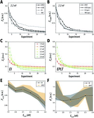
Decision policies are the algorithms used to intelligently select of the next experimental condition based on the predictions and uncertainty of a given model. A simplistic optimization algorithm will select experimental conditions at the predicted optimum of the model, also known as pure exploitation (EPLT). However, in scarce data availability scenarios, this technique is often inefficient as large regions of the accessible synthesis space are left underexplored. Alternatively, the decision policy may respond to the model uncertainty – e.g., the variance across models in an ensemble for a given input – and select experiments where the greatest information may be attained, also known as maximum variance (MV). Furthermore, comprehensively understanding a material synthesis space is also inefficient for extracting a single set of optimal input conditions for a given optimization campaign. The best decision policies take into consideration both exploitation of the predicted optima and exploration of the accessible material synthesis space. In this work, two common mixed exploration-exploitation decision policies were studied, upper confidence bound (UCB) and EI.Shown in Fig. 8A, both EI and UCB reached a lower  than MV and EPLT throughout the entirety of the optimization. MV is not expected to sample the optimal formulation, but it is reasonable to expect the policy to build an accurate belief model. However, when the ENNs built through each policy were instructed to predict the optimal conditions after each experiment (Fig. 8B), EI and UCB still produced lower median objective function values
  than both MV and EPLT. While UCB and EI resulted in very similar learning curves, the UCB policy presented here is the result of tuning the explore-exploit control parameter (ε) over twelve campaigns – see ESI Section S.6.‡ EI inherently does not require this same tuning and is therefore considered the more favorable decision policy for use in the AI-guided LHP QD synthesis.
Furthermore, the advantage of EI over EPLT demonstrates the necessity of partially exploratory policies over purely exploiting a belief model. This advantage is relatively small for the 2.2 eV target emission used in this study; however, expanding the number of target emissions (Fig. 8C and D) further demonstrates the superiority of EI. Throughout the entirety of the tunable parameter space, EI results in lower  than EPLT and can reach these values more consistently (Fig. 8E and F). This advantage is most apparent near the outer bounds of the attainable synthesis space – i.e. at an Ep of 1.9 eV and 2.4 eV. Exploitation of the model can likely capture parameters near the optima, but due to the challenges of extrapolation outside the understood reaction space, more complex strategies that attempt to first explore that external space are required when optimizing near the system extremes.
Performance comparisons
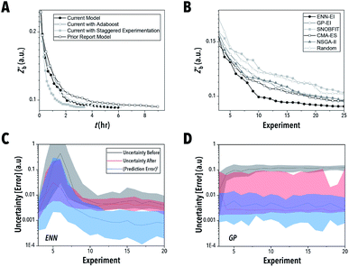
Recently, our group has demonstrated the application of ENN modeling36 in real-time, AI-guided QD synthesis.28 While the efficacy of AI methods for accelerated formulation discovery and synthesis optimization of colloidal LHP QDs was demonstrated, the large data requirements make fine tuning of these parameters unrealistic to attain experimentally. Additionally, the advantages of such ENN algorithms over conventional GPR-based and other established methods such as the Non-dominated Sorting Genetic Algorithm II (NSGA-II)41–43 or Covariance Matrix Adaption-Evolutionary Strategy (CMA-ES)42 remain unclear due to the inherent variability in simple optimization performance for uninformed chemical synthesis studies.Shown in Fig. 9A, the newly developed ENN-EI structure provides clear advantages over the prior reported structure in both computational cost and optimization efficiency and effectiveness. Furthermore, the inclusion of the ensemble boosting algorithm Adaboost.RT44,45 produced no clear advantage over the standard ENN which uses a uniform weighted mean within the ensemble. Finally, the effect of staggering the experiment execution and synthesis formulation selection was evaluated. Staggered sampling, as reported in our prior work, allows the optimization algorithm to search for the next experimental conditions while the robotic material synthesizer is operating, therefore maximizing the available time of the experimental platform. This process is conducted by providing experiments 1 to ie − 1 to the AI-guided synthesis algorithm while sample ie is being collected. This process reduces the total optimization time and, as demonstrated by the simulation campaigns, does not significantly reduce the effectiveness of the AI-guided synthesis algorithm.
In the next set of simulation campaigns, we investigated the performance of the optimized ENN-EI algorithm vs. established optimization algorithms. The newly tuned ENN-based autonomous material synthesis method provided a clear advantage over all tested established optimization techniques (Fig. 9B). Even though both evolutionary strategies, CMA-ES and NSGA-II, were pre-tuned for their generation population size (ESI Section S.7‡), neither matched the performance of ENN-EI. Additionally, SNOBFIT performed similarly to a pure exploration policy, a finding similar to our prior reported work. It should be noted that at higher experiment numbers, SNOBFIT is expected to converge onto an optima, while pure exploration is most likely to fail. In comparing the highest performing AI-guided synthesis strategies, the ENN method demonstrated a clear advantage over GP – shown in Fig. 9B–D.
To better understand the performance improvement of ENN models over GPs, the marginal impact of an additional data point after every experiment was studied. As shown in Fig. 9C and D, the uncertainties associated with the experimental response before and after the experiment is run (gray and red lines) are closer to one another when using an ENN model than they are when using GP. This suggests that GPs (at least with a squared-exponential kernel) learn locally – a single data point describing the experimental response at some input x provides significant correlative information for the experimental responses x′ nearby. In contrast, in the ENN, the information provided by a single data point impacts the entire training of the ensemble models, especially in the case of low data. The correlation between prediction error and model uncertainty may be further understood using the Kendall rank coefficient. By comparing the median uncertainty before sampling and prediction error (shown in Fig. 9C–D) through a one-sided Kendall tau test, the ENN resulted in a p-value of <0.01, indicating that there is a correlation between the uncertainty and error, while the GP resulted in a p-value of 0.61, which failed to identify a correlation.
As a result, a single data point may impact the prediction being made globally. This is not unlike the effect seen when training a parametric model – a change in parameter values impacts the predictions made by such model for any choice of inputs to that model. Therefore, the ENN updates models globally while the GP updates them locally. This effect may be exaggerated particularly in the case of the EI policy, which has been demonstrated to stagnate due an eventual imbalance between exploration and exploitation. Because uncertainties are not decreased in a local manner with ENN, such a stagnation may be mitigated, allowing for a more exploratory search to take place with ENN-EI versus GP-EI.
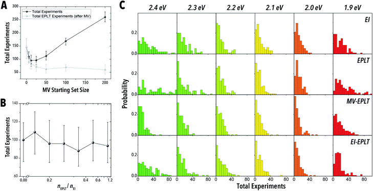
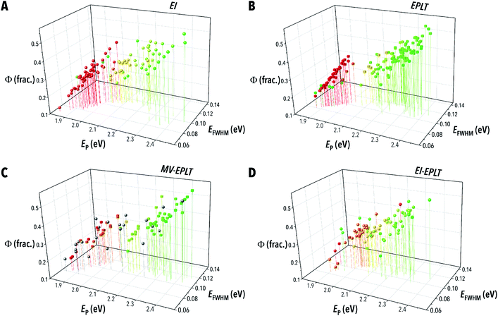
As shown in Fig. 10C and Fig. 11A–D, the policies reliant on EPLT consistently struggle to reach the stopping criteria at the outer bounds of the LHP QD synthesis space, a finding similar to that shown in the uninformed studies. Even with a prior training set (MV-EPLT), EPLT struggles to find these outer bound optima, which suggests that MV on its own does not completely capture the full range of relevant colloidal synthesis conditions in the number of experiments allotted. In the internal positions of the material synthesis space, i.e., setpoints 2.0 eV to 2.3 eV, EPLT performs similarly to EI. However, EI-EPLT provided the most efficient navigation of the LHP QD synthesis space. This meta-decision policy operates efficiently due to the targeted exploration of the outer bounds of the material synthesis space through EI, followed by the exploitation of the newly structure model through an EPLT policy.
Meta-decision policy analysis
While typical examples of one-off campaigns (such as Bayesian optimization) prioritize balanced exploration and exploitation within a campaign, we may consider a broader class of meta-decisions to be made when planning and coordinating between several optimization campaigns, which is consistent to how experiments are run and how science advances in general. For example, we may consider a meta policy that learns generic information about a material synthesis space prior to any optimization campaign, especially when seeking multiple optimized products from the same synthesis space (e.g., LHP QDs with different emission colors from the same batch of starting precursors). This generic, learned prior information could then be used in optimization campaigns over which the initial up-front costs of learning are amortized. We can then consider the optimal trade-off between general, global learning and optimization in terms of the total amount of time needed to perform both types of campaigns together for multiple targeted output materials. Such cost-based, episodic methods could be explicitly modeled and optimized using episodic RL techniques, but here we shall perform a simulation-based study to similarly identify the optimal balance.Four types of meta-decision policies were evaluated through multi-stage optimization completion criteria. The optimizations were performed by consecutively targeting peak emissions of 1.9–2.4 eV using 0.1 eV intervals and additive data across the set-points. The stopping criteria were met when, at each set point, the measured peak emission was within 2 meV of the target peak emission energy. The MV-EPLT policy was conducted by first sampling a starting set size of MV selected experiments, followed by EPLT for each of the target emissions (Fig. 10A). The EI-EPLT policy operated by performing consecutive EI experiments followed by a single EPLT selected experiment. The obtained ratio of EPLT to EI experiments (nEPLT/nEI) for each optimization campaign is shown in Fig. 10B. We also conducted pure EPLT and pure EI as control experiments. As shown in Fig. 10A and B, an MV starting set size of 12–25 experiments passed the stopping criteria in the shortest number of experiments for the MV-EPLT policy, but the EI-EPLT policy at a ratio of 0.25 outperformed MV-EPLT by 8 experiments.
It should be noted that while the use of a surrogate model has enabled further development of a range of experiment selection algorithms, there are limitations to surrogate representations of real-world systems. Most notably, the ground truth model surface is likely smoother than the actual system, resulting in more optimistic estimates of the selection algorithm effectiveness. In this case, the performance of ENN methods in the surrogate model will likely be boosted over a real-world system. However, based on the comparison of real-world optimization runs with the surrogate system (ESI Section S.2‡), the developed surrogate model appears to approximately reflect the expected performance of the tested algorithms. Furthermore, the comparison of the proposed optimal ENN algorithm with various ENN variants as well as with established algorithms is intended to demonstrate the effectiveness of the methods and not necessarily claim a holistic advantage.
Conclusions
In this work, 600![[thin space (1/6-em)]](https://www.rsc.org/images/entities/char_2009.gif) 000 simulated autonomous materials development experiments were conducted using a single-period horizon RL algorithm integrated with a multi-stage surrogate material synthesis model derived from 1000 real-world experiments implementing an autonomous microfluidic reactor. More than 150 different AI-guided material space exploration algorithms with tuneable meta-decisions were evaluated in their ability to effectively optimize quality metrics of LHP QDs (i.e., quantum yield and emission linewidth) at a target emission energy via halide exchange reactions. Through this work, an AI-guided materials development algorithm from the position of no prior knowledge was automatically developed (Auto-AI)—unattainable through real-world experimental trial and error strategies—by systematic investigation of the multi-objective handling methods, model architectures, meta-decisions, and decision policies. The developed ENN-based materials development algorithm outperformed previously established material space exploration strategies and achieved a significant increase in optimization precision over GPR-based algorithms. Furthermore, a comprehensive strategy for exploring a multi-target output space was developed and characterized, enabling rapid exploration of new material spaces featuring tunable parameters such as peak emission. Further implementation of the ENN-based Auto-AI models and methods presented in this work will facilitate the adoption of autonomous robotic experimentation strategies for discovery and formulation optimization of emerging energy-relevant materials.
000 simulated autonomous materials development experiments were conducted using a single-period horizon RL algorithm integrated with a multi-stage surrogate material synthesis model derived from 1000 real-world experiments implementing an autonomous microfluidic reactor. More than 150 different AI-guided material space exploration algorithms with tuneable meta-decisions were evaluated in their ability to effectively optimize quality metrics of LHP QDs (i.e., quantum yield and emission linewidth) at a target emission energy via halide exchange reactions. Through this work, an AI-guided materials development algorithm from the position of no prior knowledge was automatically developed (Auto-AI)—unattainable through real-world experimental trial and error strategies—by systematic investigation of the multi-objective handling methods, model architectures, meta-decisions, and decision policies. The developed ENN-based materials development algorithm outperformed previously established material space exploration strategies and achieved a significant increase in optimization precision over GPR-based algorithms. Furthermore, a comprehensive strategy for exploring a multi-target output space was developed and characterized, enabling rapid exploration of new material spaces featuring tunable parameters such as peak emission. Further implementation of the ENN-based Auto-AI models and methods presented in this work will facilitate the adoption of autonomous robotic experimentation strategies for discovery and formulation optimization of emerging energy-relevant materials.
Author contributions
Conceptualization R. W. E., K. G. R., M. A.; data curation R. W. E.; formal analysis R. W. E., A. A. V.; funding acquisition M. A.; investigation R. W. E, K. G. R., M. A.; methodology R. W. E., K. G. R., M. A.; project administration M. A.; software R. W. E, K. G. R.; validation R. W. E. (lead), A. A. V.; writing – original draft preparation R. W. E., A. A. V., K. G. R., M. A.; writing – review and editing R. W. E., A. A. V., M. A.Conflicts of interest
There are no conflicts to declare.Acknowledgements
The authors gratefully acknowledge the financial support provided by the National Science Foundation (Award # 1902702 and 1936527), the UNC Research Opportunities Initiative (UNC-ROI) Grant, and North Carolina State University. We acknowledge the computing resources provided on Henry2, a high-performance computing cluster operated by North Carolina State University. We also thank Dr Jianwei Dian and Dr Lisa L. Lowe for their assistance with parallelization and resource allocation, which was provided through the Office of Information Technology HPC services at NCSU.References
- J. Li, K. Lim, H. Yang, Z. Ren, S. Raghavan, P.-Y. Y. Chen, T. Buonassisi and X. Wang, Matter, 2020, 3, 393–432 CrossRef.
- Q. A. Akkerman, G. Rainò, M. V Kovalenko and L. Manna, Nat. Mater., 2018, 17, 394 CrossRef CAS PubMed.
- A. Vikram, V. Kumar, U. Ramesh, K. Balakrishnan, N. Oh, K. Deshpande, T. Ewers, P. Trefonas, M. Shim and P. J. A. Kenis, ChemNanoMat, 2018, 4, 943–953 CrossRef CAS.
- A. M. Nightingale and J. C. de Mello, J. Mater. Chem., 2010, 20, 8454–8463 RSC.
- N. Sitapure, R. Epps, M. Abolhasani and J. S.-I. Kwon, Chem. Eng. J., 2020, 127905 Search PubMed.
- L. Porwol, D. J. Kowalski, A. Henson, D. Long, N. L. Bell and L. Cronin, Angew. Chem., Int. Ed., 2020, 59, 11256–11261 CrossRef CAS PubMed.
- P. S. Gromski, A. B. Henson, J. M. Granda and L. Cronin, Nat. Rev. Chem., 2019, 3, 119–128 CrossRef.
- S. Langner, F. Häse, J. D. Perea, T. Stubhan, J. Hauch, L. M. Roch, T. Heumueller, A. Aspuru-Guzik and C. J. Brabec, Adv. Mater., 2020, 32, 1907801 CrossRef CAS PubMed.
- J. P. Correa-Baena, K. Hippalgaonkar, J. van Duren, S. Jaffer, V. R. Chandrasekhar, V. Stevanovic, C. Wadia, S. Guha and T. Buonassisi, Joule, 2018, 2, 1410–1420 CrossRef CAS.
- N. T. P. Hartono, J. Thapa, A. Tiihonen, F. Oviedo, C. Batali, J. J. Yoo, Z. Liu, R. Li, D. F. Marrón, M. G. Bawendi, D. Fuertes Marrón, M. G. Bawendi, T. Buonassisi and S. Sun, Nat. Commun., 2020, 11, 1–9 Search PubMed.
- R. Gómez-Bombarelli, J. N. Wei, D. Duvenaud, J. M. Hernández-Lobato, B. Sánchez-Lengeling, D. Sheberla, J. Aguilera-Iparraguirre, T. D. Hirzel, R. P. Adams and A. Aspuru-Guzik, ACS Cent. Sci., 2018, 4, 268–276 CrossRef PubMed.
- Z. Li, M. A. Najeeb, L. Alves, A. Z. Sherman, V. Shekar, P. Cruz Parrilla, I. M. Pendleton, W. Wang, P. W. Nega, M. Zeller, J. Schrier, A. J. Norquist and E. M. Chan, Chem. Mater., 2020, 32, 5650–5663 CrossRef CAS.
- D. Salley, G. Keenan, J. Grizou, A. Sharma, S. Martín and L. Cronin, Nat. Commun., 2020, 11, 2771 CrossRef CAS PubMed.
- K. M. Jablonka, D. Ongari, S. M. Moosavi and B. Smit, Big-Data Science in Porous Materials: Materials Genomics and Machine Learning, 2020, vol. 120 Search PubMed.
- F. Mekki-Berrada, Z. Ren, T. Huang, W. K. Wong, F. Zheng, J. Xie, I. P. S. Tian, S. Jayavelu, Z. Mahfoud, D. Bash, K. Hippalgaonkar, S. Khan, T. Buonassisi, Q. Li and X. Wang, ChemRxiv, 2020, DOI:10.26434/CHEMRXIV.12673742.V1.
- D. P. Tabor, L. M. Roch, S. K. Saikin, C. Kreisbeck, D. Sheberla, J. H. Montoya, S. Dwaraknath, M. Aykol, C. Ortiz, H. Tribukait, C. Amador-Bedolla, C. J. Brabec, B. Maruyama, K. A. Persson and A. Aspuru-Guzik, Nat. Rev. Mater., 2018, 3, 5–20 CrossRef CAS.
- A. A. Volk, R. W. Epps and M. Abolhasani, Adv. Mater., 2021, 33, 2004495 CrossRef CAS PubMed.
- K. Abdel-Latif, R. W. Epps, F. Bateni, S. Han, K. G. Reyes and M. Abolhasani, Adv. Intell. Syst., 2020, 2000245 Search PubMed.
- Z. S. Campbell, F. Bateni, A. A. Volk, K. Abdel-Latif and M. Abolhasani, Part. Part. Syst. Charact., 2020, 37, 2000256 CrossRef CAS.
- K. Abdel-Latif, F. Bateni, S. Crouse and M. Abolhasani, Matter, 2020, 3, 1053–1086 CrossRef.
- S. Krishnadasan, R. J. C. Brown, A. J. deMello and J. C. deMello, Lab Chip, 2007, 7, 1434–1441 RSC.
- C. W. Coley, D. A. Thomas, J. A. M. Lummiss, J. N. Jaworski, C. P. Breen, V. Schultz, T. Hart, J. S. Fishman, L. Rogers, H. Gao, R. W. Hicklin, P. P. Plehiers, J. Byington, J. S. Piotti, W. H. Green, A. J. Hart, T. F. Jamison and K. F. Jensen, Science, 2019, 365, eaax1566 CrossRef CAS PubMed.
- S. Steiner, J. Wolf, S. Glatzel, A. Andreou, J. M. Granda, G. Keenan, T. Hinkley, G. Aragon-Camarasa, P. J. Kitson, D. Angelone and L. Cronin, Science, 2019, 363, eaav2211 CrossRef CAS PubMed.
- L. Bezinge, R. M. Maceiczyk, I. Lignos, M. V Kovalenko and A. J. deMello, ACS Appl. Mater. Interfaces, 2018, 10, 18869–18878 CrossRef CAS PubMed.
- R. M. Maceiczyk and A. J. Demello, J. Phys. Chem. C, 2014, 118, 20026–20033 CrossRef CAS.
- R. W. Epps, A. A. Volk, K. Abdel-Latif and M. Abolhasani, React. Chem. Eng., 2020, 5, 1212–1217 RSC.
- J. Li, J. Li, R. Liu, Y. Tu, Y. Li, J. Cheng, T. He and X. Zhu, Nat. Commun., 2020, 11, 2046 CrossRef CAS PubMed.
- R. W. Epps, M. S. Bowen, A. A. Volk, K. Abdel-Latif, S. Han, K. G. Reyes, A. Amassian and M. Abolhasani, Adv. Mater., 2020, 2001626 CrossRef CAS PubMed.
- W. Huyer and A. Neumaier, ACM Trans. Math. Software, 2008, 35, 9 CrossRef.
- E. H. Sargent, Nat. Photonics, 2012, 6, 133–135 CrossRef CAS.
- K. S. Cho, E. K. Lee, W. J. Joo, E. Jang, T. H. Kim, S. J. Lee, S. J. Kwon, J. Y. Han, B. K. Kim, B. L. Choi and J. M. Kim, Nat. Photonics, 2009, 3, 341–345 CrossRef CAS.
- S. Wang, Y. Wang, Y. Zhang, X. Zhang, X. Shen, X. Zhuang, P. Lu, W. W. Yu, S. V. Kershaw and A. L. Rogach, J. Phys. Chem. Lett., 2019, 10, 90–96 CrossRef CAS PubMed.
- K. Abdel-Latif, R. W. Epps, C. B. Kerr, C. M. Papa, F. N. Castellano and M. Abolhasani, Adv. Funct. Mater., 2019, 29, 1–13 Search PubMed.
- I. O. Ryzhov, On the convergence rates of expected improvement methods, 2015 Search PubMed.
- A. E. Gongora, B. Xu, W. Perry, C. Okoye, P. Riley, K. G. Reyes, E. F. Morgan and K. A. Brown, Sci. Adv., 2020, 6, eaaz1708 CrossRef PubMed.
- Y. Orimoto, K. Watanabe, K. Yamashita, M. Uehara, H. Nakamura, T. Furuya and H. Maeda, J. Phys. Chem. C, 2012, 116, 17885–17896 CrossRef CAS.
- Y. LeCun, L. Bottou, Y. Bengio and P. Haffner, Proc. IEEE, 1998, 86, 2278–2323 CrossRef.
- A. Krizhevsky, I. Sutskever and G. E. Hinton, ImageNet Classification with Deep Convolutional Neural Networks, 2012 Search PubMed.
- F. A. Gers, N. N. Schraudolph and J. Schmidhuber, Learning Precise Timing with LSTM Recurrent Networks, 2002, vol. 3 Search PubMed.
- H. Sak, A. Senior and F. Beaufays, arXiv, 2014, https://arxiv.org/abs/1402.1128 Search PubMed.
- K. Deb, A. Pratap, S. Agarwal and T. Meyarivan, IEEE Trans. Evol. Comput., 2002, 6, 182–197 CrossRef.
- C. Igel, N. Hansen and S. Roth, Evol. Comput., 2007, 15, 1–28 CrossRef PubMed.
- K. F. Koledina, S. N. Koledin, A. P. Karpenko, I. M. Gubaydullin and M. K. Vovdenko, J. Math. Chem., 2019, 57, 484–493 CrossRef CAS.
- Y. Freund and R. E. Schapire, Journal of Japanese Society for Artificial Intelligence, 1999, 14, 771–780 Search PubMed.
- D. P. Solomatine and D. L. Shrestha, in IEEE International Conference on Neural Networks - Conference Proceedings, 2004, vol. 2, pp. 1163–1168 Search PubMed.
Footnotes |
| † The surrogate model used to generate the data in this study is publicly available for download at https://github.com/AbolhasaniLab/Reaction-Optimization-Surrogate-Model. |
| ‡ Electronic supplementary information (ESI) available: Surrogate model design and validation, Gaussian process regression training parameters, ensemble neural net architecture and tuning, UCB parameter tuning, and evolutionary algorithm tuning. See DOI: 10.1039/d0sc06463g |
| This journal is © The Royal Society of Chemistry 2021 |

