 Open Access Article
Automatic discovery of photoisomerization mechanisms with nanosecond machine learning photodynamics simulations†
Jingbai
Li
a,
Patrick
Reiser
b,
Benjamin R.
Boswell
d,
André
Eberhard
c,
Noah Z.
Burns
 *d,
Pascal
Friederich
*bc and
Steven A.
Lopez
 *a
*a
aDepartment of Chemistry and Chemical Biology, Northeastern University, Boston, MA 02115, USA. E-mail: s.lopez@northeastern.edu
bInstitute of Nanotechnology, Karlsruhe Institute of Technology, Karlsruhe, Germany. E-mail: pascal.friederich@kit.edu
cInstitute of Theoretical Informatics, Karlsruhe Institute of Technology, Karlsruhe, Germany
dDepartment of Chemistry, Stanford University, Stanford, CA, USA. E-mail: nburns@stanford.edu
First published on 10th March 2021
Abstract
Photochemical reactions are widely used by academic and industrial researchers to construct complex molecular architectures via mechanisms that often require harsh reaction conditions. Photodynamics simulations provide time-resolved snapshots of molecular excited-state structures required to understand and predict reactivities and chemoselectivities. Molecular excited-states are often nearly degenerate and require computationally intensive multiconfigurational quantum mechanical methods, especially at conical intersections. Non-adiabatic molecular dynamics require thousands of these computations per trajectory, which limits simulations to ∼1 picosecond for most organic photochemical reactions. Westermayr et al. recently introduced a neural-network-based method to accelerate the predictions of electronic properties and pushed the simulation limit to 1 ns for the model system, methylenimmonium cation (CH2NH2+). We have adapted this methodology to develop the Python-based, Python Rapid Artificial Intelligence Ab Initio Molecular Dynamics (PyRAI2MD) software for the cis–trans isomerization of trans-hexafluoro-2-butene and the 4π-electrocyclic ring-closing of a norbornyl hexacyclodiene. We performed a 10 ns simulation for trans-hexafluoro-2-butene in just 2 days. The same simulation would take approximately 58 years with traditional multiconfigurational photodynamics simulations. We generated training data by combining Wigner sampling, geometrical interpolations, and short-time quantum chemical trajectories to adaptively sample sparse data regions along reaction coordinates. The final data set of the cis–trans isomerization and the 4π-electrocyclic ring-closing model has 6207 and 6267 data points, respectively. The training errors in energy using feedforward neural networks achieved chemical accuracy (0.023–0.032 eV). The neural network photodynamics simulations of trans-hexafluoro-2-butene agree with the quantum chemical calculations showing the formation of the cis-product and reactive carbene intermediate. The neural network trajectories of the norbornyl cyclohexadiene corroborate the low-yielding syn-product, which was absent in the quantum chemical trajectories, and revealed subsequent thermal reactions in 1 ns.
1. Introduction
Photochemistry provides access to highly strained molecular architectures,1 photoswitches,2 organic photovoltaics,3 and solar fuel materials,4,5 which are characterized by mild conditions and high atom economy. Photochemical reactions typically consist of a series of molecular transformations that occur in excited molecules after light absorption. Unlike ground state processes, where spectroscopy and crystallography reveal structural information, light-promoted excited-state reactions involve short-lived femto-to picosecond (10−15 to 10−12 s) molecular excited states and reactive intermediates. This ultrafast processes involve relaxation to the excited-state minima for fluorescence or non-radiative transition to the ground-state through a state crossing point or seam, which plays essential roles in the chemoselectivity of a photochemical reaction.6,7Unravelling the origin of chemoselectivity and stereoselectivity in organic photochemical reactions is challenging because of the short-lived molecular excited states. Quantum chemical calculations offer insight into the bonding changes that occur along a reaction coordinate and non-adiabatic molecular dynamics (NAMD) simulations to gain mechanistic insights and develop structure–reactivity relationships in complex photochemical reactions. The nuclei-electron coupling and time-dependent terms increase the complexity of Hamiltonian in NAMD and, thus, computation time. Multiple methods developed in the last two decades simplified the time-dependent molecular wave functions, e.g. ab initio multiple spawning (AIMS),8,9 and fewest switches surface hopping (FSSH).10–12 However, computing high dimensional PESs with the requisite multiconfigurational methods is extremely resource-intensive. For example, most quantum chemical software packages encode an upper limit to active space of 16 electrons and 16 orbitals for complete active space self-consistent field (CASSCF) calculations. A typical NAMD experiment requires thousands of such calculations, resulting in a maximum simulation time on the order of 1 picosecond, at a computational cost of approximately 101–104 wall-clock hours. Unfortunately, many direct excitation photochemical reactions have low quantum yields and long excited-state lifetimes. This results in prohibitively expensive NAMD simulations, thus limiting broad understanding of excited-state structure–reactivity relationships in photochemistry.
An increasing number of studies reported that fitting machine learning (ML) potentials could substantially accelerate the NAMD simulation.13–15 Aleotti et al. have parameterized ad hoc force fields for a 10 ps dynamic simulation of azobenzene.16 Westermeyr et al. have trained multilayer feedforward neural networks (NNs) to enable 1 ns simulation of methylenimmonium cation (CH2NH2+) in 59 days.17 Later, they have extended the application of the NN model in predicting excited-states electronic properties for other small molecules, such as SO2 and CSH2 employing a deep continuous-filter convolutional-layer neural network, SchNet, combined with SHARC.18 Recently, Ha et al. have trained the SchNet model to study the excited-state dynamics of penta-2,4-dieniminium cation.19 Applying ML-based NAMD on complex molecules continues to challenge theorists because of additional conformational flexibility and increase in available degrees of freedom. Training ML models becomes increasingly difficult with the rapidly growing required size of training datasets, especially when based on atom-wise molecular representations.
Here, we address the need for our combined ML and NAMD approach (ML-NAMD) that expands the scope of organic photochemical reactions. We demonstrate the high accuracy in the trained NN and low computational cost in the ML-NAMD simulations. Our trajectory statistics support that the ML-NAMD predicted photochemical product distribution is in good agreement with quantum chemical results. Our initial ML-NAMD simulations focused on the first such photodynamics of hexafluoro-2-butene (1), which is mechanistically well understood due to its characteristic vertical ππ* excitation from HOMO to LUMO (the π and π*-orbital). Hexafluoro-2-butene is a nontoxic and not flammable industrial working fluid used as a refrigerant and a foam-blowing agent.20 We also applied the ML-NAMD simulations to the 4π-electrocyclic ring-closing of norbornyl cyclohexadiene (3), a previously unknown and complex photochemical system.
2. Computational methods
2.1 Quantum chemical calculations
We performed quantum chemical calculations with OpenMolcas 19.11![[thin space (1/6-em)]](https://www.rsc.org/images/entities/char_2009.gif) 21 to generate reference and training data. We chose the less resource-intensive CASSCF method because it produced consistent potential energy surfaces with CASPT2 calculations, tested by the interpolated reaction coordinate diagrams of the model reactions (Fig. S11 and S17†). The converged orbitals and optimized geometries are available in the ESI.†
21 to generate reference and training data. We chose the less resource-intensive CASSCF method because it produced consistent potential energy surfaces with CASPT2 calculations, tested by the interpolated reaction coordinate diagrams of the model reactions (Fig. S11 and S17†). The converged orbitals and optimized geometries are available in the ESI.†
In the cis–trans isomerization of trans-1, we selected an active space of 2 π-electrons and 2 π-type orbitals (i.e. (2,2)) for the C![[double bond, length as m-dash]](https://www.rsc.org/images/entities/char_e001.gif) C bond. The geometries of trans-1 and cis-1 were optimized with the cc-pVDZ basis set.22 A vibrational analysis confirmed only positive frequencies. We located two minimum energy crossing points (MECPs) corresponding to the trans → cis (MECP-trans-1) and the reverse reaction (MECP-cis-1). The NAMD simulations with CASSCF(2,2)/cc-pVDZ used the fewest switches surface hopping algorithm (FSSH)10–12 in Hammes-Schiffer/Tully (HST) scheme10 with decoherence correction of 0.1 Hartree23 implemented in OpenMolcas 19.11.21 We generated 1500 initial geometries and associated velocities near the equilibrium geometry of trans-1 with Wigner sampling at 300 K. The NAMD trajectories were propagated at 300 K (Nosé–Hoover thermostat24) from the S1 Franck–Condon region for ∼500 fs with 0.5 fs timesteps. It is important to note that applying a thermostat can bias the excited-state dynamics because the excited-state lifetime of a few hundred femtoseconds often does not suffice for thermalization. We used a thermostat to reduce the kinetic energy gained from surface hopping, which compensates for the overestimated excitation energy of CASSCF calculation. We collected 1371 of the 1500 trajectories that reached the ground-state within 500 fs, whereas the others remained in the excited-state or showed molecular structures with unexpected broken bonds resulting from incorrectly converged CASSCF calculations.
C bond. The geometries of trans-1 and cis-1 were optimized with the cc-pVDZ basis set.22 A vibrational analysis confirmed only positive frequencies. We located two minimum energy crossing points (MECPs) corresponding to the trans → cis (MECP-trans-1) and the reverse reaction (MECP-cis-1). The NAMD simulations with CASSCF(2,2)/cc-pVDZ used the fewest switches surface hopping algorithm (FSSH)10–12 in Hammes-Schiffer/Tully (HST) scheme10 with decoherence correction of 0.1 Hartree23 implemented in OpenMolcas 19.11.21 We generated 1500 initial geometries and associated velocities near the equilibrium geometry of trans-1 with Wigner sampling at 300 K. The NAMD trajectories were propagated at 300 K (Nosé–Hoover thermostat24) from the S1 Franck–Condon region for ∼500 fs with 0.5 fs timesteps. It is important to note that applying a thermostat can bias the excited-state dynamics because the excited-state lifetime of a few hundred femtoseconds often does not suffice for thermalization. We used a thermostat to reduce the kinetic energy gained from surface hopping, which compensates for the overestimated excitation energy of CASSCF calculation. We collected 1371 of the 1500 trajectories that reached the ground-state within 500 fs, whereas the others remained in the excited-state or showed molecular structures with unexpected broken bonds resulting from incorrectly converged CASSCF calculations.
The 4π-electrocyclic ring-closing of 3 used 4 π-electrons and 3 π-type orbitals active space (i.e., (4,3)) for the conjugated bonds. As Martinez and co-workers suggested in a previous study on cyclohexadiene,25 we removed the π*-orbital in A2 symmetry to ensure consistent CASSCF state ordering with CASPT2 calculations. The geometries of 3 and possible ladderene products were optimized with the ANO-S-VDZP basis set.26–29 Frequency calculations showed all positive values. We set up the same NAMD simulations for 3 with CASSCF(4,3)/ANO-S-VDZP while the simulations are done in 1000 fs. We only propagated 250 trajectories at 300 K because the NAMD simulation time increased significantly to 17 days. 240 of the 250 trajectories were completed at the ground-state and were used for analysis.
2.2 Machine learning model
We have implemented multilayer feedforward NN as the primary ML model in our ML-NAMD approach. Our NN was inspired by those used in SchNarc;18 energies and forces are trained together with a combined loss function. Non-adiabatic couplings (NACs) are computed by the difference between NN predicted state energies and interstate couplings, which has shown to be more suitable for NN training.30,31 The forces and interstate couplings are trained as the derivatives of the energies and a virtual potential, respectively.18 We used an atom-specific virtual potential for more accurate NACs predictions. The phase of NACs is internally corrected with a phase-less loss function.18 We include a detailed discussion on force and NAC prediction in ESI.† The NN receives an inverse distance-based17,18 feature representation. 1 has 12 atoms (N = 12), which leads to 66 unique entries in the inverse distance matrix. The NN predicts two energy values (ground- and excited-state; k = 2) and use their derivatives with respect to the input coordinates to compute the k × 3N = 72 force components. 3N = 36 NAC components are simultaneously predicted. For 3 (N = 25), the input feature size is 300, with 2 energies, 150 force, and 75 NAC components. We chose a leaky soft plus activation function for hidden layers. We have optimized the hyperparameters to predict energies, forces, and NACs with a grid-search over 864 NNs. The training was done using the Adam optimizer32 with a stepwise decrease of the initial learning rate from 10−3 to 10−5 on validation error plateaus (energies and forces: 2700 epochs; NACs: 1600 epochs). To evaluate the prediction uncertainty in ML-NAMD simulation, we used the standard deviation of an ensemble of NNs. We picked two sets of the most accurate and efficient NNs (each set has one NN for energies and forces together, and another one for NACs) with distinct architectures. We implemented all NNs using the TensorFlow/Keras (v2.3) packages33 for Python. Information about grid search and NN training are available in ESI.†2.3 Initial training set generation
Accurate NN predictions require robust training data; thus, the training data must include a broad sampling of essential and relevant conformations of the target molecule. Westermayr et al. recently reported a comprehensive review including the initial training set generation techniques that sample the conformations of small molecules from cost-efficient ground- and excited-state molecular dynamics, Wigner sampling, normal mode scan, and optimized critical geometries.34,35 None of these individual techniques can adequately sample the relevant potential energy surfaces of a photochemical reaction as the molecular structure become more complex and the degrees of freedom increase. For example, Wigner sampling is limited to the configurations immediately related to equilibrium geometries. Conversely, a series of multiconfigurational NAMD is prohibitively expensive for training. In this work, we invoke a composite scheme that generates compact yet relevant training data for ML-accelerated excited-state dynamics (Fig. 1).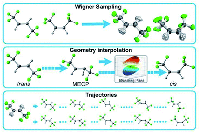 | ||
| Fig. 1 Three initial training set generation approaches in PyRAI2MD. Wigner sampling explores the conformational space near the equilibrium geometries. Geometry interpolation collects the data along with reaction coordinates from reactant to product. Trajectories samples the data from quantum chemical trajectories. The 2D PES data can also supplement the data sampling. Detailed information about the initial training set generation is available in the ESI.† | ||
Our initial training set generation scheme combines Wigner sampling, geometrical interpolation, and trajectories. The Wigner sampling approach generates training data by sampling reactant and product structures. The geometry interpolation approach accesses the reaction coordinate diagram with the optimized reactant, product, and minimum energy crossing point (MECP) geometries. It systematically varies the reactant geometry to that of the minimum energy crossing point and then to that of the product in equal increments of Z-matrix coordinate parameters. We expanded the range of sampled structures in the training data by applying the Wigner sampled geometrical perturbations to the interpolated reaction coordinate diagram. The trajectories approach samples conformations from short-time quantum chemical NAMD trajectories (50–100 fs). For instance, we included every 10th snapshot of the first 50 fs of 132 CASSCF NAMD trajectories of 1 corresponding to the trans → cis isomerization.
2.4 Adaptive sampling
The initial training set represents a chemically intuitive conformational space to fit the NN potential for the investigated photochemical reactions. The NN potential becomes less reliable when trajectories frequently encounter the structures outside the data set. We efficiently expanded the initial training set to cover important structures on the PESs using an active learning approach, adaptive sampling. It was first introduced by Behler et al.36 then adapted to ground- and excited-state dynamics by Marquetand and co-workers.17,37 The adaptive sampling propagates ML-NAMD trajectories to explore the conformational space and sample the uncertain geometries based on the standard deviation between two sets of NNs. The collected geometries are recomputed with quantum chemical calculations and then join the initial training set to improve the NN potentials iteratively. In the cis–trans isomerization of trans-1, the adaptive sampling included 250 ML-NAMD trajectories in 500 fs with a 0.5 fs timestep at 300 K. The adaptive sampling stopped at 28 iterations with 6207 data points (98% of the trajectories completed without finding new geometries). In the 4π-electrocyclic ring-closing of 3, the adaptive sampling ran 250 ML-NAMD trajectories in 1000 fs with a 0.5 fs timestep. We increased the temperature to 1200 K to access high energy non-equilibrium geometries along the reaction coordinates. The temperature was reset to 300 K in the production ML-NAMD simulations. We obtained a final set of 6272 data points after 100 iterations (96% of the trajectories completed normally). Detailed information about the adaptive sampling is available in the ESI.†3. PyRAI2MD
We developed the Python Rapid Artificial Intelligence Ab Initio Molecular Dynamics program (PyRAI2MD) to integrate ML models and the NAMD algorithms. It is an open-source code to enable ML-NAMD simulations for unprecedented molecular complexity and timescales. Fig. 2 illustrates the computational architecture of PyRAI2MD, which requires ML and NAMD kernels.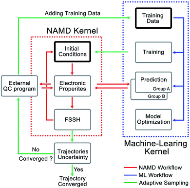 | ||
| Fig. 2 The computational architecture of PyRAI2MD. The bold boxes are the initial stage in NAMD and ML kernel. | ||
The workflow in the NAMD kernel starts with the Wigner sampled initial conditions. The following procedures, red arrows in Fig. 2, iteratively compute the energies, forces, NACs, and surface hopping probability, propagating the NAMD trajectory. We generalized the input and output format of computing energies, forces, and NACs in the NAMD kernel. This feature enables efficient communication between the ML kernel and our chosen external quantum chemical program, OpenMolcas 19.11.21 The workflow in ML kernel reads a training set or an existing model. It provides a convenient interface to train models and make predictions marked by blue arrows in Fig. 2. The green arrows in Fig. 2 illustrate the adaptive sampling workflow incorporating the NAMD and ML kernels. It first loads two trained ML models to run multiple trajectories in the NAMD kernel. The trajectories explore the unsampled conformational space while the two ML models evaluate the prediction uncertainty on-the-fly, as described in Section 2.4 and ESI.† The sampled data were added into the initial set to train a new model.
4. Results and discussion
4.1 Cis–trans isomerization model for trans-hexafluoro-2-butene
As the first demonstration of our ML-NAMD approach, we chose an emblematic photochemical reaction, an isomerization of trans-hexafluoro-2-butene, trans-1. We have characterized the photodynamics of trans-1 with 1371 CASSCF(2,2)/cc-pVDZ trajectories. 946 trajectories correspond to the cis–trans isomerization, whereas 425 trajectories undergo an intramolecular hydrogen abstraction to form hexafluoro-2-butene carbene, 2 shown in Scheme 1.This pathway is consistent with prior theoretical studies on ethylene intramolecular hydrogen migration reactions.38–40 To test whether the NN-driven adaptive sampling method can discover the missing data for the alternative carbene pathway without prior knowledge or human bias, the initial training set only included the information about the trans → cis isomerization of trans-1.
4.2 ML potential for the cis–trans isomerization of trans-hexafluoro-2-butene
We trained four NNs for the cis–trans isomerization of trans-1 with PyRAI2MD. On a single CPU, the predictions of the energies, forces, and NACs take 0.00991 seconds, whereas the equivalent computations at CASSCF(2,2)/cc-pVDZ require 336 seconds. These results represent an NN acceleration of 3.4 × 10⁴-fold relative to ground-truth CASSCF calculations. We summarized the NN architecture, mean absolute error (MAE), and coefficient of determination (R2) of the predicted energies, forces, and NACs in Table 1.| Hyperparameters | Energies, forces | NACsa | ||
|---|---|---|---|---|
| NN1 | NN2 | NN1 | NN2 | |
| a Here the NAC only represents the interstate coupling term. b The MAE and R2 of forces are shown in the parenthesis. | ||||
| Hidden layers | 3 | 5 | 5 | 3 |
| Neurons/layer | 400 | 300 | 300 | 600 |
| Batch size | 64 | 128 | 128 | 128 |
| MAE | 0.023(0.14)b | 0.025(0.15)b | 0.182 | 0.170 |
| R 2 | 0.9989(0.9357)b | 0.9984(0.9536)b | 0.7137 | 0.7423 |
The MAE of predicted energies is 0.023–0.025 that meets the ‘chemical accuracy’ threshold (1 kcal mol−1 = 0.043 eV). The R2 values are 0.9984–0.9989 in NN1 and NN2, suggesting an almost linear correlation between the NN prediction and QC reference. The MAE and R2 in force calculation are 0.14–0.15 eV Å−1 and 0.9357–0.9536. These values are consistent with previous reports on SO2 and CH2NH2+ photochemistry.18 The MAE and R2 in the interstate coupling term of the NACs are 0.170–0.182 eV Å−1 and 0.7137–0.7423, respectively. The low R2 relative to energies and forces suggests possible overfitting of NACs (the training MAE are 0.014–0.015 eV Å−1 and the training R2 are 0.9969–0.9970) due to the indefinite term of the antiderivative of NACs and unavailable training data for it.
4.3 ML-NAMD simulations for the cis–trans isomerization of trans-hexafluoro-2-butene
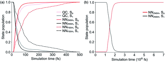
Because the predicted interstate terms of NACs have relatively larger errors than energies and forces, the behavior of NN surface hopping events can be very different from them in QC trajectories. We compared the FSSH and Zhu–Nakamura theory of surface hopping (ZNSH)41–45 to determine the NACs influence on the NN trajectories. The ZNSH method is independent on NACs that has been successfully applied to excited-state dynamics of other systems46,47 and used to train machine learning trajectories.13,14 Propagating a 500 fs NN FSSH trajectory only needs 23 seconds in contrast to 33 hours of running an equivalent trajectory with CASSCF(2,2)/cc-pVDZ. The ZNSH method can further reduce the cost of NN trajectory to 13 seconds because it only computes surface hopping probability near crossing regions (S1/S0 gap < 0.5 eV). We have collected 5573 and 5820 NN trajectories with FSSH and ZNSH methods, respectively. Fig. 3a shows the state population dynamics of trans-1 in 500 fs.The state populations of QC trajectories (Fig. 3a) suggest the S1 half-life is 33.5 fs. The NN FSSH trajectories depending on predicted NACs show rather slower decay of the S1 state. The S1 half-life is 71.0 fs and the MAE in population between the NN FSSH and QC trajectories is 0.105. The NN ZNSH trajectories using NN energies and forces predict that the S1 half-life is 29.0 fs with the MAE in population of 2.5%. The good agreement between the NN ZNSH and QC trajectories indicates the NN energies and forces are sufficiently accurate to detect surface hopping events. The overestimated S1 lifetime in NN FSSH trajectories is attributed to the errors in the NAC model. It seems to underestimate the surface hopping probability, which keeps trajectories at S1 in a longer time until it finds a smaller energy gap for a hop to S0. The S1/S0 gap is similar for QC FSSH and the NNs ZNSH (0.51 eV and 0.46 eV, respectively) while the NN FSSH is 0.12 eV. Due to the closer match, we focused on the ZNSH trajectories in the subsequent discussions.
We tested the limits of our newly established ML-NAMD model by running unprecedented 10 ns simulations with a 0.5 fs time step. We obtained 89 NN ZNSH trajectories and the average state populations are shown in Fig. 3b. The state populations in the first 500 fs also include the 5820 trajectories mentioned above. The non-radiative S1/S0 relaxation completes within 1 ps. The flat population curve after 103 fs indicates all trajectories stayed in S0 up to 10 ns, without surface hopping up to the S1 state. The total 2 × 10⁷ iterations were accomplished in an average of 50 hours on a single CPU. The 10 ns simulation with CASSCF(2,2)/cc-pVDZ would otherwise require approximately 58 years of wall time. We have included the ML-NAMD trajectory video in ESI.†
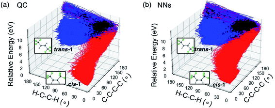
To quantify the difference between the photochemical reaction pathways enumerated by the QC and NN trajectories, we plot the trajectories corresponding to the trans → cis isomerization of trans-1 and their energies with respect to the ∠H–C–C–H and ∠C–C–C–C dihedral angles in Fig. 4.
Fig. 4a illustrates the trace of the QC trajectories that bifurcates toward cis-1 and trans-1. All trajectories started with a narrow spreading in the range of ∠C–C–C–C = 150–180° and ∠H–C–C–H = 0–60° (upper right corner). 248 surface hopping events turned the trajectories along the direction of the ∠H–C–C–H axis toward cis-1. 698 trajectories took the same path returning to trans-1. The trans![[thin space (1/6-em)]](https://www.rsc.org/images/entities/char_2009.gif) :
:![[thin space (1/6-em)]](https://www.rsc.org/images/entities/char_2009.gif) cis ratio is 2.8
cis ratio is 2.8![[thin space (1/6-em)]](https://www.rsc.org/images/entities/char_2009.gif) :
:![[thin space (1/6-em)]](https://www.rsc.org/images/entities/char_2009.gif) 1 in the QC trajectories. The NN predicted trajectories in Fig. 3b recreated the topology of the reference. The NN predicted 772 trajectories transformed to cis-1 and 2680 trajectories back to trans-1, resulting in a corresponding ratio of 3.5
1 in the QC trajectories. The NN predicted trajectories in Fig. 3b recreated the topology of the reference. The NN predicted 772 trajectories transformed to cis-1 and 2680 trajectories back to trans-1, resulting in a corresponding ratio of 3.5![[thin space (1/6-em)]](https://www.rsc.org/images/entities/char_2009.gif) :
:![[thin space (1/6-em)]](https://www.rsc.org/images/entities/char_2009.gif) 1. The NN and QC trajectories show virtually identical evolution of the average ∠C–C–C–C and ∠H–C–C–H angles during the 500 fs simulation (Fig. S14†).
1. The NN and QC trajectories show virtually identical evolution of the average ∠C–C–C–C and ∠H–C–C–H angles during the 500 fs simulation (Fig. S14†).
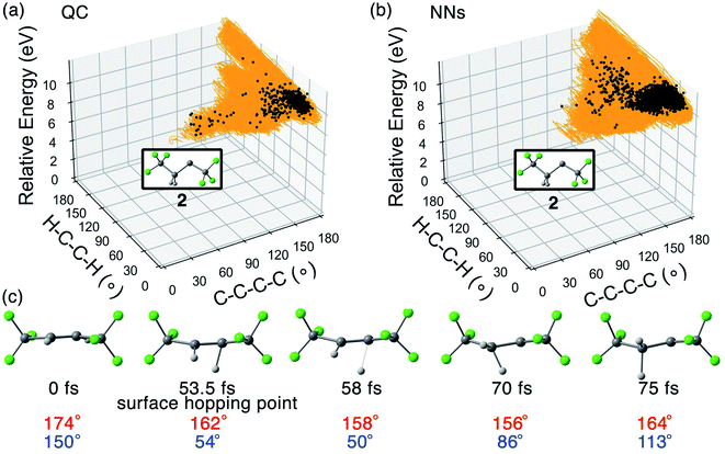
The QC and NN trajectories undergoing the trans → carbene pathway are shown in Fig. 5a and b with 5 snapshots from a QC trajectory in Fig. 5c, including the surface hopping point.
425 QC trajectories formed 2 in a trans![[thin space (1/6-em)]](https://www.rsc.org/images/entities/char_2009.gif) :
:![[thin space (1/6-em)]](https://www.rsc.org/images/entities/char_2009.gif) carbene ratio of 1.6
carbene ratio of 1.6![[thin space (1/6-em)]](https://www.rsc.org/images/entities/char_2009.gif) :
:![[thin space (1/6-em)]](https://www.rsc.org/images/entities/char_2009.gif) 1. The trajectories in Fig. 5a display that the transformation shared the path with trans → cis isomerization from the Franck–Condon region to the S1/S0 crossing region. The S1/S0 surface hopping happened in the area of ∠C–C–C–C = 150–180° and ∠H–C–C–H = 0–60°. In Fig. 5c, the hydrogen migrated to the other carbon atom from 58 to 70 fs. The ∠H–C–C–H angle, 50° at 58 fs, increased to 86° at 70 fs. The C
1. The trajectories in Fig. 5a display that the transformation shared the path with trans → cis isomerization from the Franck–Condon region to the S1/S0 crossing region. The S1/S0 surface hopping happened in the area of ∠C–C–C–C = 150–180° and ∠H–C–C–H = 0–60°. In Fig. 5c, the hydrogen migrated to the other carbon atom from 58 to 70 fs. The ∠H–C–C–H angle, 50° at 58 fs, increased to 86° at 70 fs. The C![[double bond, length as m-dash]](https://www.rsc.org/images/entities/char_e001.gif) C π-bond broke resulting in a nonplanar geometry (∠C–C–C–C = 164° and ∠H–C–C–H = 113° at 75 fs). We intentionally omitted the trans → carbene pathway data in the initial training set, yet the adaptive sampling located 347 structures with significantly broken C–H bonds (>1.40 Å) resembling 2 (5.6% in the final training set). Fig. 5b shows the 2368 NN trajectories toward 2. The predicted trans
C π-bond broke resulting in a nonplanar geometry (∠C–C–C–C = 164° and ∠H–C–C–H = 113° at 75 fs). We intentionally omitted the trans → carbene pathway data in the initial training set, yet the adaptive sampling located 347 structures with significantly broken C–H bonds (>1.40 Å) resembling 2 (5.6% in the final training set). Fig. 5b shows the 2368 NN trajectories toward 2. The predicted trans![[thin space (1/6-em)]](https://www.rsc.org/images/entities/char_2009.gif) :
:![[thin space (1/6-em)]](https://www.rsc.org/images/entities/char_2009.gif) carbene ratio is 1.1
carbene ratio is 1.1![[thin space (1/6-em)]](https://www.rsc.org/images/entities/char_2009.gif) :
:![[thin space (1/6-em)]](https://www.rsc.org/images/entities/char_2009.gif) 1.
1.
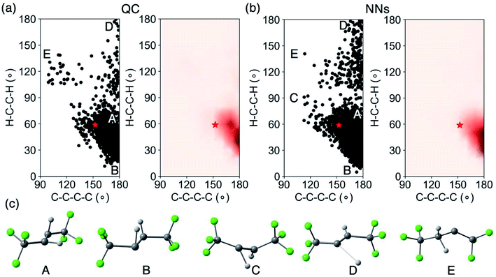
We analyzed the crossing region and surface hopping points for the QC and NN trajectories. Fig. 6 shows the spatial distribution of the latest S1/S0 surface hopping point in each trajectory and examples of surface hopping geometries along the S1/S0 crossing seam.
Fig. 6a projects the latest S1/S0 surface hopping points from the CASSCF(2,2)/cc-pVDZ trajectories into the 2D conformational space of 1. The dense areas represent the S1/S0 crossing region as defined by the two reaction coordinates. In the density map (Fig. 6a, right panel), the surface hopping points accumulated at two regions, ∠C–C–C–C = 170°; ∠H–C–C–H = 60° and ∠C–C–C–C = 180°; ∠H–C–C–H = 40°, which have larger ∠C–C–C–C angels than MECP-trans-1. Beside the hopping points near MECP-trans-1, Fig. 6c shows two pyramidalized surface hopping geometries at A (∠C–C–C–C = 180° and ∠H–C–C–H = 80°) and B (∠C–C–C–C = 180° and ∠H–C–C–H = 20°). We noted C–H stretching surface hopping points at D (∠C–C–C–C = 180° and ∠H–C–C–H = 180°); the C–H distance is 2.24 Å. The surface hopping geometries at E (∠C–C–C–C = 110° and ∠H–C–C–H = 140°) have shown the formation of 2, which suggests that excited-state hydrogen abstraction is theoretically possible. Fig. 6b depicts the distribution and density of NN predicted S1/S0 surface hopping points. These surface hopping events occurred closely at ∠C–C–C–C = 180°; ∠H–C–C–H = 40° agreeing with those observed in QC trajectories. The significant increase in the number of NN trajectories provided an increased statistical significance of our crossing region analysis. The NNs located a twisting surface hopping geometry at C (∠C–C–C–C = 120° and ∠H–C–C–H = 90°). The density map (Fig. 6b, right panel) suggests it is a relatively rare surface hopping event as few points were located at C. The NN could detect the rare event because of the substantially increased number of trajectories (5820) with a nearly negible increase in computational cost.
4.4 4π electrocyclic ring-closing model of norbornyl cyclohexadiene
To demonstrate our ML-NAMD method on a more complex reaction, we studied the photochemical behavior of norbornyl cyclohexadiene 3 (Scheme 2). Burns and Lopez hypothesized that irradiation of 3 would initiate 4π-electrocyclic ring-closing to produce diastereoisomeric ladderene products anti-4 and syn-4, in line with known cyclohexadiene photochemistry.48 Irradiation of 3 with 254 nm light was performed for 0.5, 1, 2, or 4 hours and provided several hydrocarbon products. The anticipated major reaction pathway produced ladderene diastereomers anti-4 (28%) and syn-4 (4%). Under these conditions we also observed an alternative reaction pathway to anti-4′ (8%) via intermediate diene 3′ (see ESI† for more details). We then decided to study the major reaction pathway of 3 to form products anti-4 and syn-4 using our ML-NAMD method.4.5 ML potential for the 4π-electrocyclic ring-closing of norbornyl cyclohexadiene
We trained NNs for 3 as described in Sections 2.3 and 2.4. The NN predict energies, forces, and NACs of 3 with comparable efficiency (0.0118 seconds) to 1 (0.00991 seconds). However, the marked increase in electrons and active space size of 3 results in considerably longer wall time of a single point CASSCF(4,3)/ANO-S-VDZP calculation (2480 seconds) than 1 (336 seconds). Note the ANO-S-VDZP and cc-pVDZ basis sets are the same size. The NN benefit from a 2.1 × 10⁵-fold acceleration compared to the CASSCF calculations. We summarized the NN architecture, MAE, and R2 of predicted energies, forces, and NACs in Table 2.| Hyperparameters | Energies, forces | NACsa | ||
|---|---|---|---|---|
| NN1 | NN2 | NN1 | NN2 | |
| a Here the NAC only represents the interstate coupling term. b The MAE and R2 of forces are shown in the parenthesis. | ||||
| Hidden layers | 3 | 4 | 3 | 4 |
| Neurons/layer | 400 | 300 | 500 | 300 |
| Batch size | 128 | 128 | 128 | 128 |
| MAE | 0.027(0.12)b | 0.031(0.13)b | 0.078 | 0.081 |
| R 2 | 0.9996(0.9934)b | 0.9991(0.9858)b | 0.7956 | 0.5732 |
The MAE of the energy predictions for compound 3 are 0.027–0.031 eV, which approaches chemical accuracy (1 kcal mol−1 or 0.043 eV). The R2 values are 0.9991–0.9996 and demonstrate a good correlation between the predicted and the target energies. The MAE of the forces ranges from 0.12–0.13 eV Å−1, with R2 values ranging from 0.9991–0.9996. They are 0.02 eV Å−1 smaller than in case of compound 1, suggesting improved fitting of forces. The MAE of the S1/S0-coupling are 0.078–0.081 eV Å−1, which are smaller than 50% of that of 1. Nevertheless, possible overfitting of the S1/S0-coupling still occurs as the R2 values (0.5723–0.7956) are relatively low in the validation set (the MAE and R2 are 0.036–0.040 eV and 0.9217–0.9452 in the training set).
4.6 ML-NAMD simulations for the 4π-electrocyclic ring-closing of norbornyl cyclohexadiene
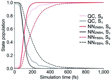
The photodynamics study on 3 requires computationally intensive NAMD simulations. We have obtained 240 CASSCF(4,3)/ANO-S-VDZP trajectories of the 4π-electrocyclic ring-closing of 3. The single trajectory of 1000 fs simulations required an average of 17 days of computation time. With our ML-NAMD method, we propagated 3910 NN FSSH trajectories and 3954 NN ZNSH trajectories, requiring just 56 and 38 seconds, respectively.We compared the QC and NN state populations to assess the errors of our trained NN in predicting excited-state dynamics of 3 (Fig. 7).
Fig. 7 shows that the S1 half-life of the QC trajectories is 108 fs. The NN FSSH trajectories overestimated it to be 175 fs. The resulting MAE in population between NN FSSH and QC trajectories is 14.8% in the first 500 fs. In contrast, the NN ZNSH trajectories agree better with the QC trajectories. The predicted S1 half-is 105 fs and the MAE in population is 4.5%. The delayed surface hopping events in the NN FSSH trajectories resulted from the underestimation of NACs as discussed in Section 4.3. This causes the NN FSSH trajectories to spend longer times on approaching regions with smaller energy gaps. The average surface hopping S1/S0 energy gap is 0.22, which is notably smaller than 0.45 eV in the QC trajectories (0.26 eV in the NN ZNSH trajectories). Thus, the following discussion of the ML-NAMD simulations of 3 will focus on the NN ZNSH trajectories.
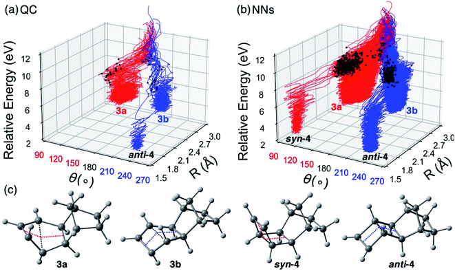
The QC and NN trajectories are characterized with the distance R between the two carbon atoms closing the cyclohexadiene ring and the bending angle θ of the cyclohexadiene plane, shown in Fig. 8a and b. The optimized geometries of observed products and intermediates are shown in Fig. 8c.
The QC and NN trajectories show two types of pathways. We distinguished the syn- and anti-pathways with the bending angle of the cyclohexadiene plane, θ = 120–150° and θ = 210–240°, respectively. 2 of 240 QC trajectories formed anti-4 in 1 ps corresponding to a low yield of 0.8%, while a pathway to syn-4 is absent due to the insufficient number of trajectories. Our calculations suggest that the major outcome of the photoreaction of 3 return to the reactant (Fig. S19†). The higher experimental yield of anti-4 (28%) and syn-4 (4%) is because the reactant can be re-excited to have another chance of ring-closing during the 4 hours of irradiation. Our QC-NAMD simulations also suggest a less direct pathway involving reactive intermediates, 3a and 3b (Fig. 8a and c). The QC trajectories suggest a yield of 3a and 3b are 13% and 7% (Fig. 8a). Among those non-productive trajectories (Fig. S19†), 44% of the trajectories involved syn-configurations, and 35% formed anti-configuration before they reverted to 3. Collectively, from the S1-FC regions, 57% of the trajectories followed the syn-pathway, and 43% of the trajectories pursued the anti-pathway. The preferential syn-pathway in the QC-NAMD simulations agree with the minimum energy path (MEP) calculations of 3 (Fig. S17†) where the syn-pathway is steeper descent than the anti-pathway.
The increase in NN trajectories in Fig. 8b identified a pathway to syn-4, with a 0.2% yield. The yield of anti-4, 3a, and 3b are 0.7%, 11%, and 5%, respectively, resulting in 84% non-productive trajectories reverting to 3. The formations of syn-4 and anti-4 start near 100 fs and complete near 200 fs (Fig. S20†). We compare the yield of syn-4 and anti-4 in the NN trajectories and the experiment by zooming in the 100–200 fs region and normalizing the yield and time scale. The predicted yield curves show excellent agreement with the experiment data (Fig. S21†). Among the non-productive trajectories, 53% preferred the syn-pathway, and 31% went through the anti-pathway (Fig. S19†). Overall, the NN trajectories are consistent with QC trajectories and MEP calculations that the syn-pathway (64%) is preferred over the anti-pathway (36%). It is also worth mentioning that we had not provided any information about the intermediates 3a and 3b in the initial training set since we did not recognize them until running QC-NAMD. The NN effectively collected the necessary training data through adaptive sampling.
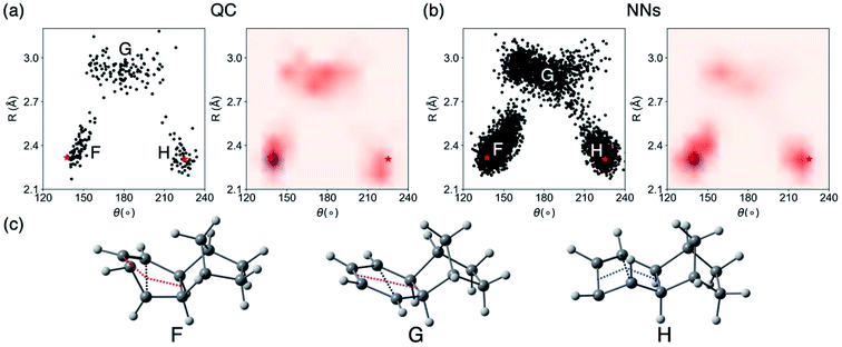
We then analyzed the QC and NN surface hopping geometries to understand the behavior of NN trajectories in the crossing regions. Fig. 9a and b plot the distributions and density of the last S1/S0 surface hopping geometries in the QC and NN trajectories. Fig. 9c illustrates examples of three surface hopping geometries.
The 2D projection of surface hopping geometries from the QC trajectories shows three distinct regions (Fig. 9a). The crossing region around F and H resemble the MECP geometries along the syn- and anti-pathway, MECP-syn-3 and MECP-anti-3 (Fig. S16†). These geometries show shortened C–C distances (R = 2.2–2.6 Å) and bent cyclohexadiene plane (θ = 140–160° near F and θ = 210–230° near H) that are distorted toward the 4π-electrocyclic ring-closing. The region F is denser than H indicating the syn-pathway is preferred. Another crossing region G corresponds to cyclohexadiene-like surface hopping geometries (R = 2.8–3.2 Å, θ = 150–210°). These surface hopping events occur via the stretching of the cyclohexadiene plane. Fig. 9b plots surface hopping geometries in the NN trajectories. The distributions are similar in the three crossing regions. According to the density map, the NN tend to predict more surface hopping at the ring-closing regions (F and H) than the stretching region (G).
In the non-productive trajectories, we observed thermal conversions from 3a and 3b to 3. Fig. 10 depicts the QC trajectories snapshots showing the conversion from 3a to 3 after it hops to the ground-state.
 | ||
| Fig. 10 Snapshots of the formation of transient intermediate 3a in a CASSCF(4,3)/ANO-S-VDZP trajectory. The trajectory first formed 3a at 122.5 fs and then converted to 3 at 331.5 fs. | ||
The snapshot in Fig. 10 shows a first appearance of 3a is at 122.5 fs. It completely transformed to 3 at 331.5 fs suggesting a lifetime of 209 fs. The trajectory statistics concludes that 0.8% of the QC trajectories undergo 3a → 3 conversion and 0.8% go for 3b → 3. The NN trajectories confirm the 3a → 3 and 3b → 3 thermal conversions in 5% and 3% of the trajectories, respectively. The remaining 3a and 3b at the end of the NAMD simulations suggest the lifetime of 3a and 3b can be longer than 1 ps. That encourages us to explore subsequent thermal reactions of the photodynamics of 3 in nanosecond scale.
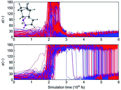
We continued to propagate 984 NN trajectories from 1 ps to 1 ns, which completes in just 4.8 hours per trajectory. We monitored the interconversion from 3a and 3b to 3 with the ∠H–C–C–H dihedral angles a, as shown in Fig. 11.
The top panel in Fig. 11 illustrates trajectories that formed the aforementioned short-lived 3a and 3b, which convert to 3 within 1 ps. The dihedral angle a is below 60° in the initial 100 fs. The formation of 3a and 3b rotate the C![[double bond, length as m-dash]](https://www.rsc.org/images/entities/char_e001.gif) C bond leading to a = 180° and the continued conversion to 3 recovery the planar cyclohexadiene with a < 30°. The bottom panel in Fig. 11 shows the trajectories involved with a long-lived 3a and 3b. The trajectories retain the dihedral angle a = 180° at 1 ps. By tracking reaction coordinate a, we note that the earliest conversion occurred right after 1 ps and the last one appeared at 0.9 ns. In the end of 1 ns simulation, the yield of 3a reduced to 1% and the 3b completely converted to 3. Measuring the ∼0.9 ns lifetime of these reactive intermediates would not be possible without ML-NAMD simulations; this dynamic effect offers important mechanistic insight into photochemical ladderene formation reactions.
C bond leading to a = 180° and the continued conversion to 3 recovery the planar cyclohexadiene with a < 30°. The bottom panel in Fig. 11 shows the trajectories involved with a long-lived 3a and 3b. The trajectories retain the dihedral angle a = 180° at 1 ps. By tracking reaction coordinate a, we note that the earliest conversion occurred right after 1 ps and the last one appeared at 0.9 ns. In the end of 1 ns simulation, the yield of 3a reduced to 1% and the 3b completely converted to 3. Measuring the ∼0.9 ns lifetime of these reactive intermediates would not be possible without ML-NAMD simulations; this dynamic effect offers important mechanistic insight into photochemical ladderene formation reactions.
5. Concluding remarks
We have applied and expanded a ML-NAMD approach using neural networks that overcome current limitations in photodynamics simulations, including simulation time and molecular complexity. We used a composite generation scheme to effectively sample the initial training set, which combines the Wigner sampling, geometrical interpolations, and short-time quantum chemical trajectories. We implemented an adaptive sampling workflow to automatically expand the initial training set with the important data in the unexplored conformational space using a query of committee model. The final data set of the cis–trans isomerization and 4π-electrocyclic ring-closing models has 6207 and 6267 data points, respectively. The training error in energy achieved chemical accuracy with a mean absolute error of 0.023–0.032 eV. The forces and NAC interstate couplings errors were 0.12–0.15 eV Å−1 and 0.078–0.182 eV Å−1 respectively.For the cis–trans isomerization of trans-1, the NNs effectively accelerated the computations of energies, forces, and NACs for trans-1 in 3.4 × 10⁴-fold compared to the CASSCF calculations. The 10 ns ML-NAMD simulations from the S1 Franck–Condon regions of the Wigner sampled initial conditions at 300 K on a single CPU completed in 2 days 2 hours on average of 89 trajectories, which would have approximately required 58 years for running the CASSCF(2,2)/cc-pVDZ calculations. The analysis of 5820 NN trajectories in 500 fs shows consistent results with the QC trajectories, predicting the formation of cis-1 (trans![[thin space (1/6-em)]](https://www.rsc.org/images/entities/char_2009.gif) :
:![[thin space (1/6-em)]](https://www.rsc.org/images/entities/char_2009.gif) cis = 3.5
cis = 3.5![[thin space (1/6-em)]](https://www.rsc.org/images/entities/char_2009.gif) :
:![[thin space (1/6-em)]](https://www.rsc.org/images/entities/char_2009.gif) 1) and 2 (trans
1) and 2 (trans![[thin space (1/6-em)]](https://www.rsc.org/images/entities/char_2009.gif) :
:![[thin space (1/6-em)]](https://www.rsc.org/images/entities/char_2009.gif) carbene = 1.1
carbene = 1.1![[thin space (1/6-em)]](https://www.rsc.org/images/entities/char_2009.gif) :
:![[thin space (1/6-em)]](https://www.rsc.org/images/entities/char_2009.gif) 1). The NN acceleration becomes more significant (2.1 × 10⁵-fold) for complex organic molecules such as 3 because of the considerably increasing cost of CASSCF calculations with more electrons and larger active space. Our results of 3954 NN trajectories in 1 ps confirmed the low-yield of syn-4 (0.2%) and anti-4 (0.7%) that support our experimental results. The continued 1 ns NN photodynamics simulations revealed almost complete thermal conversion from 3a and 3b to 3, which explain their absence in experiment.
1). The NN acceleration becomes more significant (2.1 × 10⁵-fold) for complex organic molecules such as 3 because of the considerably increasing cost of CASSCF calculations with more electrons and larger active space. Our results of 3954 NN trajectories in 1 ps confirmed the low-yield of syn-4 (0.2%) and anti-4 (0.7%) that support our experimental results. The continued 1 ns NN photodynamics simulations revealed almost complete thermal conversion from 3a and 3b to 3, which explain their absence in experiment.
We have demonstrated that the PyRAI2MD ML-NAMD approach is able to not only reproduce experimental results, but can be used to identify new light-induced mechanistic pathways. The identification of reactive intermediates such as the carbene 2 and isomers 3a and 3b help to explain experimental results. Our study provides a path forward to quantify the lifetimes of reactive long-lived excited-states and reactive intermediates currently inaccessible with quantum chemical methods alone. We anticipate that these PyRAI2MD-enabled simulations will enable other researchers to understand photochemical reactivities and selectivities with thousands of nanosecond trajectories, facilitating connections between excited- and ground-state mechanistic pathways.
Author contributions
Jingbai Li developed Python Rapid Artificial Intelligence Ab Initio Molecular Dynamics (PyRAI2MD) codes, perfomed machine learning and quantum chemical calculations, and prepared the initial draft of the manuscript and ESI. Patrick Reiser implemented the TensorFlow/Keras neural networks interface for PyRAI2MD, prepared the machine learning section in the ESI, and helped review and edit the draft. Benjamin R. Boswell performed the photochemistry experiment of norbornyl cyclohexadiene, and helped prepare the experimental section in the draft and ESI. André Eberhard tested Gaussian Process regression model. Noah Z. Burns supervised the photochemistry experiments, and helped review and edit the draft. Pascal Friederich superivsed the implementation of TensorFlow/Keras neural networks interface, advised the discussions in the machine learning data, and helped review and edit the draft. Steven A. Lopez supervised the development of PyRAI2MD, managed the project administration, reviewed and edited the manuscript revisions, and responded to the submission process.Conflicts of interest
There are no conflicts of interest to declare.Acknowledgements
J. L. and S. A. L. acknowledge Biruk Abreha, Fatemah Mukadum, and Marcus Schwarting for helpful discussion on NNs. J. L., B. R. B., N. Z. B., and S. A. L. acknowledge the Office of Naval Research (ONR N00014-12-1-0828) and the National Science Foundation (NSF-1940307) for funding this research. J. L. and S. A. L. appreciate the assistance from the Northeastern Research Computing Team and access to the computing resources of the Discovery cluster. P. F. acknowledges funding from the European Union's Horizon 2020 Research and Innovation program under the Marie Sklodowska-Curie grant agreement no. 795206.References
- M. D. Karkas, J. A. Porco Jr and C. R. Stephenson, Photochemical Approaches to Complex Chemotypes: Applications in Natural Product Synthesis, Chem. Rev., 2016, 116(17), 9683–9747 CrossRef PubMed.
- A. Gonzalez, E. S. Kengmana, M. V. Fonseca and G. G. D. Han, Solid-state photoswitching molecules: structural design for isomerization in condensed phase, Mater. Today Adv., 2020, 6, 1–21 Search PubMed.
- J. M. Cox, B. Mileson, A. Sadagopan and S. A. Lopez, Molecular Recognition and Band Alignment in 3D Covalent Organic Frameworks for Cocrystalline Organic Photovoltaics, J. Phys. Chem. C, 2020, 124(17), 9126–9133 CrossRef.
- J. Calbo, C. E. Weston, A. J. White, H. S. Rzepa, J. Contreras-Garcia and M. J. Fuchter, Tuning Azoheteroarene Photoswitch Performance through Heteroaryl Design, J. Am. Chem. Soc., 2017, 139(3), 1261–1274 CrossRef PubMed.
- A. K. Saydjari, P. Weis and S. Wu, Spanning the Solar Spectrum: Azopolymer Solar Thermal Fuels for Simultaneous UV and Visible Light Storage, Adv. Energy Mater., 2017, 7(3), 1–4 Search PubMed.
- J. Li and S. A. Lopez, Multiconfigurational Calculations and Nonadiabatic Molecular Dynamics Explain Tricyclooctadiene Photochemical Chemoselectivity, J. Phys. Chem. A, 2020, 124(38), 7623–7632 CrossRef PubMed.
- J. M. Cox and S. A. Lopez, Multiconfigurational dynamics explain photochemical reactivity and torquoselectivity towards fluorinated polyacetylenes, J. Mater. Chem. C, 2020, 8(31), 10880–10888 RSC.
- M. Ben-Nun and T. J. Martínez, Nonadiabatic molecular dynamics: validation of the multiple spawning method for a multidimensional problem, J. Chem. Phys., 1998, 108(17), 7244–7257 CrossRef.
- M. Ben-Nun, J. Quenneville and T. J. Martínez, Ab Initio Multiple Spawning: Photochemistry from First Principles Quantum Molecular Dynamics, J. Phys. Chem. A, 2000, 104(22), 5161–5175 CrossRef.
- S. Hammes-Schiffer and J. C. Tully, Proton transfer in solution: molecular dynamics with quantum transitions, J. Chem. Phys., 1994, 101(6), 4657–4667 CrossRef.
- J. C. Tully, Molecular dynamics with electronic transitions, J. Chem. Phys., 1990, 93(2), 1061–1071 CrossRef.
- J. C. Tully and R. K. Preston, Trajectory Surface Hopping Approach to Nonadiabatic Molecular Collisions: The Reaction of H+ with D2, J. Chem. Phys., 1971, 55(2), 562–572 CrossRef.
- D. Hu, Y. Xie, X. Li, L. Li and Z. Lan, Inclusion of Machine Learning Kernel Ridge Regression Potential Energy Surfaces in On-the-Fly Nonadiabatic Molecular Dynamics Simulation, J. Phys. Chem. Lett., 2018, 9(11), 2725–2732 CrossRef PubMed.
- W. K. Chen, X. Y. Liu, W. H. Fang, P. O. Dral and G. Cui, Deep Learning for Nonadiabatic Excited-State Dynamics, J. Phys. Chem. Lett., 2018, 9(23), 6702–6708 CrossRef PubMed.
- P. O. Dral, M. Barbatti and W. Thiel, Nonadiabatic Excited-State Dynamics with Machine Learning, J. Phys. Chem. Lett., 2018, 9(19), 5660–5663 CrossRef PubMed.
- F. Aleotti, L. Soprani, A. Nenov, R. Berardi, A. Arcioni, C. Zannoni and M. Garavelli, Multidimensional Potential Energy Surfaces Resolved at the RASPT2 Level for Accurate Photoinduced Isomerization Dynamics of Azobenzene, J. Chem. Theory Comput., 2019, 15(12), 6813–6823 CrossRef PubMed.
- J. Westermayr, M. Gastegger, M. Menger, S. Mai, L. Gonzalez and P. Marquetand, Machine learning enables long time scale molecular photodynamics simulations, Chem. Sci., 2019, 10(35), 8100–8107 RSC.
- J. Westermayr, M. Gastegger and P. Marquetand, Combining SchNet and SHARC: The SchNarc Machine Learning Approach for Excited-State Dynamics, J. Phys. Chem. Lett., 2020, 11(10), 3828–3834 CrossRef.
- J. K. Ha, K. Kim and S. K. Min, Machine Learning-Assisted Excited State Molecular Dynamics with the State-Interaction State-Averaged Spin-Restricted Ensemble-Referenced Kohn-Sham Approach, J. Chem. Theory Comput., 2021, 17(2), 694–702 CrossRef PubMed.
- Intergovernmental Panel on Climate Change, Anthropogenic and Natural Radiative Forcing, in Climate Change 2013 – The Physical Science Basis: Working Group I Contribution to the Fifth Assessment Report of the Intergovernmental Panel on Climate Change, Cambridge University Press, 2014, pp. 659–740 Search PubMed.
- I. Fdez Galvan, M. Vacher, A. Alavi, C. Angeli, F. Aquilante, J. Autschbach, J. J. Bao, S. I. Bokarev, N. A. Bogdanov, R. K. Carlson, L. F. Chibotaru, J. Creutzberg, N. Dattani, M. G. Delcey, S. S. Dong, A. Dreuw, L. Freitag, L. M. Frutos, L. Gagliardi, F. Gendron, A. Giussani, L. Gonzalez, G. Grell, M. Guo, C. E. Hoyer, M. Johansson, S. Keller, S. Knecht, G. Kovacevic, E. Kallman, G. Li Manni, M. Lundberg, Y. Ma, S. Mai, J. P. Malhado, P. A. Malmqvist, P. Marquetand, S. A. Mewes, J. Norell, M. Olivucci, M. Oppel, Q. M. Phung, K. Pierloot, F. Plasser, M. Reiher, A. M. Sand, I. Schapiro, P. Sharma, C. J. Stein, L. K. Sorensen, D. G. Truhlar, M. Ugandi, L. Ungur, A. Valentini, S. Vancoillie, V. Veryazov, O. Weser, T. A. Wesolowski, P. O. Widmark, S. Wouters, A. Zech, J. P. Zobel and R. Lindh, OpenMolcas: From Source Code to Insight, J. Chem. Theory Comput., 2019, 15(11), 5925–5964 CrossRef PubMed.
- T. H. Dunning, Gaussian basis sets for use in correlated molecular calculations. I. The atoms boron through neon and hydrogen, J. Chem. Phys., 1989, 90(2), 1007–1023 CrossRef.
- G. Granucci and M. Persico, Critical appraisal of the fewest switches algorithm for surface hopping, J. Chem. Phys., 2007, 126(13), 134114 CrossRef PubMed.
- G. J. Martyna, M. E. Tuckerman, D. J. Tobias and M. L. Klein, Explicit reversible integrators for extended systems dynamics, Mol. Phys., 1996, 87(5), 1117–1157 CrossRef.
- J. Kim, H. Tao, J. L. White, V. S. Petrovic, T. J. Martinez and P. H. Bucksbaum, Control of 1,3-cyclohexadiene photoisomerization using light-induced conical intersections, J. Phys. Chem. A, 2012, 116(11), 2758–2763 CrossRef PubMed.
- K. Pierloot, B. Dumez, P.-O. Widmark and B. r. O. Roos, Density matrix averaged atomic natural orbital (ANO) basis sets for correlated molecular wave functions, Theor. Chim. Acta, 1995, 90(2–3), 87–114 CrossRef.
- R. Pou-Amérigo, M. Merchán, I. Nebot-Gil, P.-O. Widmark and B. O. Roos, Density matrix averaged atomic natural orbital (ANO) basis sets for correlated molecular wave functions, Theor. Chim. Acta, 1995, 92(3), 149–181 CrossRef.
- P.-O. Widmark, P.-k. Malmqvist and B. r. O. Roos, Density matrix averaged atomic natural orbital (ANO) basis sets for correlated molecular wave functions, Theor. Chim. Acta, 1990, 77(5), 291–306 CrossRef.
- P.-O. Widmark, B. J. Persson and B. r. O. Roos, Density matrix averaged atomic natural orbital (ANO) basis sets for correlated molecular wave functions, Theor. Chim. Acta, 1991, 79(6), 419–432 CrossRef.
- J. Westermayr, F. A. Faber, A. S. Christensen, O. A. von Lilienfeld and P. Marquetand, Neural networks and kernel ridge regression for excited states dynamics of CH2NH2+: from single-state to multi-state representations and multi-property machine learning models, Mach. Learn.: Sci. Technol., 2020, 1(2), 1–11 Search PubMed.
- Y. Guan, D. H. Zhang, H. Guo and D. R. Yarkony, Representation of coupled adiabatic potential energy surfaces using neural network based quasi-diabatic Hamiltonians: 1,2(2)A' states of LiFH, Phys. Chem. Chem. Phys., 2019, 21(26), 14205–14213 RSC.
- D. P. Kingma and J. Ba, Adam: A Method for Stochastic Optimization, 2017, https://arxiv.org/abs/1412.6980 Search PubMed.
- M. Abadi, A. Agarwal, P. Barham, E. Brevdo, Z. Chen, C. Citro, G. S. Corrado, A. Davis, J. Dean, M. Devin, S. Ghemawat, I. Goodfellow, A. Harp, G. Irving, M. Isard, Y. Jia, R. Jozefowicz, L. Kaiser, M. Kudlur, J. Levenberg, D. Mane, R. Monga, S. Moore, D. Murray, C. Olah, M. Schuster, J. Shlens, B. Steiner, I. Sutskever, K. Talwar, P. Tucker, V. Vanhoucke, V. Vasudevan, F. Viegas, O. Vinyals, P. Warden, M. Wattenberg, M. Wicke, Y. Yu, and X. Zheng, TensorFlow: Large-Scale Machine Learning on Heterogeneous Distributed Systems, software available fromhttps://tensorflow.org, 2016.
- J. Westermayr and P. Marquetand, Machine learning and excited-state molecular dynamics, Mach. Learn.: Sci. Technol., 2020, 1, 043001 CrossRef.
- J. Westermayr and P. Marquetand, Machine Learning for Electronically Excited States of Molecules, Chem. Rev., 2020 DOI:10.1021/acs.chemrev.0c00749.
- J. Behler, Constructing high-dimensional neural network potentials: a tutorial review, Int. J. Quantum Chem., 2015, 115(16), 1032–1050 CrossRef.
- M. Gastegger, J. Behler and P. Marquetand, Machine learning molecular dynamics for the simulation of infrared spectra, Chem. Sci., 2017, 8(10), 6924–6935 RSC.
- M. Ben-Nun and T. J. Martínez, Photodynamics of ethylene: ab initio studies of conical intersections, Chem. Phys., 2000, 259(2–3), 237–248 CrossRef.
- I. Ohmine, Mechanisms of nonadiabatic transitions in photoisomerization processes of conjugated molecules: role of hydrogen migrations, J. Chem. Phys., 1985, 83(5), 2348–2362 CrossRef.
- W. Zhou, A. Mandal and P. Huo, Quasi-Diabatic Scheme for Nonadiabatic On-the-Fly Simulations, J. Phys. Chem. Lett., 2019, 10(22), 7062–7070 CrossRef PubMed.
- C. Zhu and H. Nakamura, Theory of nonadiabatic transition for general two-state curve crossing problems. I. Nonadiabatic tunneling case, J. Chem. Phys., 1994, 101(12), 10630–10647 CrossRef.
- C. Zhu and H. Nakamura, Theory of nonadiabatic transition for general two-state curve crossing problems. II. Landau–Zener case, J. Chem. Phys., 1995, 102(19), 7448–7461 CrossRef.
- T. Ishida, S. Nanbu and H. Nakamura, Clarification of nonadiabatic chemical dynamics by the Zhu-Nakamura theory of nonadiabatic transition: from tri-atomic systems to reactions in solutions, Int. Rev. Phys. Chem., 2017, 36(2), 229–285 Search PubMed.
- P. Oloyede, G. Mil'nikov and H. Nakamura, Generalized trajectory surface hopping method based on the Zhu-Nakamura theory, J. Chem. Phys., 2006, 124(14), 144110 CrossRef PubMed.
- C. Zhu, K. Nobusada and H. Nakamura, New implementation of the trajectory surface hopping method with use of the Zhu–Nakamura theory, J. Chem. Phys., 2001, 115(7), 3031–3044 CrossRef.
- L. Yu, C. Xu, Y. Lei, C. Zhu and Z. Wen, Trajectory-based nonadiabatic molecular dynamics without calculating nonadiabatic coupling in the avoided crossing case: trans<->cis photoisomerization in azobenzene, Phys. Chem. Chem. Phys., 2014, 16(47), 25883–25895 RSC.
- L. Yu, C. Xu and C. Zhu, Probing the pi->pi* photoisomerization mechanism of cis-azobenzene by multi-state ab initio on-the-fly trajectory dynamics simulation, Phys. Chem. Chem. Phys., 2015, 17(27), 17646–17660 RSC.
- W. G. Dauben and M. S. Kellogg, Photochemistry of cis-fused bicyclo[4.n.0]-2,4-dienes. Ground state conformational control, J. Am. Chem. Soc., 2002, 102(13), 4456–4463 CrossRef.
Footnote |
| † Electronic supplementary information (ESI) available: Machine learning model, the initial training set generation, NACs phase corrections, grid search, and adaptive sampling, the computational cost of ML-NAMD, data and code availability, the QC calculations of hexafluoro-2-butene and norbornyl cyclohexadiene systems, the Cartesian coordinates of optimized geometries, and the experimental details for the norbornyl cyclohexadiene system. See DOI: 10.1039/d0sc05610c |
| This journal is © The Royal Society of Chemistry 2021 |


