
 Open Access Article
 This Open Access Article is licensed under a Creative Commons Attribution-Non Commercial 3.0 Unported Licence
Thermodynamics and kinetics of the amyloid-β peptide revealed by Markov state models based on MD data in agreement with experiment†
Arghadwip
Paul‡
ab,
Suman
Samantray‡
 ac,
Marco
Anteghini§
a,
Mohammed
Khaled
a and
Birgit
Strodel
*ad
ac,
Marco
Anteghini§
a,
Mohammed
Khaled
a and
Birgit
Strodel
*ad
aInstitute of Biological Information Processing: Structural Biochemistry (IBI-7), Forschungszentrum Jülich, 52428 Jülich, Germany. E-mail: b.strodel@fz-juelich.de
bGerman Research School for Simulation Sciences, RWTH Aachen University, 52062 Aachen, Germany
cAICES Graduate School, RWTH Aachen University, Schinkelstraße 2, 52062 Aachen, Germany
dInstitute of Theoretical and Computational Chemistry, Heinrich Heine University Düsseldorf, 40225 Düsseldorf, Germany
First published on 15th April 2021
Abstract
The amlyoid-β peptide (Aβ) is closely linked to the development of Alzheimer's disease. Molecular dynamics (MD) simulations have become an indispensable tool for studying the behavior of this peptide at the atomistic level. General key aspects of MD simulations are the force field used for modeling the peptide and its environment, which is important for accurate modeling of the system of interest, and the length of the simulations, which determines whether or not equilibrium is reached. In this study we address these points by analyzing 30-μs MD simulations acquired for Aβ40 using seven different force fields. We assess the convergence of these simulations based on the convergence of various structural properties and of NMR and fluorescence spectroscopic observables. Moreover, we calculate Markov state models for the different MD simulations, which provide an unprecedented view of the thermodynamics and kinetics of the amyloid-β peptide. This further allows us to provide answers for pertinent questions, like: which force fields are suitable for modeling Aβ? (a99SB-UCB and a99SB-ILDN/TIP4P-D); what does Aβ peptide really look like? (mostly extended and disordered) and; how long does it take MD simulations of Aβ to attain equilibrium? (at least 20–30 μs). We believe the analyses presented in this study will provide a useful reference guide for important questions relating to the structure and dynamics of Aβ in particular, and by extension other similar disordered proteins.
1 Introduction
The amyloid-β peptide (Aβ) plays a central role in the development of Alzheimer's disease (AD), a neurodegenerative disease that currently affects about 50 million people worldwide.1 The aggregation of Aβ is closely linked to the onset and development of AD;2 it is thus of paramount importance to unravel the details of this process. In the past two decades a plethora of biochemical and biophysical studies have been conducted that were aimed at exactly that goal.3 Nonetheless, for various reasons many open questions surrounding the aggregation of Aβ remain. The difficulties in characterizing this process lie in the facts that Aβ is a highly flexible peptide belonging to the class of intrinsically disordered proteins (IDPs) and can follow different aggregation pathways, which may be on- or off-pathway toward the end products of the amyloid aggregation route that are amyloid fibrils composed predominantly of β-sheet structure in a characteristic cross-β conformation. Moreover, different amyloid fibril structures exist for Aβ and an even higher level of polymorphism is found for the intermediate aggregation products.4,5 Other complicating aspects are that the aggregation process operates on a huge range of length and time scales and is highly sensitive to external conditions.6 Moreover, the aggregation behavior depends on the particular alloform of Aβ, which exists in different lengths ranging from of 36 to 43 amino acids that are found as the main components of the amyloid plaques populating the brains of people having AD.7 The two major alloforms are those with 40 and 42 residues, denoted as Aβ40 and Aβ42 in the following. The most abundant form is Aβ40, while Aβ42 is more prone to aggregate and therefore more frequently deposited in amyloid plaques.7Among the multitude of physicochemical techniques that are employed for studying Aβ, molecular dynamics (MD) simulations at the atomic level provide the highest spatial and temporal resolution for capturing the structural and dynamical characteristics of this peptide.8 Many of the simulation studies, yet as also many of the experimental investigations of Aβ are focused on its monomeric state since the properties of the monomers of aggregation-prone peptides and proteins are the determinants of their aggregation behavior.9,10 It has been 15 years since the first all-atom MD simulation of full-length Aβ in solution has been performed.11 Since then, hundreds of simulation studies involving Aβ40 or Aβ42 have been published. During the first ∼10 years of these studies, research groups relied on the common protein and water force fields (FFs) as was usual practice for the simulation of folded proteins, which were the more frequent object of simulation studies at that time. However, as time showed, very different results regarding the structural preferences of Aβ were obtained depending on which of the FFs was used. In fact, as far back as 2012 when we had first reported our first simulation study of Aβ in solution we concluded that ‘proper benchmarking of the protein force fields for unfolded and intrinsically disordered proteins’ was needed.12
Over the years, various FF benchmarks for Aβ and IDPs in general have been performed.13–17 Depending on the FFs tested, the simulation technique employed (i.e., standard MD versus enhanced-sampling MD, like replica exchange MD), the length of the simulations, and the experimental data used for validation, different FFs were identified as the most suited ones. For instance, García et al.13,14 found OPLS-AA18,19 with the TIP3P water model20 and AMBER99SB21 with the TIP4P-Ew water model22 to be the best FFs for Aβ42, while our own benchmark, that included AMBER99SB,21 AMBER99SB*-ILDN,23,24 AMBER99SB-ILDN-NMR,25 and CHARMM22*26 combined with TIP4P-Ew22 as well as OPLS-AA/TIP3P,18–20 identified CHARMM22* as the best FF.17 However, more recent benchmarks revealed that the common FFs from the AMBER, GROMOS, OPLS, or CHARMM family in combination with standard three- or four-point water models produce conformational ensembles for IDPs that are too compact and too biased towards folded structures.27,28 This conclusion can be explained with the parametrization strategy underlying the standard FFs, which aimed at producing the correct structure for folded proteins,29 while IDPs do not adopt a well-defined equilibrium structure in solution, instead sampling an ensemble of fully and/or partially disordered structures.
A number of research groups set out to modify the existing FF parameters such that they capture the structural diversity and flexibility of IDPs, producing less folded and more expanded IDP conformations. These force field modifications include strengthening the water–protein London dispersion interactions,28,30 refining the protein backbone parameters to create more expanded structures or reducing the tendency for certain ordered conformations,31 and/or altering the salt-bridge interactions.31 In a recent effort, D. E. Shaw Research used AMBER99SB*-ILDN23,24 combined with TIP4P-D water28 as a starting point and reparametrized torsion parameters and the protein–water van der Waals (vdW) interaction terms with the aim to develop a FF that provides an accurate model for both folded proteins and IDPs.32 The performance of the resulting FF, called a99SB-disp, was tested for a large benchmark set of 21 experimentally well-characterized proteins and peptides, including folded proteins, fast-folding proteins, weakly structured peptides, disordered proteins with some residual secondary structure, and disordered proteins with almost no detectable secondary structure. In addition, they assessed the accuracy of six other FF/water combinations. Two of these combinations belong to the older FFs that were developed for folded proteins, a99SB*-ILDN/TIP3P (‘a’ standing for AMBER)23,24 and C22*/TIP3P (‘C’ for CHARMM)26 and three combinations specifically designed for IDPs: a03ws containing empirically optimized solute–solvent dispersion interactions,30 a99SB-ILDN/TIP4P-D with increased water dispersion interactions,28 and C36m with refined backbone potentials (which by default is used with CHARMM-modified TIP3P).31 The seventh FF in the benchmark is a99SB-UCB, which is based on a99SB/TIP4P-Ew21,22 and includes modified backbone torsion parameters33 and optimized protein–solvent Lennard-Jones (LJ) parameters34 proposed by Head-Gordon and co-workers. For each of the proteins or peptides in their test set and FFs considered, Robustelli et al. performed 30-μs MD simulations and compared the MD-generated ensembles against a number of experimental data mainly derived from nuclear magnetic resonance (NMR) spectroscopy, and, if available, also from small angle X-ray scattering (SAXS) and fluorescence resonance energy transfer (FRET).32 They concluded that, taking all tested proteins and peptides into consideration, a99SB-disp is the best-performing FF. One of the peptides included in their test set is Aβ40. Based on Fig. 2 of ref. 32, a99SB-disp is, together with C22*/TIP3P, the second best choice following C36m for modeling Aβ40. Interestingly, the performance of a99SB-UCB is not shown in this figure. Though for Aβ40 it was concluded that ‘a99SB-UCB produced excellent agreement with experimental NMR measurements’.32
A question that was not addressed by the study of Robustelli et al. is how good the different FFs are able to reproduce the kinetics of the conformational transitions of the different proteins and peptides. From a FRET study of Aβ40 and Aβ42 it was found that both peptides do not exhibit conformational dynamics exceeding 1 μs,35 which also agrees with the findings from fluorescence measurements using the method of Trp–Cys contact quenching.36 Given the simulation length of 30 μs of the MD data generated by D. E. Shaw Research, we use their data (which were kindly provided by them) to assess the kinetics of Aβ40 as sampled by the different FFs. One of our goals is to determine how much MD sampling is needed to reach convergence with standard MD simulations applied to Aβ. To this end, we evaluate the convergence of intrinsic structural quantities as well as of NMR observables calculated from the MD data. Moreover, we generate Markov state models (MSMs), which, in addition to providing convergence checks, also elucidate the kinetically stable states of Aβ and the transitions between them. This analysis reveals that the length of an MD simulation required for obtaining equilibrated results for Aβ depends on the FF used for modeling the peptide, but usually requires at least 20–30 μs or more. Another finding is that only two of the seven FFs under consideration are able to reproduce both the structural and kinetic data available from experiments of Aβ40, which are a99SB-UCB, which performs by far the best, and a99SB-ILDN/TIP4P-D. We thus conclude that it has now become reality to predict the thermodynamics and kinetics of the amyloid-β peptide based on tens of microsecond of MD data using a99SB-UCB as force field.
2 Methodology
MD trajectories
The 30 μ MD trajectories were generated by Robustelli et al.32 and kindly provided by the authors. All MD simulations were initiated from an Aβ40 structure similar to that found in PDB entry 1BA6,37 which was placed in a cubic box with edge length of 6 nm, and run for 30 μs using following FFs: a03ws, a99SB-ILDN/TIP4P-D, a99SB-UCB, a99SB-disp, C22*/TIP3P, and C36m. The simulations were performed at pH 7 (i.e., the His residues were modeled as neutral) with 50 mM NaCl added and a simulation temperature of 300 K. The subsequent analysis was applied to each of the seven trajectories.For convergence checks some additional simulations were performed. For a99SB-disp and C36m the simulations were extended to 35 μs. To this end, we extracted the last snapshot of the corresponding 30 μs MD simulation and used it as starting structure for the additional 5 μs MD simulation. As MD software we employed GROMACS version 2018.3 (ref. 38) in combination with either a99SB-disp32 or C36m.31 The external conditions were chosen as in the original simulation: 300 K, 50 mM NaCl, pH 7. The peptide was placed in a cubic simulation box with an edge length of 6.0 nm – as chosen by Robustelli et al.32 – and solvated with the corresponding water model and NaCl added, making sure to also neutralize the system. Before the production MD run was started, the energy was minimized using the steepest descent algorithm, followed by equilibration, first in the NVT ensemble with position restraints on the non-hydrogen atoms of Aβ40, afterwards in the NpT ensemble without position restraints. The 5 μs production runs followed, which were realized in the NpT ensemble using a velocity rescaling thermostat with canonical sampling39 with a 0.1 ps time constant for coupling and a Parrinello–Rahman barostat40 with a relaxation time of 2 ps. All bonds involving hydrogen atoms were restrained using the LINCS algorithm,41 which enabled a time step of 2 fs for the integration of the equations of motion. The electrostatic and van der Waals interactions were calculated using the particle mesh Ewald method42 in conjunction with periodic boundary conditions and a real-space truncation at 1.2 nm. For a99SB-UCB33,34 we run 6 × 5 μs MD simulations using the snapshots sampled at t = 5, 10,…, 30 μs of the corresponding 30 μs MD simulation. The same MD protocol as just described was employed for these simulations.
Structural analyses
The trajectories were analyzed using a combination of standard Gromacs-2016.4 package tools,43,44 custom written Tcl scripts in VMD,45 and Python scripts using the MDAnalysis46 and MDTraj47 libraries. As the trajectory files from the Desmond MD package48 are in DCD file format, there was a need for conversion into Gromacs-compatible TRR format. After this, protein conformations were clustered using the clustering algorithm of Daura et al.49 as implemented in Gromacs with a root mean square deviation (RMSD) cutoff of 1.0 nm. To assign secondary structure elements to the protein conformations, the STRIDE algorithm50 was employed. Inter-residue contact maps were constructed by calculating the fraction of structures in which the residue pairs were having at least one pair of atoms within 0.4 nm of each other.Construction of Markov state models
The underlying kinetics of the systems are captured by constructing Markov state models (MSMs) from the MD simulation data using the PyEMMA library in Python.51 The first step towards building an MSM is to choose a suitable distance metric, called feature, for defining the conformational space of the molecule. Here, we describe the conformations in terms of the distances between the Cα atoms. This feature was selected based on VAMP-2 scores, where VAMP stands for Variational Approach for Markov Process.52 This score is part of the VAMP scores family, which represents a set of score functions that can be used to find optimal feature mappings and optimal Markovian models of the dynamics from time series data. For choosing a subset of relevant features for our model construction, we considered three different features: Cα distances, minimum distance between residues, and backbone torsion angles. In order to evaluate which feature is the best and to avoid overfitting, a cross-validation was performed, comparing the VAMP-2 scores of each of the three features computed for three subtrajectories of 10 μs length per force field. From this analysis, the Cα distances emerged as the most suitable feature (Fig. S1 in the ESI†).Next, we reduced the dimension of the space from 703 interatomic distances to 2 collective coordinates by applying time-lagged independent component analysis (TICA), a dimensionality reduction technique that identifies the slowest modes in the feature space by maximizing the autocorrelation of the reduced coordinates,53 and hence is preferred for MSM construction over the more commonly used principal component analysis (PCA), which does not take into account any kinetic information. A density based clustering technique, HDBSCAN54 is then applied to decompose the reduced conformation space into a set of disjoint discrete states and define the trajectory as a sequence of transitions between these states. An MSM can next be built from this discrete trajectory by counting the transitions between the states at a specified lag time (chosen as 100 ns in this work), constructing a matrix of the transition counts and normalizing it by the total number of transitions emanating from each state to obtain the transition probability matrix. In the case of a03ws, the resulting MSM is further coarse-grained into a hidden Markov model (HMM) using the robust Perron cluster analysis (PCCA+),55 which is a fuzzy version of the spectral algorithm for partitioning graphs that assigns each microstate a probability of belonging to a metastable macrostate.56 For the other FFs this coarse-graining step was not required as the MSMs and HMMs turned out to be identical. Finally, whether the final models satisfy the Markovian assumption is verified with a Chapman–Kolmogorov test.57
Calculation of experimental observables
The NMR chemical shifts of the protein backbone atoms were calculated using SPARTA+.58 Dihedral angles (ϕ, ψ) were calculated for each Aβ residue from the MD trajectories and converted into residue-specific backbone scalar 3JHNHα coupling constants using the Karplus equation59 with the coefficient values A = 7.97 Hz, B = −1.26 Hz, and C = 0.63 Hz from Vögeli et al.60 The simulated and experimentally derived coupling constants were compared by calculating χ2 using eqn (1), including the error term Δ = 0.42 Hz:30,35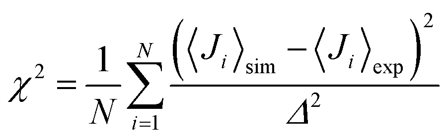 | (1) |
Time-series of the end-to-end distance Ree were calculated as the distance between the Cα atoms of the N- and C-termini of Aβ40 using the MDTraj library47 in Python. From this, the FRET efficiency is calculated as
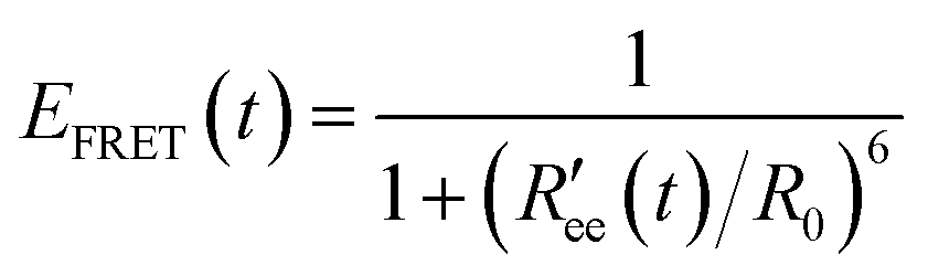 | (2) |
 is calculated by scaling up Ree to account for the effects of the experimental dyes by treating them as 12 extra amino acid residues and assuming a Gaussian scaling exponent,35
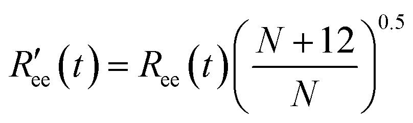 | (3) |
Bayesian reweighting of trajectories by using experimental data
The Bayesian/maximum entropy (BME) technique62 was used to reweight the trajectories and obtain a refined conformational ensemble consistent with selected experimental data, thereby compensating for the discrepancies between the experimental and calculated observables which arise from inaccuracies in the force fields. Here, we considered the J-coupling data to obtain the optimized set of weights for the a99SB-UCB and C36m trajectories.3 Results
We used the 30-μs MD data of Aβ40 from Robustelli et al.32 to (i) assess the convergence of these trajectories, (ii) determine the agreement of the simulated Aβ40 ensembles with spectroscopic data, and (iii) derive the thermodynamics and kinetics of this peptide. The convergence was tested for various structural properties that are usually calculated from MD trajectories, including the structural RMSD, clustering analysis, radius of gyration (Rgyr), and the secondary structure (Section 3.1). Another kind of convergence check is provided by Markov state models (Section 3.2), which is based on kinetically clustering the MD data. Section 3.3 contains the calculation of NMR spectroscopic and FRET observables which allows us to compare the MD generated structural ensembles with experimental findings and to also assess the convergence of these spectroscopic quantities. In Section 3.4 we evaluate the kinetics of Aβ40 and compare the MD results to experimental observations. The structural ensemble of Aβ40 in agreement with the thermodynamic and kinetic data derived from experiments is examined in the Discussion following thereafter.3.1 Convergence checks based on structural data
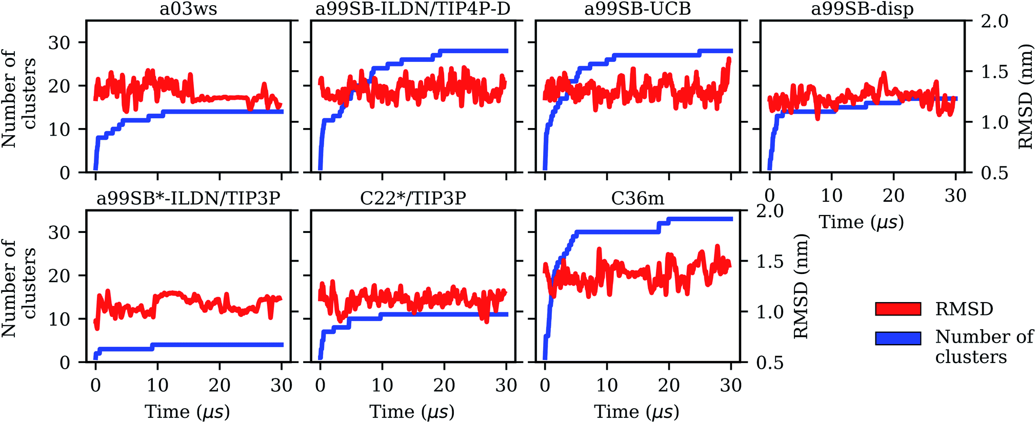 | ||
| Fig. 1 Evolution of the Cα-RMSD with respect to the Aβ40 starting structure of the MD simulations (red, right y-axis) and the number of conformational clusters (blue, left y-axis) for the different force fields (labels on the top of the panels). | ||
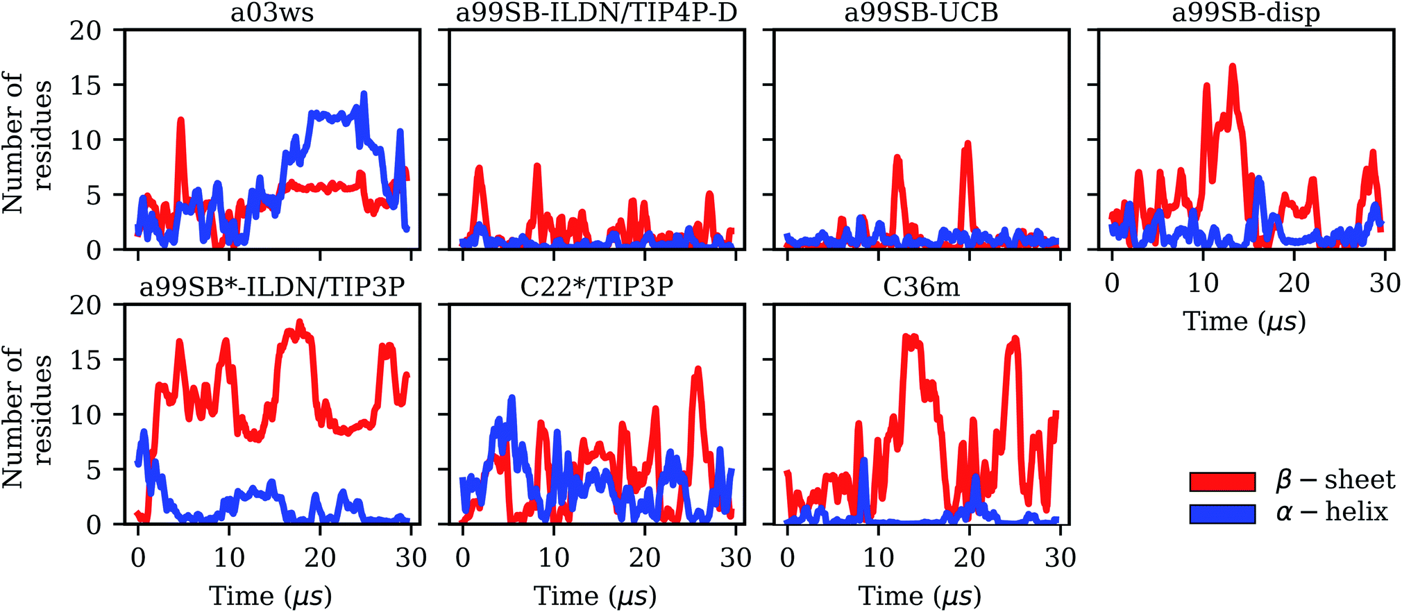 | ||
| Fig. 2 Evolution of the secondary structures β-sheet (red) and α-helix (blue) in terms of the number of Aβ40 residues adopting these structures for the different force fields (labels on the top of the panels). | ||
It is interesting to not only assess time averages for the secondary structure but also its evolution. Fig. 2 reveals that within 10 μs – the time window chosen for averaging – considerable changes in secondary structure can occur. This applies to all FFs yet to different extents. The smallest changes occur for a99SB-ILDN/TIP4P-D and a99SB-UCB, i.e., the two FFs which generally predict a low tendency for Aβ40 to adopt a helical or a β-sheet conformation. Nonetheless, also for these two FFs rare β-sheet formation is observed, requiring simulation times above 10 μs, e.g., at ∼12 and 20 μs in the case of a99SB-UCB. Another extreme is C36m for which huge changes in the amount of β-sheet are observed after 10 μs. It is also interesting to correlate the secondary structure changes to the number of clusters, revealing that even within the same cluster considerable secondary structure changes can occur. This is best seen for the C36m simulation at ∼5–20 μs. During this period, the number of clusters is constant, while the amount of β-sheet formed within Aβ40 first varies widely between 0 and 20%, then increases to more than 40% between 13 and 14 μs, followed by a decrease until no more β-sheet is present at around 18 μs. Thus, the sole analysis of time-averaged secondary structures would have been misleading and should always be augmented by further structural analysis in the case of an IDP as flexible as Aβ.
3.2 Convergence checks based on Markov state models
 | ||
| Fig. 3 Sample densities for different time windows of the trajectories (0–10 μs: yellow, 10–20 μs: cyan, 20–30 μs: magenta) projected along the first two TICA coordinates (TICs) for the different force fields (labels on the top of the panels). It should be noted that the TICs are different between the force fields. | ||
Taking C36m as an example for a detailed analysis of the sample density, one finds that within the first 10 μs Aβ40 largely remained within the same region of the TIC space. Between 10 and 20 μs it explored new conformations (along TIC 1), which, as revealed by the analysis of the secondary structure, resulted from first a build-up of a β-sheet conformation, followed by its destruction. It should be emphasized that TICA identifies the slowest modes in the feature space and not, unlike PCA, the modes of largest motions. TICA thus confirms the result from Fig. 2 that the formation and also disassembly of β-sheets is a slow process in Aβ40, requiring several μs of MD sampling (not only with C36m, but also with.e.g., a99SB-UCB and a99SB-disp). Fig. 3 further shows that after 20 μs of MD with C36m a novel conformational transition, evolving along TIC 2, is explored. Comparison with Fig. 2 reveals that this process again involves β-sheet formation, followed by its disassembly. In the additional 5-μs trajectory, Aβ40 remained in the energy well corresponding to this β-sheet structure (Fig. S4†).
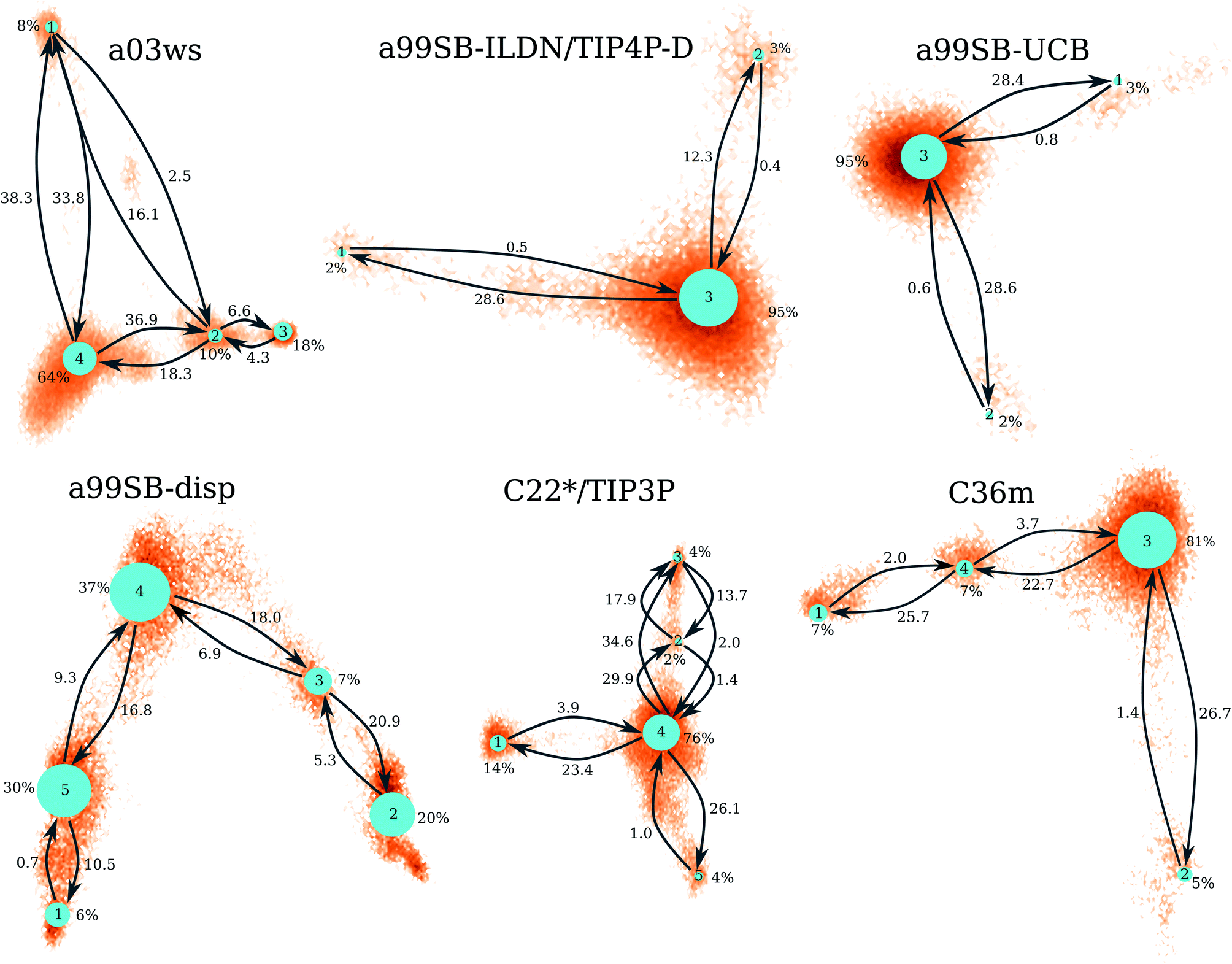 | ||
| Fig. 4 Markov state models for the different force fields (labels above the networks). The size of the network nodes reflects the population of the underlying state (given in % next to the nodes), whereas the transition probabilities are correlated to the mean first passage times (in μs) that are written next to the arrows. The orientation of the MSMs corresponds to the projection of the MD data along the first two TICs in Fig. 3. | ||
The MSM for C36m also involves a dominant state corresponding to a stretched structure with no noteworthy contacts between distant residues (state 3, 81% population). However, with C36m also more compact structures with β-sheets are adopted, yielding MSM states 1, 2 and 4 (19% population in total). These three states exhibit a similar antiparallel β-sheet (Fig. S10†). In states 1 and 4 this involves a β-hairpin centered at residues G25/S26. The β-sheet in state 4 is on-pathway to that of state 1 (coming from state 3) but is shorter than the fully-formed β-sheet of state 4. The latter involves up to 8 or 9 residues per strand and thus reaches up to residue 15 towards the N-terminus and residue 35 towards the C-terminus. This corresponds to the maximum count of 16 to 17 residues that adopt a β-sheet conformation between 13 and 14 μs of the MD simulation (Fig. 2). Another characteristic of the β-sheet in states 1 and 4 is the salt bridge present between D23 an K28, giving rise to the strongest inter-residue contact in either state. While the β-sheet characteristic of state 2 is similar to that of states 1 and 4, it misses the D23–K28 salt bridge, leading a less pronounced turn around G25/S26 and weaker contacts in the adjacent residues.
Similar β-sheet formation is observed with C22*/TIP3P and a99SB-disp, yet the β-sheets are less pronounced (a99SB-disp, Fig. S8†) and may also occur in the N-terminal half of the peptide (C22*/TIP3P, Fig. S9†). Furthermore, the MSMs for these two FFs do not feature a state representing an elongated Aβ40 structure. Instead, more structure formation is seen which also involves helical elements seen in the C-terminal half of the peptide in states 2 and 3 of the MSM obtained with C22*/TIP3P. These two states, however, are only characterized by a low population (2 and 4%, respectively), while the most populated state observed with this FF is associated with a low interpeptide contacts probability (state 4, 76% population) close to an elongated structure. The four states of the MSM for a03ws all feature a β-sheet in the first 10 N-terminal residues, but differ from each other in their contacts in the rest of the peptide (Fig. S5†). Helices of various lengths and locations along the sequence are present in states 1–3, while the most populated state 4 (64% population) is without noteworthy inter-residue contacts beyond residue 10, thus representing a mainly elongated structure.
Comparison between Fig. 3 and 4 (the MSMs from Fig. 4 can be superimposed onto the sample density in Fig. 3 as the same TIC space is used for their projection) show that several of the metastable MSM states were only sampled in the last 10 μs. This holds, for instance, true for state 1 of the MSM with a03ws and also state 2 of the MSM with C36m. The calculation of the mean first passage times (MFPTs) for the transitions between the metastable states confirms that the slowest transitions require more than 20 μs for them to occur. In some cases the MFPTs are even predicted to be larger than 30 μs. Such slow transitions are found in all of the MSMs shown in Fig. 4. As this work aims to provide an answer to the question how much MD sampling is needed before the equilibrium distribution of Aβ is reached, based on the MFPTs the answer would be that at least 30 μs are required.
3.3 Validation of simulated Aβ40 ensembles based on spectroscopic data
In order to validate the simulation results, we compare the structural ensembles obtained for Aβ40 with the corresponding information deduced from spectroscopic data, which is NMR chemical shifts and J-couplings63 as well as FRET efficiencies.35 The FRET experiments were performed at almost identical external conditions as the simulations, which are 297 K as temperature and 50 mM ionic strength in the FRET experiments as opposed to 300 K and also 50 mM ionic strength in the simulations. The NMR experiments, on the other hand, were conducted at 277 K and an ionic strength of 20 mM. Such changes in external conditions are expected to slightly affect the conformational ensemble of Aβ40. A perfect agreement between the results derived from NMR spectroscopy and simulations can thus not be expected.| Quantity | Force fields | ||||||
|---|---|---|---|---|---|---|---|
| a03ws | a99SB-ILDN/TIP4P-D | a99SB-UCB | a99SB-disp | a99SB*-ILDN/TIP3P | C22*/TIP3P | C36m | |
| a For the calculation of the RMSD with respect to the RC chemical shifts, the RC values and correction factors determined in ref. 65 and 66 for IDPs at 300 K and pH 7 were used. b S.D. = standard deviation. | |||||||
| RMSDexp Cα-shift (ppm) | 0.738 | 0.589 | 0.641 | 0.631 | 0.759 | 0.688 | 0.634 |
| RMSDRC Cα-shift (ppm)a | 0.678 | 0.555 | 0.593 | 0.580 | 0.706 | 0.627 | 0.572 |
| RMSDexp C′-shift (ppm) | 1.025 | 0.964 | 0.927 | 0.929 | 0.984 | 0.961 | 0.978 |
| RMSDRC C′-shift (ppm)a | 1.211 | 1.077 | 1.041 | 1.117 | 1.209 | 1.188 | 1.177 |
| χ 2 J-coupling | 7.03 | 3.28 | 1.94 | 4.50 | 6.33 | 2.50 | 3.05 |
| 〈Ree〉 ± S.D. (nm)b | 2.64 ± 1.60 | 3.97 ± 1.53 | 4.22 ± 1.68 | 3.17 ± 1.25 | 2.22 ± 0.82 | 2.67 ± 1.14 | 3.09 ± 1.54 |
| 〈EFRET〉 ± S.D. | 0.83 ± 0.26 | 0.65 ± 0.31 | 0.59 ± 0.33 | 0.81 ± 0.23 | 0.96 ± 0.06 | 0.88 ± 0.17 | 0.80 ± 0.27 |
| 〈Rgyr〉 ± S.D. (nm) | 1.31 ± 0.30 | 1.65 ± 0.30 | 1.76 ± 0.40 | 1.38 ± 0.30 | 1.11 ± 0.08 | 1.24 ± 0.20 | 1.45 ± 0.30 |
| 〈Rhyd〉 ± S.D. (nm) | 1.62 ± 0.16 | 1.77 ± 0.13 | 1.80 ± 0.13 | 1.66 ± 0.11 | 1.53 ± 0.05 | 1.60 ± 0.11 | 1.69 ± 0.13 |
Bax and co-workers concluded from their NMR studies that both Aβ40 and Aβ42 predominantly sample random coil (RC) structures.63 To better estimate how much the simulated ensembles deviate from random coil, we calculated the RMSDs between the simulated and RC chemical shifts using a data set derived for chemical shifts of IDPs,65,66 which was also employed in ref. 63 (Table 1). The RMSD rankings with respect to the experimental chemical shifts and with respect to the RC values are almost identical. In both cases the largest deviations are found for a03ws and a99SB*-ILDN/TIP3P. Closest to RC structures are the structural ensembles generated with a99SB-ILDN/TIP4P-D, a99SB-UCB and a99SB-disp. These findings agree with our conclusions drawn from the MSMs in conjunction with an inter-residue contact analysis for the resulting states. Interestingly, C36m, which was purposefully developed for IDPs,31 leads to less RC in the structures of Aβ40, which was also observed in the contact maps of the MSM states as three of the four MSM states feature rather high β-sheet formation (Fig. S10†). The analysis of the deviations of the simulated chemical shifts from the experimental and RC ones (yielding the secondary chemical shifts) on a per-residue basis reveals a very similar pattern (Fig. S12†). In both cases and for all FFs the largest deviations are found for V24, K28, I32 and V36. For these residues, the measured and RC C′-chemical shifts are considerably larger than the calculated ones. Comparison of the measured and RC C′-chemical shifts revealed deviations opposite in sign (but smaller in absolute terms) for these four residues (Fig. 1 in ref. 63). The experimental values suggest that these residues have a tendency to adopt a helical conformation. Under consideration of all of the up to 12 measured NMR parameters this tendency was confirmed for V24 and K28 by the MERA program (Maximum Entropy Ramachandran map Analysis from NMR data)67,68 that was developed by the Bax lab and applied to the Aβ40/42 NMR data.63 For I32 the measured secondary chemical shift is small, while for V36 a preference for RC is found if all other NMR data measured for that residue are considered. For the region A30–I32 all the predicted C′-chemical shifts are smaller than the experimental values for all FFs. The smallest deviation is found with a99SB-UCB, which also explains the overall smaller RMSD from experiment found for this FF. Comparison with the RC values shows that with a99SB-UCB this region is in a RC state, which is in line with the experimental findings, while the other FFs sample to some degree a β-conformation here.
Another region that needs attention is V17–A21 forming the central hydrophobic core (CHC), which by many studies is proposed to adopt a β-conformation and play a central role during amyloid aggregation of Aβ.8 There is almost no deviation between simulation and experiment for V18 and F19, while for the other residues and also the neighboring K16 and E22 the simulations (apart from the one with a03ws) lead to smaller C′-chemical shifts than in experiment. The predicted values are also smaller than the RC chemical shifts, indicating that this region tends to adopt a β-conformation in the simulations, which was also seen in several of the MSM states for most of the FFs. The NMR data, on the other hand, indicate β-strand formation only for V18–F20, which follows from the measured secondary chemical shifts and also from the MERA analysis that considers the other NMR data.63 However, Bax and co-workers excluded β-sheet formation for that region as from their NMR data no matching set of residues with which to pair these residues in a β-sheet could be identified. In the simulations these residues usually pair with I30–L34 (Fig. S5–S10†), which, as already discussed above, also tend to be in a β-conformation.
For the remaining four FFs the assessment is somewhat more complicated. The usage of a99SB-ILDN/TIP4P-D can be recommended as χ2 for the 3JHNHα couplings is also still considerably small with a value of 3.28; though a99SB-UCB performs clearly better. Interestingly, a99SB-disp, which was developed for IDPs (but also folded proteins) and claimed to be one of the best FFs for Aβ40,32 does not yield 3JHNHα couplings in agreement with experiment. The χ2 value is 4.50 and comparison of the J-couplings on a per residue basis (Fig. 5) shows that for most residues these values are smaller than the experimental J-couplings, only reaching values of ∼6 Hz or less. An exemption to this is the region K16–E22 where the CHC residues V18–F20 in particular demonstrate a tendency to adopt β-conformation, which is also correctly reflected by the J-couplings. Here, a very good agreement with the experimental values is obtained for a99SB-disp. For the other residues, on the other hand, the average ϕ values must be too small. To validate this conclusion we analyzed the Ramachandran angles of I31 and I32 as sampled in the MD simulations in detail (Fig. S13†). From experiment, 3JHNHα couplings above 7 Hz were obtained, indicating a considerable population of extended structures, which is supported by MERA.63 Fig. S13† shows that with a99SB-disp only few structures with ϕ < −90° were sampled for I31 and I32. Instead, polyproline II (PPII) conformations were preferentially adopted, which explain the low J-couplings. With a99SB-ILDN/TIP4P-D and a99SB-UCB, on the other hand, which both led to a good agreement for the J-couplings of I31 and I32, a considerable amount of conformations with ϕ < −120° were sampled, which includes extended conformations from the β-basin as well from the type I β-turn region. Interestingly, with these two force fields the largest variability of conformations was adopted. Basically all allowed regions of the Ramachandran space, including the αL region were sampled, which agrees with the notion that random coil is not a particular structure but a fast fluctuation between all possible ϕ/ψ combinations.
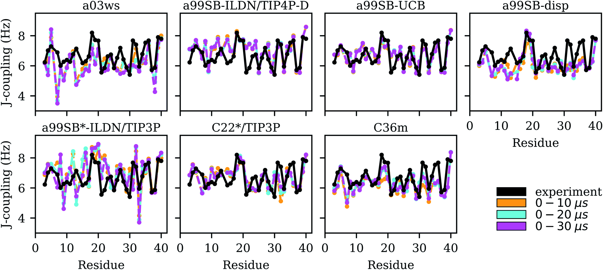 | ||
| Fig. 5 Experimental (black) and simulated (0–10 μs: yellow, 0–20 μs: cyan, 0–30 μs: magenta) 3JHNHα couplings for each Aβ40 residue for the different force fields (labels on the top of the panels). | ||
For the two Charmm FFs under consideration, the situation is contrary to that of a99SB-disp. For C22*/TIP3P and C36m the agreement with NMR chemical shifts is largely insufficient, while the χ2 values for the 3JHNHα couplings are satisfactory (2.50 and 3.05, respectively). Interestingly, the FF not improved for IDPs, i.e., C22*/TIP3P performs somewhat better for both chemical shifts and J-couplings compared to C36m. However, the disagreement between both FFs is limited to a few residues, such as D7, M35 and V36 where C36m performs worse for the J-couplings, while for most of the remaining residues similar NMR observables are predicted. For M35 and V36, C36m sampled a high amount of PPII and αR structures, for M35 also αL (based on the corresponding Ramachandran plots, not shown), leading to J-couplings below those found from experiment, which however, as Fig. 5 shows, increased for sampling times above 10 μs. In general, we observed that it was only beyond 10 μs simulation times that MD convergence for the J-couplings was obtained. This conclusion excludes a99SB-ILDN/TIP4P-D and a99SB-UCB, for which converged J-couplings were already obtained within 10 μs.
 here. To account for the size of the fluorophores, eqn (3) is applied, yielding an average end-to-end distance of ∼4.3 nm for Aβ40. The values for Ree and the FRET efficiencies in Table 1 show that a99SB-UCB performs very well and a99SB-ILDN/TIP4P-D does well in reproducing these observables. While a99SB-disp and C36m are next in performance, they however clearly underestimate Ree, leading to overestimated FRET efficiencies of 0.81 and 0.80, respectively. Even more compact Aβ40 structures are produced by C22*/TIP3P and a99SB*-ILDN/TIP3, with the latter FF leading to average FRET efficiencies of nearly 1 (EFRET = 0.96). For a03ws the situation is somewhat more complicated. The distributions of Ree averaged over different times (Fig. 6) shows that for most FFs this quantity converged within 10 μs. Exceptions are a03ws and a99SB*-ILDN/TIP3P. With the former FF, the end-to-end distance became smaller with time, with a pronounced peak that developed at Ree ∼1.2 nm. With a99SB*-ILDN/TIP3P, on the other hand, the peak at Ree ∼0.9 nm became less important with time, while more extended structures were adopted. The evolution of Ree over the whole trajectory (Fig. S14†) reveals that with a03ws large fluctuations with respect to the end-to-end distance occurred, involving the formation of a compact conformation with especially low Ree values in which Aβ40 was trapped between 16 and 25 μs. Representative conformations from this trapped state are shown in Fig. S15.† They are characterized by the presence of helices along the sequence from residue Y10 onward, corresponding to MSM states 1, 2 or 3. This finding is surprising as the increase in van der Waals interactions between protein and water as done in the development of a03ws was thought to avoid such overly compact protein states,30 yet the current 30 μs MD simulation shows that the helical propensity present in the FF predecessor a03 (ref. 69) overrules this modification if simulated long enough. With the other FFs such trapping is not seen; instead, fast fluctuations in Ree are sampled, with C36m showing the largest and C22*/TIP3P and a99SB*-ILDN/TIP3 the smallest fluctuations.
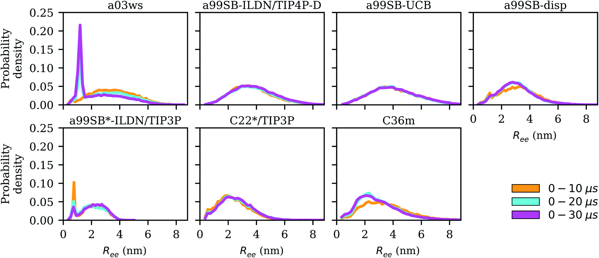 | ||
| Fig. 6 Distribution of the end-to-end distance Ree for increasing trajectory lengths (0–10 μs: yellow, 0–20 μs: cyan, 0–30 μs: magenta) for the different force fields (labels on the top of the panels). | ||
While the agreement between average FRET efficiencies determined experimentally and those derived from the simulations with a99SB-ILDN/TIP4P-D and a99SB-UCB is very good, the same cannot be said for the distribution of the FRET efficiencies. In experiments this distribution assumes a Gaussian shape around the average value,35 while we find highly skewed distributions with the maximum for FRET efficiencies being close to one (Fig. S16†). The same observation was made in other simulation studies where, as observed here with a99SB-ILDN/TIP4P-D and a99SB-UCB, the agreement with the average EFRET value was associated with a considerable amount of structures with Ree values above 6 nm.35,61,70 Further simulations are needed to identify the source of this disagreement. There, effects of the FRET labels including the extra amino acids added at the termini of Aβ should be explicitly considered as well as the orientation of donor and acceptor with respect to each other be accounted for when determining EFRET. Another possible source for the discrepancies between simulations and experiment could lie in the size of the cubic simulation boxes with an edge length of 6 nm used in the simulations analyzed here and in those generated by Head-Gordon et al.,61 while Best and co-workers set up an even smaller box with only 5.5 nm edge length.35 Comparison with Ree shows that Aβ40 can reach beyond these box dimensions if fully extended, which may limit further expansion of the peptide. Thus, in future simulations of Aβ larger boxes should be employed. However, the current results are not expected to be much influenced by the box sizes as in recent coarse-grained simulations of Aβ with implicit solvent, which do not involve simulation boxes, very similar EFRET distributions as in the explicit-solvent all-atom simulations were obtained.70
Another quantity closely related to Ree is the hydrodynamic radius, Rhyd, which was determined as 1.6 nm for Aβ40 at 298 K using size exclusion chromatography (SEC) and NMR diffusion experiments.71 In general, the hydrodynamic radius is closely related to the radius of gyration. For IDPs, a relationship between these two quantities was derived that explicitly takes the chain-length dependency into account.72 Using eqn (7) of ref. 72, we calculated the average Rhyd value for each FF using the Rgyr values determined for the corresponding MD snapshots. The results in Table 1 show that the experimental Rhyd value of 1.6 nm is best reproduced by a03ws and C22*/TIP3P, followed by a99SB-disp and C36m. With a99SB*-ILDN/TIP3P the hydrodynamic radius is underestimated, while a99SB-ILDN/TIP4P-D and a99SB-UCB lead to Rhyd values clearly above the experimental prediction. These observations are mostly in contrast to the conclusions drawn from the calculation of EFRET since for Ree the best agreement was identified for a99SB-ILDN/TIP4P-D and a99SB-UCB. Only for a99SB*-ILDN/TIP3P both Ree and Rhyd agree with each other, both being too small compared to experiment as a result of too compact Aβ40 structures being sampled with this FF. Since for all other quantities a99SB-ILDN/TIP4P-D and a99SB-UCB produced the best agreement with experiment, we decided to disregard the assessment based on Rhyd, especially since it contradicts the Ree results.
3.4 Validation of simulated Aβ40 kinetics based on spectroscopic data
The kinetic analysis of the MD data using MSMs allows to further assess the accuracy of the simulation data based on time scales that were reported for Aβ motions. From the FRET study mentioned above35 it was concluded that Aβ40 and Aβ42 exhibit no conformational dynamics exceeding 1 μs and that the end-to-end distance relaxation time is ∼35 ns, which was determined by nanosecond fluorescence correlation spectroscopy. The upper limit of 1 μs for internal motions agrees with the findings from fluorescence measurements using the method of Trp–Cys contact quenching, which revealed a time scale of ∼1 μs for intramolecular reorientation or diffusion for Aβ40.36 With NMR spin relaxation measurements the faster motions of Aβ40 were studied, from which a timescale of ∼5 ns was determined for segmental motions, which can reach up to ∼10 ns for selected residues.73 The focus of MSMs is the identification of slow, memoryless motions. Thus, for the current comparison of the Aβ40 kinetics as determined by experiment and MD simulations, the upper limit of 1 μs for the slowest motion is of interest to us. All FFs with conformational transitions exceeding this time scale can be rendered as inadequate for modeling the kinetics of Aβ. Here it should be emphasized that the MFPTs discussed above refer to well-defined transitions between specified states, which are not the same as the relaxation times probed by the different spectroscopic techniques. For this, the implied time scales (ITSs) underlying the constructed MSMs are better suited. The implied time scales reflect how quickly any initial state vector converges towards the equilibrium state vector in an MSM and are thus comparable to relaxation times monitored experimentally. The MFPTs, on the other hand, indicate the time it takes to transition from one equilibrium state vector to another one. This can become considerably larger than the ITSs, especially for transitions into equilibrium states with very small probabilities, which can be seen from the MFPTs in Fig. 4. Thus, we concentrate on the ITSs here.The plots of the ITSs against the lag times of the MSMs (Fig. S17†) show that in the case of a03ws, a99SB-disp, C22*/TIP3P and C36m they clearly exceed 1 μs. Some of these FFs even reach time scales for the slowest motion of more than 10 μs (a03ws and a99SB-disp). It should be noted that for a99SB*-ILDN/TIP3P no results for the implied time scales can be shown as with this FF the slowest dynamics of Aβ40 reached the length of the MD trajectory, i.e., 30 μs. Thus, a99SB-ILDN/TIP4P-D and a99SB-UCB are the only two FFs which agree with the experimental finding that the slowest intramolecular Aβ40 dynamics takes places within 1 μs. The exact ITS is 500 ns for a99SB-ILDN/TIP4P-D and 700 ns for a99SB-UCB.
4 Discussion
4.1 Which force fields are suitable for modeling Aβ?
Based on the detailed comparison with NMR and FRET data we can conclude that a99SB-UCB produced an Aβ40 conformational ensemble that is best in agreement with experiment. The second best FF is a99SB-ILDN/TIP4P-D. Like a99SB-UCB it produces extended Aβ40 conformations in agreement with FRET. Also the NMR chemical shift data are of similar quality, yet the 3JHNHα couplings are less in agreement. The performance of the two CHARMM FFs, C22*/TIP3P and C36m, is similar to each other. While the older of these two FFs performs better in reproducing the NMR data, the IDP corrected FF yields, on average, less compact Aβ40 conformations. However, also with C36m overly compact structures with too much β-sheet content are still sampled. The overall still acceptable agreement with experimental findings is realized by the extended structures that are temporarily adopted with this FF. It would be interesting to test C36m with a water model with more favorable LJ interactions between protein and water. This approach improved the performance of C36m for some of the IDPs that were studied by the developers of C36m.31 It should be noted that in our previous FF benchmark for Aβ42 we had identified C22*/TIP4P-Ew as the best FF for Aβ42.17 However, this benchmark did not include any of the FFs recently developed for IDPs since it was performed prior to their development. Nonetheless, even though C36m was explicitly developed for IDPs (by refining backbone parameters),31 it does not lead to a considerably better performance than the standard C22*/TIP3P force field.Another FF that was developed for IDPs (but also for folded proteins) is a99SB-disp.32 Its developers claimed that it is one of the best FFs for Aβ40. However, our analysis revealed that it fails to produce Aβ40 structures in agreement with 3JHNHα coupling data determined by NMR spectroscopy. The underlying reasons for this is that a99SB-disp shows a preference for PPII conformations, which consequentially leads to an underestimation of the 3JHNHα couplings for many of the Aβ40 residues. Therefore, the use of this FF for modeling Aβ40 is not recommended. Least suitable for modeling Aβ are a03ws and a99SB*-ILDN/TIP3P, which should not be applied to Aβ. After 16 μs of MD with a03ws, Aβ40 became trapped in a highly compact, helical state (Fig. S15†), which is unsupported by any available experimental data. With a99SB*-ILDN/TIP3P as well, overly compact conformations are found, which in this case result from excessive β-sheet structures.
One question however remains: can one understand the basis for the superior performance observed with a99SB-ILDN/TIP4P-D and a99SB-UCB compared to the other FFs? It is proper to recognize that the influence of modifications of the force fields not covered in the current work can only be estimated. For instance, we cannot say for sure whether adjusting the ψ dihedral parameters in a99SB* (that is, compared to a99SB) played a role in the performance of a99SB*-ILDN/TIP3P since we neither have a 30 μs simulation with a99SB-ILDN/TIP3P nor with a99SB*-ILDN/TIP4P-D as references. However, based on the results from our previous benchmark,17 where a99SB/TIP4P-Ew and a99SB*-ILDN/TIP4P-Ew produced almost identical results for Aβ42 (i.e., the adjustment of dihedral parameters made no difference), the conclusion is that the main reason for a99SB*-ILDN/TIP3P being an inadequate FF choice for Aβ is the water model. And the same holds true for the good performance of a99SB-ILDN/TIP4P-D and a99SB-UCB. The latter FF is based on a99SB/TIP4P-Ew with a modified C–N–Cα–Cβ dihedral angle (ϕ′) potential, which led to improved conformational ensembles for a number of model peptides,33 and optimized LJ interactions between protein and water, that yielded better agreement with experimental solvation free energies for 47 small molecules that incorporated all of the chemical functionalities of standard protein side chains and backbone groups.34 The conclusion that the revised protein–water interactions are a key ingredient is further supported by the fact that a99SB/TIP4P-Ew produced too compact and too much structured Aβ42 conformations in our previous benchmark.17
The same arguments apply to a99SB-ILDN/TIP4P-D. The water model TIP4P-D is based on TIP4P/2005, but compared to that features a significantly higher dispersion coefficient C6, which, like in a99SB-UCB, also leads to increased protein–water vdW interactions, producing IDP ensembles better in agreement with experimental data than the original water model.28 However, the detailed comparison between a99SB-ILDN/TIP4P-D and a99SB-UCB shows that the better approach is the adjustment of the LJ parameters on atom type basis with the aim to reproduce experimental solvation free energies of a diverse set of molecules34 instead of uniformly scaling the vdW interactions between protein and water.28 This conclusion is further supported by the not convincing performance of a99SB-disp, for which also the protein–water vdW interactions were increased in an amino-acid unspecific fashion.32 In addition, the ϕ and ψ parameters of all amino acids except glycine and proline were modified during the development of a99SB-disp, which together with the increased protein–water interactions led to the overestimation of the PPII propensity.
In summary, the recommendation is to use a99SB-UCB when simulating Aβ, a FF that was carefully optimized on atom-type basis by Head-Gordon and co-workers.33,34 If one wishes to further improve its performance for Aβ, special attention should be devoted to the sequence 9GYEVHH14 as here the deviation from the experimental J-couplings is the largest. Though, it should be mentioned that the comparison between the MD ensembles discussed here and the NMR results has certain limitations, as the former were generated at 300 K while the latter were obtained at 277 K. However, it would probably not help to repeat the MD simulations at 277 K as a recent MD simulation study of histatin 5 revealed that for this IDP the current force fields fail to capture the temperature dependence of IDP structures, i.e., the increase in folding upon temperature increase cannot be modeled.74 The conformational ensemble of histatin 5 produced at room temperature looks almost identical to that obtained at 283 K. Therefore, with respect to our study one can speculate that the force fields that produce extended structures of Aβ40 at 300 K will probably also yield extended structures at 277 K, while a03ws and a99SB*-ILDN/TIP3P are likely to still produce collapsed and partially folded structures. Nonetheless, this conjecture needs to be proven in future by investigating the temperature dependence of the structural ensemble of Aβ – and those of further IDPs – in MD simulations. Moreover, the origin of the force field deficiency of not being able to reproduce this temperature dependence needs to be elucidated and corrected. A possible explantation may be that some of the force fields were reparameterized based on NMR observables obtained at temperatures below room temperature, thus yielding structural ensembles corresponding to low temperatures even though the MD simulations were performed at room temperature. Despite the limitation that the NMR study and MD simulations of Aβ40 were performed at considerably different temperatures, it should be emphasized that a99SB-ILDN/TIP4P-D and a99SB-UCB produce Aβ40 ensembles not only in agreement with NMR results, but are also in accord with those of two different fluorescence studies which were performed at 297 K and 310 K, respectively. This adds confidence to our conclusion that these two FFs are superior to the others for modeling Aβ.
4.2 What does Aβ40 really look like?
An obvious question of course is what structures Aβ40 assumes in the MD simulations. As most of the FFs under consideration produced structural ensembles that are not in agreement with experiment, we limit the discussion of structures to a99SB-UCB as the best FF and C36m as one of the better FFs serving as comparison to a99SB-UCB. Given the multitude of structures hidden in an MD trajectory, it is impossible to select one structure and claim it to be the most representative one. Moreover, the aim should be to select structures that are best in agreement with experimental findings. To reach this goal we reweighted the conformations sampled by the MD simulations with a99SB-UCB and C36m using the Bayesian/maximum entropy (BME) technique to reduce the discrepancies between the calculated and experimental 3JHNHα couplings.62 The regularization parameter θ in the BME approach, which balances the trust in data versus the amount of simulation data to be kept,75 was chosen as 10 (Fig. S17†). We observed a reduction in χ2 from 1.94 to 0.13 for a99SB-UCB and from 3.05 to 0.16 for C36m while retaining a significant fraction of the MD frames (Fig. S18†). The 50 structures with highest and the 50 ones with lowest weights, i.e., the structures best and worst in agreement with experiment were investigated in more detail. To this end, we calculated Rgyr, Ree, the distance between the Cα atoms of residues K16 and D23 as well as D23 and K28.For a99SB-UCB, the averages of these values for the high- and low-weight structures are very similar; they are within 0.2 nm of each other, and the Rgyr and Ree values are also close to the average values of the whole trajectory. This can also be seen from the distribution of the Rgyr values, which did not change much after reweighting the MD frames (Fig. S18C†). This indicates that large-scale motions are not responsible for the discrepancies from the NMR data of the low-weight structures, which is confirmed by Fig. 7 showing the two structures with highest and the two with lowest weights for a99SB-UCB. At first glance, the high- and low-weight structures may look highly similar since they are both generally extended and disordered. However, a closer inspection reveals certain important differences. For instance, the two low-weight structures feature a F19/F20 turn not present in the two high-weight counterparts. In addition, the N-terminal regions of both groups are different: this, we believe is significant especially since the worst performance for a99SB-UCB was obtained for 9GYEVHH14. In the two high-weight structures the N-terminal sequence up to residue K16 is rather extended, while it is more collapsed in the two low-weight structures. In one of them (Fig. 7D) even a helix formed between Y10 and K16, while the overall appearance of this conformation is overly compact.
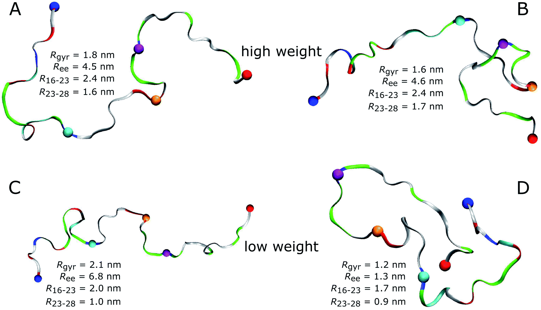 | ||
| Fig. 7 High-weight (A and B) and low-weight structures (C and D) determined by reweighting the a99SB-UCB trajectory using the Bayesian/maximum entropy technique.62 Aβ40 is shown as band and colored according to amino acid residue type (basic: blue, acidic: red, histidine: cyan, polar: green, hydrophobic: white). Following residues are indicated by spheres: N-terminus (blue), K16 (cyan), D23 (orange), K28 (mauve), C-terminus (red). The structures are characterized in terms of Ree, Rgyr, the K16–D23 distance (R16–23), and the D23–K28 distance (R23–28). | ||
The inspection of the corresponding structures for C36m (Fig. S20†) reveals a similar structural difference for the sequence 16KLVFFAE23 as seen for a99SB-UCB. While in the high-weight structures this sequence is rather extended, it exhibits a turn at F19/F20 in the low-weight structures. Thus, based on the J-couplings, a turn in that region should not be sampled. Apart from this turn, visual inspection failed to identify further major differences. In fact, the conformations in Fig. S20A and B† (high-weight structures) and those in Fig. S20C and D† (low-weight structures) look rather similar. As for a99SB-UCB it is observed that reweighting the structures does not change the distribution of Rgyr values much. Nonetheless, a small change of Rgyr to a lower average value is observed for C36m. This agrees with the finding that the 50 high-weight structures obtained with C36m are generally more compact (average Ree = 2.79 nm) than their low-weight counterparts (average Ree = 3.65 nm). This is accompanied by a smaller distance between D23 and K28 (0.97 nm vs. 1.24 nm) but a larger K16–D23 distance (2.11 nm vs. 1.90 nm). The conclusion is that, when a FF is not able to provide a generally satisfactory structural ensemble (as in the case of C36m), it might not be possible to optimize for different experimental observables at once; here, agreement with the J-couplings was optimized, which led to a larger disagreement for Ree.
If one wants to gain an in-depth understanding of the structural features sampled in the low-weight structures that are in disagreement with the various available experimental observables, it would be necessary to determine these observables for the low-weight structures (and also high-weight structures as reference) per residue and then correlate these with the structural preferences as (for instance) measured by the dihedral distribution in Ramachandran space. Based on this, suggestions for possible force field optimizations could be made. An alternative approach would be to employ an automatic reparametrization based on a Bayesian formalism that takes the available experimental data into account.62 However, considering that the recently attained excellent agreement between a9SB-UCB-simulated Aβ ensemble and experimental data has taken so long to achieve by the simulation research community, it is important that extreme care is taken in performing any reoptimization attempt. The goal should be to make as little changes as necessary in order to avoid losing of what has been achieved. A classical example is shown in the case of a99SB-disp where a force field optimization procedure that was too general and/or too extensive destroyed what had already been gained in a99SB-ILDN/TIP4P-D which for Aβ40 clearly performs better than its optimized a99SB-disp descendant.
4.3 How long should MD simulations of Aβ be?
The kinetic analysis of the seven 30-μs MD simulation does not only allow us to conclude which of the FFs provides the best structural ensemble of Aβ, but also how long standard MD simulations of Aβ should be if one aims for converged results of the structural ensemble. To answer this question we analyzed the convergence behavior of different quantities, such as the RMSD, number of clusters, secondary structure, Rgyr and also Ree, and calculated MSMs based on TICA for dimensionality reduction. The RMSD was identified as a useless measure to assess convergence for the simulation of an IDP like Aβ. If one aims for converged results for Rgyr and Ree it seems that for many of the FFs less than 10 μs of MD sampling is sufficient. A time limit below 10 μs has not been provided here since this was not analyzed in the present work. However, from FRET experiments of Aβ it was concluded that conformational dynamics leading to changes of the end-to-end distance does not exceed 1 μs.35 Thus, it might be that for this quantity a sampling time of 1 μs might even be sufficient. Yet with a03ws and a99SB-disp*-ILDN/TIP3P large changes in both Ree and Rgyr were still observed after 10 μs of MD. However, as both FFs were already identified as not suitable for modeling the structural ensemble of Aβ, in the following discussion we will ignore them. Though it is interesting to note that FFs, which fail to provide an acceptable description of the metastable states, also fail to reproduce the peptide kinetics. This is understandable as conformations in disagreement with experiment are also expected to be connected by transition states different from reality. Moreover, the Aβ conformations favored by these two FFs are overly stable in terms of intrapeptide contacts, which explains the slow kinetics generated with them.If one uses the secondary structure as a measure for convergence one also finds that 10 μs seem sufficient as the averages of the different structural elements did not change much beyond that time. However, the evolution of the secondary structure shows that for all FFs considerable changes in secondary structure can occur beyond 10 μs (which do not much affect the average values). Thus, the recommendation is to simulate Aβ for at least 10 μs, if possible longer. The same recommendation is made based on the cluster and MSM analyses. The number of clusters converged only beyond a sampling time of 10 μs, and for the best FF, a99SB-UCB, this was achieved only after 20 μs as a result of rare β-sheet formation. This observation agrees with those derived from the MSM analysis. Here, the MFPTs suggest that simulation times of ≳30 μs are even better as the transitions to rare states require sampling times of that length. As a final check we analyzed the convergence of the time-averaged Cα–Cα distances (Fig. S21†), an idea originating from testing for ergodicity in supercooled liquids76 and later applied to Aβ.77 Depending on how much Cα–Cα distance fluctuations one allows before one considers a simulation to be converged, one again finds that more than 20 or even 30 μs are needed for obtaining stable Cα–Cα distance averages.
Since the current simulations are limited to 30 μs, one might of course wonder whether completely new conformations would be sampled if the simulations were extended. Another valid question is whether simulating multiple shorter simulations would provide a better approach than sampling one long simulation. To answer these questions we compared our results to those obtained from running 5119 trajectories between 9.75 and 90.5 ns in length with an aggregated simulation time of 315 μs for Aβ42 modeled by C22*/TIP3P.78 The resulting MSM identified four states with similar populations and Aβ structures as obtained from our analysis, while several of the MFPTs are lower than those determined here (Fig. S22†). A likely explanation for this discrepancy is the lag time of only 12.5 ns used by Löhr et al.;78 for a number of other proteins it was shown that lag times ≲100 ns lead to an underestimation of the MFPTs derived from MSMs.79 Nonetheless, the comparison with the results obtained by Löhr et al. suggests that it is sufficient if one simulates monomeric Aβ for 30 μs, even when kinetically slow FFs like C22*/TIP3P and C36m are being employed. On the other hand, when we run 6 × 5 μs MD simulations of Aβ40 using a99SB-UCB and six different starting structures collected at t = 5, 10,…, 30 μs from the corresponding 30 μs MD simulation, the trajectories did not converge (Fig. S23†). In the one long simulation we observed two rare transitions from the random coil state to conformations with β-hairpins (also involving some α-helix), which are not sampled by the six shorter simulations, even though one starting structure of these extra simulations was already close to a β-hairpin. A future study therefore needs to investigate the different convergence behavior of one long versus multiple shorter simulations.
5 Conclusions
We analyzed the 30 μs MD simulations that were acquired for Aβ40 using seven different FF/water-model combinations by D. E. Shaw Research.32 One aim of our analysis was to assess how much of MD time is needed for obtaining fully converged MD ensembles for this peptide. Our analysis of the evolution of different structural quantities as well as Markov state models calculated from the MD data showed that the answer to this question partly depends on the FF used as the different FFs produced different kinetics for Aβ. Since only the FFs that are in agreement with experimental results should be employed, we calculated various NMR and FRET observables from the MD trajectories and compared the resulting values to the experimental ones.35,63 This comparison revealed that the best FF field for Aβ is a99SB-UCB, which is based on a99SB/TIP4P-Ew and includes LJ and dihedral modifications implemented by Head-Gordon and co-workers.33,34 The second best performance is found for a99SB-ILDN/TIP4P-D, which can also be recommended for modeling Aβ, while all other FFs showed severe failures in reproducing at least one, in most cases more sets of experimental quantities. Usage of a03ws and a99SB*-ILDN/TIP3P for Aβ simulations is clearly discouraged as they produce too much folded Aβ conformations, with too much helix in the case of a03ws and too much β-sheet with a99SB*-ILDN/TIP3P. The other three FFs under study, a99SB-disp, C22*/TIP3P, and C36m, produced acceptable results for Aβ![[thin space (1/6-em)]](https://www.rsc.org/images/entities/char_2009.gif) but considering that there are two FFs that clearly perform better, the recommendation is to use these.
but considering that there are two FFs that clearly perform better, the recommendation is to use these.
The MSMs resulting from the simulations with a99SB-UCB and a99SB-ILDN/TIP4P-D are both dominated by one state that harbors extended Aβ40 structures with little to none inter-residue contacts beyond direct neighbor contacts. Two further metastable, yet low-populated states (total population of 5%) are identified with both FFs, which involve β-hairpin formation. With a99SB-UCB the β-hairpins in both these states are centered at residues V24/G25 and involve contacts between F19/F20 with I31/I32. With a99SB-ILDN/TIP4P-D such β-hairpin is also sampled in one of the MSM states, while the other one contains a β-hairpin in the N-terminal region. Transitions to these low-populated states are rare events and most of them are thus associated with MFPTs reaching ≈30 μs or even more. The conclusion therefore is that at least 30 μs of MD sampling is needed to obtain converged trajectories producing the equilibrium distribution of Aβ conformations. This conclusion is supported by the analysis of the convergence of other structural quantities, such as the number of conformational clusters sampled.
Unlike the MFPTs to metastable states, the implied time scales derived from an MSM are a measure for intrapeptide reorientations. For these motions, an upper limit of 1 μs was predicted from different fluorescent spectroscopic measurements.35,36 Only for a99SB-UCB and a99SB-ILDN/TIP4P-D the slowest implied time scales are below 1 μs, while with all other FFs the kinetics of Aβ40 is predicted to be much slower, in the cases of a03ws, a99SB-disp and a99SB*-ILDN/TIP3P the slowest intrapeptide motions even reach time scales beyond 10 μs. Thus, also in terms of kinetics a99SB-UCB and a99SB-ILDN/TIP4P-D are the only two FFs in agreement with experiment. Nonetheless, even though the thermodynamics and kinetics of Aβ is modeled well with these two FFs, there is still further room for improvement. For instance, while a99SB-UCB is very good in reproducing NMR values for the C-terminal side of the peptide, this is less so the case for the region G9–H13. Thus, further FF improvements for Aβ should focus on this region, while keeping the level of quality for the rest of the peptide. Overall, a major step forward in terms of FF quality for Aβ has been reached with a99SB-UCB and also a99SB-ILDN/TIP4P-D. It will be interesting to see how the kinetics of Aβ oligomer formation and the resulting structures will look like when simulated with these FFs, i.e., when the aggregation process is initiated from extended, disordered, and not partly folded states as was the case due to FF bias in previous Aβ aggregation simulations.
Author contributions
A. P. and B. S. designed the computer simulations. A. P., S. S., M. A. and M. K. performed and analyzed the simulations. A. P., S. S. and B. S. wrote the manuscript. All authors contributed to discussing the results and reviewing the manuscript.Conflicts of interest
There are no conflicts to declare.Acknowledgements
The authors thank Ushnish Sengupta for fruitful discussions, Jennifer Loschwitz for helping to run some of the MD simulations, and Dr Olujide Olubiyi for proofreading the manuscript. M. K. and B. S. acknowledge funding for this project from the Palestinian-German Science Bridge financed by the German Federal Ministry of Education and Research (BMBF). Computing resources granted through JARA-HPC (project Amyloid-MSM) on the supercomputer JURECA at Forschungszentrum Jülich, RWTH Aachen University under project rwth0400, and the Centre for Information and Media Technology at Heinrich Heine University Düsseldorf are gratefully acknowledged. The funders had no role in study design, data collection and analysis, decision to publish, or preparation of the manuscript.Notes and references
- M. A. DeTure and D. W. Dickson, Mol. Neurodegener., 2019, 14, 32 CrossRef PubMed.
- S. H. Barage and K. D. Sonawane, Neuropeptides, 2015, 52, 1–18 CrossRef CAS PubMed.
- F. Chiti and C. M. Dobson, Annu. Rev. Biochem., 2017, 86, 27–68 CrossRef CAS PubMed.
- R. Tycko, Neuron, 2015, 86, 632–645 CrossRef CAS PubMed.
- L. Nagel-Steger, M. C. Owen and B. Strodel, ChemBioChem, 2016, 17, 657–676 CrossRef CAS PubMed.
- M. C. Owen, D. Gnutt, M. Gao, S. K. T. S. Wärmländer, J. Jarvet, A. Gräslund, R. Winter, S. Ebbinghaus and B. Strodel, Chem. Soc. Rev., 2019, 48, 3946–3996 RSC.
- I. Marsden, L. Minamide and J. Bamburg, J. Alzheimer's Dis., 2011, 24, 681–691 CAS.
- J. Nasica-Labouze, P. H. Nguyen, F. Sterpone, O. Berthoumieu, N.-V. Buchete, S. Coté, A. De Simone, A. J. Doig, P. Faller, A. Garcia, A. Laio, M. S. Li, S. Melchionna, N. Mousseau, Y. Mu, A. Paravastu, S. Pasquali, D. J. Rosenman, B. Strodel, B. Tarus, J. H. Viles, T. Zhang, C. Wang and P. Derreumaux, Chem. Rev., 2015, 115, 3518–3563 CrossRef CAS PubMed.
- B. Ahmad, Y. Chen and L. J. Lapidus, Proc. Natl. Acad. Sci. U. S. A., 2012, 109, 2336–2341 CrossRef CAS PubMed.
- L. J. Lapidus, Mol. BioSyst., 2013, 9, 29–35 RSC.
- Y. Xu, J. Shen, X. Luo, W. Zhu, K. Chen, J. Ma and H. Jiang, Proc. Natl. Acad. Sci. U. S. A., 2005, 102, 5403–5407 CrossRef CAS PubMed.
- O. O. Olubiyi and B. Strodel, J. Phys. Chem. B, 2012, 116, 3280–3291 CrossRef CAS PubMed.
- N. G. Sgourakis, Y. Yan, S. A. McCallum, C. Wang and A. E. García, J. Mol. Biol., 2007, 368, 1448–1457 CrossRef CAS PubMed.
- N. G. Sgourakis, M. Merced-Serrano, C. Boutsidis, P. Drineas, Z. Du, C. Wang and A. E. García, J. Mol. Biol., 2011, 405, 570–583 CrossRef CAS PubMed.
- A. K. Somavarapu and K. P. Kepp, ChemPhysChem, 2015, 16, 3278–3289 CrossRef CAS PubMed.
- S. R. Gerben, J. A. Lemkul, A. M. Brown and D. R. Bevan, J. Biomol. Struct. Dyn., 2014, 32, 1817–1832 CrossRef CAS PubMed.
- M. Carballo-Pacheco and B. Strodel, Protein Sci., 2017, 26, 174–185 CrossRef CAS PubMed.
- W. L. Jorgensen and J. Tirado-Rives, J. Am. Chem. Soc., 1988, 110, 1657–1666 CrossRef CAS PubMed.
- G. A. Kaminski, R. A. Friesner, J. Tirado-Rives and W. L. Jorgensen, J. Phys. Chem. B, 2001, 105, 6474–6487 CrossRef CAS.
- W. L. Jorgensen, J. Chandrasekhar, J. D. Madura, R. W. Impey and M. L. Klein, J. Chem. Phys., 1983, 79, 926–935 CrossRef CAS.
- V. Hornak, R. Abel, A. Okur, B. Strockbine, A. Roitberg and C. Simmerling, Proteins, 2006, 65, 712–725 CrossRef CAS PubMed.
- H. W. Horn, W. C. Swope, J. W. Pitera, J. D. Madura, T. J. Dick, G. L. Hura and T. Head-Gordon, J. Chem. Phys., 2004, 120, 9665–9678 CrossRef CAS PubMed.
- R. B. Best and G. Hummer, J. Phys. Chem. B, 2009, 113, 9004–9015 CrossRef CAS PubMed.
- K. Lindorff-Larsen, S. Piana, K. Palmo, P. Maragakis, J. L. Klepeis, R. O. Dror and D. E. Shaw, Proteins, 2010, 78, 1950–1958 CrossRef CAS PubMed.
- D.-W. Li and R. Brüschweiler, Angew. Chem., Int. Ed., 2010, 49, 6778–6780 CrossRef CAS PubMed.
- S. Piana, K. Lindorff-Larsen and D. E. Shaw, Biophys. J., 2011, 100, L47–L49 CrossRef CAS PubMed.
- S. Rauscher, V. Gapsys, M. J. Gajda, M. Zweckstetter, B. L. de Groot and H. Grubmüller, J. Chem. Theory Comput., 2015, 11, 5513–5524 CrossRef CAS PubMed.
- S. Piana, A. G. Donchev, P. Robustelli and D. E. Shaw, J. Phys. Chem. B, 2015, 119, 5113–5123 CrossRef CAS PubMed.
- W. Wang, W. Ye, C. Jiang, R. Luo and H.-F. Chen, Chem. Biol. Drug Des., 2014, 84, 253–269 CrossRef CAS PubMed.
- R. B. Best, W. Zheng and J. Mittal, J. Chem. Theory Comput., 2014, 10, 5113–5124 CrossRef CAS PubMed.
- J. Huang, S. Rauscher, G. Nawrocki, R. Ting, M. Feig, B. de Groot, H. Grubmüller and A. MacKerell, Nat. Methods, 2017, 14, 71–73 CrossRef CAS PubMed.
- P. Robustelli, S. Piana and D. Shaw, Proc. Natl. Acad. Sci. U. S. A., 2018, 115, 201800690 CrossRef PubMed.
- P. S. Nerenberg, B. Jo, C. So, A. Tripathy and T. Head-Gordon, J. Phys. Chem. B, 2012, 116, 4524–4534 CrossRef CAS PubMed.
- P. S. Nerenberg and T. Head-Gordon, J. Chem. Theory Comput., 2011, 7, 1220–1230 CrossRef CAS PubMed.
- F. Meng, M. M. Bellaiche, J. Y. Kim, G. H. Zerze, R. B. Best and H. S. Chung, Biophys. J., 2018, 870–884 CrossRef CAS PubMed.
- S. Acharya, K. Srivastava, S. Nagarajan and L. Lapidus, ChemPhysChem, 2016, 17, 3470–3479 CrossRef CAS PubMed.
- A. A. Watson, D. P. Fairlie and D. J. Craik, Biochemistry, 1998, 37, 12700–12706 CrossRef CAS PubMed.
- M. J. Abraham, T. Murtola, R. Schulz, S. Páll, J. C. Smith, B. Hess and E. Lindah, SoftwareX, 2015, 1–2, 19–25 CrossRef.
- G. Bussi, D. Donadio and M. Parrinello, J. Chem. Phys., 2007, 126, 014101 CrossRef PubMed.
- M. Parrinello and A. Rahman, J. Appl. Phys., 1981, 52, 7182–7190 CrossRef CAS.
- B. Hess, H. Bekker, H. J. Berendsen and J. G. Fraaije, J. Comput. Chem., 1997, 18, 1463–1472 CrossRef CAS.
- T. Darden, D. York and L. Pedersen, J. Chem. Phys., 1993, 98, 10089–10092 CrossRef CAS.
- D. Van Der Spoel, E. Lindahl, B. Hess, G. Groenhof, A. E. Mark and H. J. Berendsen, GROMACS: Fast, flexible, and free, 2005 Search PubMed.
- S. Pronk, S. Páll, R. Schulz, P. Larsson, P. Bjelkmar, R. Apostolov, M. R. Shirts, J. C. Smith, P. M. Kasson, D. Van Der Spoel, B. Hess and E. Lindahl, Bioinformatics, 2013, 845–854 CrossRef CAS PubMed.
- W. Humphrey, A. Dalke and K. Schulten, J. Mol. Graphics, 1996, 33–38 CrossRef CAS.
- N. Michaud-Agrawal, E. J. Denning, T. B. Woolf and O. Beckstein, J. Comput. Chem., 2011, 2319–2327 CrossRef CAS PubMed.
- R. T. McGibbon, K. A. Beauchamp, M. P. Harrigan, C. Klein, J. M. Swails, C. X. Hernández, C. R. Schwantes, L. P. Wang, T. J. Lane and V. S. Pande, Biophys. J., 2015, 1528–1532 CrossRef CAS PubMed.
- K. J. Bowers, E. Chow, H. Xu, R. O. Dror, M. P. Eastwood, B. A. Gregersen, J. L. Klepeis, I. Kolossvary, M. A. Moraes, F. D. Sacerdoti, J. K. Salmon, Y. Shan and D. E. Shaw, Proc. 2006 ACM/IEEE Conf. Supercomput. SC’06, 2006, p. 43 Search PubMed.
- X. Daura, K. Gademann, B. Jaun, D. Seebach, W. F. van Gunsteren and A. E. Mark, Angew. Chem., Int. Ed., 1999, 236–240 CrossRef CAS.
- D. Frishman and P. Argos, Proteins, 1995, 566–579 CrossRef CAS PubMed.
- M. K. Scherer, B. Trendelkamp-Schroer, F. Paul, G. Pérez-Hernández, M. Hoffmann, N. Plattner, C. Wehmeyer, J.-H. Prinz and F. Noé, J. Chem. Theory Comput., 2015, 11, 5525–5542 CrossRef CAS PubMed.
- M. K. Scherer, B. E. Husic, M. Hoffmann, F. Paul, H. Wu and F. Noé, J. Chem. Phys., 2019, 150, 194108 CrossRef PubMed.
- G. Pérez-Hernández, F. Paul, T. Giorgino, G. De Fabritiis and F. Noé, J. Chem. Phys., 2013, 139, 015102 CrossRef PubMed.
- R. Campello, D. Moulavi and J. Sander, Advances in Knowledge Discovery and Data Mining, PAKDD, 2013, Lecture Notes in Computer Science, 2013, pp. 160–172 Search PubMed.
- S. Kube and M. Weber, J. Chem. Phys., 2007, 126, 024103 CrossRef PubMed.
- S. Röblitz and M. Weber, Adv. Data Anal. Classi., 2013, 7, 147–179 CrossRef.
- J.-H. Prinz, H. Wu, M. Sarich, B. Keller, M. Senne, M. Held, J. D. Chodera, C. Schütte and F. Noé, J. Chem. Phys., 2011, 134, 174105 CrossRef PubMed.
- Y. Shen and A. Bax, J. Biomol. NMR, 2010, 13–22 CrossRef PubMed.
- M. Karplus, J. Chem. Phys., 1959, 11–15 CrossRef CAS.
- B. Vögeli, J. Ying, A. Grishaev and A. Bax, J. Am. Chem. Soc., 2007, 9377–9385 CrossRef PubMed.
- J. Lincoff, S. Sasmal and T. Head-Gordon, J. Chem. Phys., 2019, 150, 104108 CrossRef PubMed.
- S. Bottaro, T. Bengtsen and K. Lindorff-Larsen, in Integrating Molecular Simulation and Experimental Data: A Bayesian/Maximum Entropy Reweighting Approach, ed. Z. Gáspári, Springer US, New York, NY, 2020, pp. 219–240 Search PubMed.
- J. Roche, Y. Shen, J. H. Lee, J. Ying and A. Bax, Biochemistry, 2016, 55, 762–775 CrossRef CAS PubMed.
- D. Wishart and D. Case, Methods Enzymol., 2001, 338, 3–34 CAS.
- M. Kjaergaard and F. Poulsen, J. Biomol. NMR, 2011, 50, 157–165 CrossRef CAS PubMed.
- M. Kjaergaard, S. Brander and F. Poulsen, J. Biomol. NMR, 2011, 49, 139–149 CrossRef CAS PubMed.
- A. B. Mantsyzov, A. S. Maltsev, J. Ying, Y. Shen, G. Hummer and A. Bax, Protein Sci., 2014, 23, 1275–1290 CrossRef CAS PubMed.
- A. Mantsyzov, Y. Shen, J. Lee, G. Hummer and A. Bax, J. Biomol. NMR, 2015, 63, 85–95 CrossRef CAS PubMed.
- R. Best, N.-V. Buchete and G. Hummer, Biophys. J., 2008, 95, L07–L09 CrossRef CAS PubMed.
- D. Chakraborty, J. Straub and D. Thirumalai, Proc. Natl. Acad. Sci. U. S. A., 2020, 202002570 Search PubMed.
- D. Granata, F. Baftizadeh, J. Habchi, C. Galvagnion, A. De Simone, C. Camilloni, A. Laio and M. Vendruscolo, Sci. Rep., 2015, 5, 15449 CrossRef CAS PubMed.
- M. Nygaard, B. B. Kragelund, E. Papaleo and K. Lindorff-Larsen, Biophys. J., 2017, 113, 550–557 CrossRef CAS PubMed.
- N. Rezaei-Ghaleh, G. Parigi and M. Zweckstetter, J. Phys. Chem. Lett., 2019, 10, 3369–3375 CrossRef CAS PubMed.
- S. Jephthah, L. Staby, B. B. Kragelund and M. Skepö, J. Chem. Theory Comput., 2019, 15, 2672–2683 CrossRef CAS PubMed.
- A. H. Larsen, Y. Wang, S. Bottaro, S. Grudinin, L. Arleth and K. Lindorff-Larsen, PLoS Comput. Biol., 2020, 16, 1–29 CrossRef PubMed.
- D. Thirumalai and R. D. Mountain, Phys. Rev. E, 1993, 47, 479–489 CrossRef PubMed.
- K. A. Ball, A. H. Phillips, P. S. Nerenberg, N. L. Fawzi, D. E. Wemmer and T. Head-Gordon, Biochemistry, 2011, 50, 7612–7628 CrossRef CAS PubMed.
- T. Löhr, K. Kohlhoff, G. Heller, C. Camilloni and M. Vendruscolo, Nature Comput. Sci., 2021, 1, 71–78 CrossRef.
- E. Suárez, R. Wiewiora, C. Wehmeyer, F. Noé, J. Chodera and D. Zuckerman, bioRxiv, 2020 DOI:10.1101/2020.11.09.374496.
Footnotes |
| † Electronic supplementary information (ESI) available. See DOI: 10.1039/d0sc04657d |
| ‡ These authors contributed equally. |
| § Current address: LifeGlimmer GmbH, Markelstraβe 38, 12163 Berlin, Germany. |
| This journal is © The Royal Society of Chemistry 2021 |