 Open Access Article
Creative Commons Attribution 3.0 Unported Licence
Design of dynamic trajectories for efficient and data-rich exploration of flow reaction design spaces†
Federico
Florit
 ab,
Anirudh M. K.
Nambiar
a,
Christopher P.
Breen
c,
Timothy F.
Jamison
 c and
Klavs F.
Jensen
 *a
*a
aMassachusetts Institute of Technology, Department of Chemical Engineering, Cambridge, MA 02139, USA. E-mail: kfjensen@mit.edu
bPolitecnico di Milano, Dipartimento di Chimica, Materiali e Ingegneria Chimica “G. Natta”, Piazza Leonardo da Vinci, 32, 20133, Milano, Italy
cMassachusetts Institute of Technology, Department of Chemistry, Cambridge, MA 02139, USA
First published on 21st September 2021
Abstract
Batch and continuous reactors both enable exploration of a chemical design space. The former rely on transient experiments, thus experiencing a wide variety of operating conditions over time, whereas the latter are usually operated at steady state and are representative of only one set of conditions. Operating a continuous reactor under dynamic conditions allows more efficient exploration of the underlying reaction space for extraction of kinetics and optimization of performance. We present a methodology to efficiently explore a design space using a tubular flow reactor installed on an automatic platform (equipped with FTIR and HPLC analysis) operated in a transient regime using sinusoidal variations of the parameters. This data-dense method proves to be quicker with respect to steady-state operations because of the larger amount of information collected during a single experiment. A computational analysis provides a simple criterion for the design of dynamic experiments in order for them to be representative of steady-state conditions. The methodology is applied experimentally to the synthesis of a pharmaceutical intermediate via an esterification reaction in the presence of base. In the experiments, up to three parameters (reaction time, base equivalents, and temperature) are changed simultaneously. Proper design of the trajectories in the design space allows verification of the consistency of the results by exploiting the self-crossings within each trajectory and crossings between different trajectories. The experiments further validate the developed criterion for dynamic operations.
1 Introduction
Development of new syntheses and performance enhancement of existing processes continue to be challenges for production of both fine-chemicals and commodities. Classical engineering approaches usually involve the repeated use of lab-scale reactors at under different conditions to make a model of the reaction based on a hypothesized mechanism and extracted kinetic parameters. The resulting model can subsequently be used to maximize some objective (e.g., yield or productivity) over feasible reaction conditions. This method is very effective as it gives good insight on the underlying chemistry and physics of the studied reaction, but it requires extensive experimental efforts and good understanding of the actual reaction mechanism.One way to reduce the number of experiments required to find an optimal condition is the use of design of experiment (DoE) methods,1,2 which provide reaction conditions aimed at describing the variations of some objective function with respect to the optimization parameters while using a small number of experiments. These approaches employ a simple model, the response surface, to represent the objective function (e.g., yield) by parameters that link the objective function to the optimization variables (e.g., reaction temperature, contact time, and reagent concentration).3,4 Thus, these methods rely on the response surface providing a good approximation the actual system.
Tubular reactors used in flow chemistry typically have very low dispersion, and thus, operate as plug-flow reactors (PFRs).5,6 For such systems the residence time distribution is narrow and represented by the average residence time, while fluid properties (e.g., composition and temperature) are uniform across the section of the reactor. The continuous reactor can then be represented as a sequence of batch reactors (BRs) moving in space, the segregated model.5 A batch reactor enters the system at some time and leaves the reactor after a time interval equal to the average residence time, thus the residence time corresponds to the reaction time of the batch reactor. The initial conditions for each BRs correspond to the inlet boundary conditions of the continuous reactor. When the continuous reactor is operated dynamically, i.e., residence time and inlet conditions change in time, the batch reactors experience different reaction times and initial conditions. In contrast, a continuous system at steady state represents only one set of initial conditions (one equivalent batch reactor). Different reaction conditions are attained along the reactor, but it is difficult to obtain information from these intermediate points of the steady system due to geometrical, mechanical, and optical difficulties in accessing the flow path.7
Steady-state conditions are generally used in the DoE-based methods, which discard the information gathered during the change of reaction conditions (the transient behavior of the reactor). The dynamic (transient) regime of a reactor is therefore richer in information provided to the user compared to steady-state methods. The larger amount of information provided by a single dynamic experiment has been exploited in several kinetic studies in which the reaction outcomes were monitored for varying residence times.7–9 Hone et al.10 have shown that the approach can be extended to account for the effect of axial dispersion, and Aroh and Jensen11 have explored effects of two simultaneous variations of parameters with time exemplified by linear variations of flowrate and temperature. Most recently, Taylor et al.12 have used linear ramps of flowrate at discrete temperatures combined with machine learning to discriminate among reaction mechanisms. All the aforementioned experimental studies required inline/online analysis of the reactor effluent, such as FTIR,8,11 Raman,7,9 HPLC,10,12 and NMR.13
A tubular reactor with low dispersion operated in a dynamic regime allows exploration of the effects of different variables on reactor performance as they change over time, resulting in a powerful tool for chemical design space exploration and eventually (dynamic) optimization. Wyvratt et al.14 used dynamic experiments to explore a design space for a chemical reaction (Knoevenagel condensation) by linearly changing (one at a time) the residence time and the catalyst equivalents with time, using an online FTIR. The parameters were also changed together in a linear orthogonal fashion, as suggested by other researchers,11 or using sinusoidal variations for one parameter and linear variations for the other. A response surface was fitted to the obtained dynamic data which are in good agreement with the steady-state results. Haas et al.15 have adopted a similar concept to study the chemical design space of a photochemical cycloaddition reaction, where the parameters investigated were reaction time and one reactant concentration. In this case the residence time was changed by using multiple step changes of the inlet flowrate. An online HPLC/MS system was used for the analysis. The concept of transient flow experiments is an extension of batch dynamic experiments, for which the aim is to obtain a trajectory of the optimization parameters in order to optimize some performance function.16–18 While batch reactors optimized in such a way are then operated with dynamic variations even after obtaining the optimal conditions, continuous reactors optimized using dynamic experiments are run at constant conditions (those obtained dynamically at the optimal conditions).
Herein we develop experimental design rules for dynamic exploration of the chemical design space for a reaction performed in a continuous reactor. These experimental design rules are model-free, thus not require estimating a response surface or any information regarding the kinetics of the system. Using the synthesis of a pharmaceutical intermediate as a case study, the resulting methods demonstrate the feasibility of using dynamic experiments, specifically sinusoidal variations, to explore chemical reaction space on an automated flow chemistry platform.19
2 Mathematical model
2.1 Input reconstruction
In a continuous reactor operated at steady-state, the outlet variables (such as conversion and yield) are determined by the inlet variables (such as concentration and flowrate) which remain constant in time. During a dynamic experiment the inlet variables change over time. The outlet variables at time t are determined by the inlet variables imposed at time t − τ, τ being the effective residence time of the equivalent batch reactors of the segregated model. The residence time changes with time as the total inlet flowrate varies. We assume that the system is homogeneous with a constant and uniform density, which is a good approximation for homogeneous liquid-phase reactions, and all changes start at time t = 0, when the system is at steady state. Under such hypothesis it is possible to define the instantaneous residence time, τI, as: | (1) |
 | (2) |
 | (3) |
For changing variables that are not pointwise (determined solely at the inlet), but involve the entire reactor (such as the reactor temperature in general or the light intensity/wavelength for photochemical reactions), the BRs traveling inside the continuous system experience a range of such variables in time. If these variables do not change widely over the effective residence/reaction time, then they can be represented by averaged values.
2.2 Optimal dynamics
The variables to be explored for a given synthesis can be changed in any manner over time. Nevertheless, these variations should be realized in such a way that the results of the dynamic experiment represent the steady states of the process under the same conditions. The chemical species composition inside the reactor (which will eventually determine some outlet variable, e.g., yield) should thus be similar to the one observed at steady state. The discrepancy between the observed result during the dynamic experiment and the steady state could result from the non-negligible dispersion of a real system20 and the intrinsic dynamics of the system.By means of mass balance equations, the concentration in the tubular reactor can be modeled using dimensionless quantities (details in the ESI†) describing how the dimensionless concentration of species i, ĉi (concentration divided by total initial inlet concentration), changes along the axial dimensionless coordinate, ![[x with combining circumflex]](https://www.rsc.org/images/entities/i_char_0078_0302.gif) (position divided by reactor length), and over the dimensionless time,
(position divided by reactor length), and over the dimensionless time, ![[t with combining circumflex]](https://www.rsc.org/images/entities/i_char_0074_0302.gif) (time divided by initial residence time). In order for the dynamic experiment to be representative of steady states, ∂ĉi/∂
(time divided by initial residence time). In order for the dynamic experiment to be representative of steady states, ∂ĉi/∂![[t with combining circumflex]](https://www.rsc.org/images/entities/i_char_0074_0302.gif) ≈ 0, i.e. the system is in a pseudo-steady state (PSS). The dimensionless concentration is determined by the intrinsic properties of the system (reaction kinetics and reactor properties) and the dynamics of the dimensionless parameters, ŷk (value of the parameter divided by its initial value), to be explored. ŷk thus represents how the considered parameter varies with respect to its initial value. Consequently the PSS condition is reached when:
≈ 0, i.e. the system is in a pseudo-steady state (PSS). The dimensionless concentration is determined by the intrinsic properties of the system (reaction kinetics and reactor properties) and the dynamics of the dimensionless parameters, ŷk (value of the parameter divided by its initial value), to be explored. ŷk thus represents how the considered parameter varies with respect to its initial value. Consequently the PSS condition is reached when:
 | (4) |
![[t with combining circumflex]](https://www.rsc.org/images/entities/i_char_0074_0302.gif) ≈ 0, which in practice means that
≈ 0, which in practice means that | (5) |
 is some (small) value below which the variations of parameter yk are deemed sufficiently small. This criterion for the optimal choice of the system dynamics can be seen as the intuitive need to have slow variations in time for all parameters in order for a dynamic system to represent a steady state. Therefore, steep changes of parameters (such as step changes with time) would not satisfy this condition, which could be an explanation for discrepancies observed between dynamic and steady experiments. Eqn (5) represents an a priori criterion for the design of dynamic experiments once the value of
  is known.
In this work sinusoidal changes are considered for all variables, which implies:
 | (6) |
 | (7) |
 can be determined by simulations of real systems during dynamic experiments and subsequent comparisons of the values of the objective function to those obtained at steady state under the same conditions. Several typical kinetic schemes with selectivity issues were considered (details in ESI†) and the objective function chosen was the yield of the product. Differences in yield, Δ, between the dynamic simulation value and the corresponding value obtained at steady state were evaluated for a wide range of kinetic parameters and sinusoidal variation parameters. In the simulations, the studied parameters varied at the same time were residence time, concentration ratio of the reactants, and temperature. The large number of simulations over comprehensive ranges of kinetic/process parameters allowed us to draw statistical conclusions regarding the value of Kyk from which a threshold
  could be set in order to have small values of Δ (small deviations from steady state). The simulated system is a series of a stirred reactor and a tubular reactor (similarly to the system used in the experiments). In the simulations the volume ratio between the two reactors was fixed, but it was observed that the influence of such ratio is modest if the mixed reactor is small compared to the tubular reactor, meaning that the former acts only as a mixing chamber. The molecular Peclet number ranged in the simulations between 1 × 101 and 2 × 10² to account for a small axial dispersion in the reactor, while the Damköhler number ranged between 3 × 10⁻¹² and 6 × 10⁶ (further details are provided in the ESI†). This initial evaluation involved 10
![[thin space (1/6-em)]](https://www.rsc.org/images/entities/char_2009.gif) 000 simulations running for approximately 9 hours on a 40-core (Intel Xeon Gold 6148 2.4 GHz) computer. The range of the dynamic and process variables was selected in order to take into account almost any practical conditions typical of flow chemistry reactions and conditions. A subset of the selected ranges would provide less stringent values of
000 simulations running for approximately 9 hours on a 40-core (Intel Xeon Gold 6148 2.4 GHz) computer. The range of the dynamic and process variables was selected in order to take into account almost any practical conditions typical of flow chemistry reactions and conditions. A subset of the selected ranges would provide less stringent values of  but would suffer from a sampling bias, with a loss of generality.
3 Experimental method
3.1 Materials and analysis
Chemicals were sourced from AK Scientific Inc. (Union City, CA), Sigma-Aldrich (St. Louis, MO), and Toronto Research Chemicals (Toronto, ON) and used as provided without further purification. 2-Bromo-N,N-dimethylacetamide 2 (97%, product # Z4866) and 4-hydroxyphenylacetic acid 1 (98%, product # A096) were purchased from AK Scientific. N,N-Diisopropylethylamine (99.5%, product # 387649) and N,N-dimethylacetamide (99.8%, anhydrous, product # 271012) were purchased from Sigma-Aldrich. An authentic sample of 2-(dimethylamino)-2-oxoethyl 2-(4-hydroxyphenyl)acetate 3 (99%, product # H807800) was purchased from Toronto Research Chemicals.Reagent solutions were prepared using volumetric glassware and N,N-dimethylacetamide (DMA) as the solvent, except for N,N-diisopropylethylamine which was used neat. Infrared spectroscopy data was collected using a Mettler Toledo FlowIR instrument in 15 second sampling intervals and processed using the iC IR 7.0 software by subtraction of the pure solvent spectrum. Calibration of 3 by was performed by injecting standard solutions into the flow cell such that the observed signal heights correlated linearly with concentration. A single point baseline with 1834 cm−1 as reference was applied to the in situ IR data. The height of the newly formed ester bond in 3 was observed in the range of 1783–1746 cm−1. Concentration of 3 was then computed by referencing the calibration curve.
High-performance liquid chromatography data was acquired using an Agilent 1260 Infinity series HPLC instrument equipped with an Agilent Poroshell 120 SB-C18 2.7 μm (3.0 × 50 mm) column (Agilent part # 689975-302T). The analytical method used in this study utilised a water (+0.1 v/v% formic acid) and acetonitrile (+0.1 v/v% formic acid) gradient. From 0–3.3 minutes, acetonitrile was increased from 5 to 100 v/v% followed by a hold at 100 v/v% acetonitrile from 3.3–5 minutes. At 5 minutes, acetonitrile was dropped back down to 5 v/v% and the column was re-equilibrated from 5–8 minutes. Starting material 1 and product 3 eluted at 1.7 and 2 minutes, respectively.
3.2 Experimental procedure
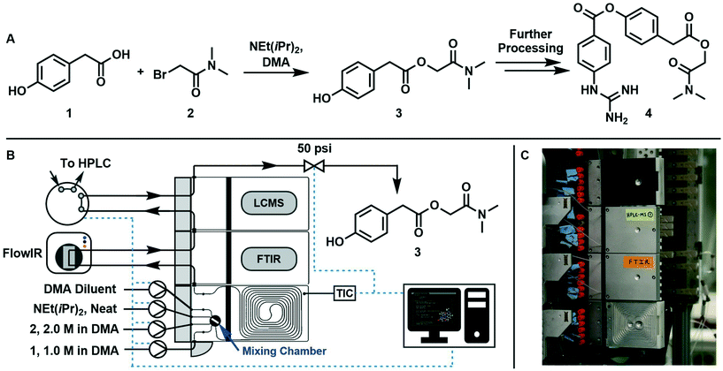
The synthesis of 2-(dimethylamino)-2-oxoethyl 2-(4-hydroxyphenyl)acetate (3, an intermediate in the synthesis of camostat 4, a serine protease inhibitor) can be run at temperatures above 40 °C in homogeneous conditions using DMA as solvent, starting from 1 and 2 with NEt(iPr)2·HBr as a by-product, following the scheme reported in Fig. 1A.The reaction was run in a 1 mL tubular reactor module of a plug-and-play automated flow chemistry platform previously reported by our lab19 (Fig. 1B and C). Inlet streams were pumped into the reactor using positive displacement pumps (VICI Valco Instruments, model M6HP, part # CP2-4111-DHP) and all lines had check valves (IDEX Health & Science, part # CV-3301). The reactor module contains a 0.125 mL pre-mixing chamber made of blow formed perfluoroalkoxy alkane (PFA) polymer film equipped with a magnetic stir bar. The mixed streams flow into a 1m tubular reactor (PFA tubing, 1/32′′ ID, 1/16′′ OD) that is pressed into channels in a heated aluminum housing which is kept at a set temperature with controlled electrical heating. The reactor effluent then passes through two inline analytical modules in series: an FTIR module connected to the inline Mettler Toledo FlowIR and an HPLC module connected to an online sample injection valve (VICI Valco Instruments, part # EUHB-CI6WHC.06) that injects a 60 nL sample of the reaction mixture into the Agilent HPLC every 10 minutes. Finally, the outlet module directs the effluent to a back-pressure regulator (Zaiput Flow Technologies, part # BPR-10) and then to waste. A graphical user interface built using Python's Tkinter package served three purposes: (i) interfacing with the reactor, pumps, and injection valve using serial communication, (ii) allowing the user to enter the parameters in eqn (6) that fully define the dynamic trajectory for each variable, and (iii) automatically generating flow rate and temperature trajectories and dynamically updating setpoints once the experiment is started.
The variables to be explored were the residence time inside the reactor, the mole equivalents of base with respect to 1, and temperature. The design space studied was: instantaneous residence time, τI, between 0.5 and 10 min, base equivalents (ratio between Hünig's base and 1 inlet concentration) between 1![[thin space (1/6-em)]](https://www.rsc.org/images/entities/char_2009.gif) :
:![[thin space (1/6-em)]](https://www.rsc.org/images/entities/char_2009.gif) 0 and 1
0 and 1![[thin space (1/6-em)]](https://www.rsc.org/images/entities/char_2009.gif) :
:![[thin space (1/6-em)]](https://www.rsc.org/images/entities/char_2009.gif) 3, and temperature, T, between 40 and 100 °C. 1 and 2 were always fed in stoichiometric quantities. Base equivalents were lowered by decreasing the base flow rate and increasing the DMA diluent flow rate by the same amount, allowing us to modulate base equivalents without altering the concentrations of 1 and 2.
3, and temperature, T, between 40 and 100 °C. 1 and 2 were always fed in stoichiometric quantities. Base equivalents were lowered by decreasing the base flow rate and increasing the DMA diluent flow rate by the same amount, allowing us to modulate base equivalents without altering the concentrations of 1 and 2.
Initially, two runs with constant temperature were performed by changing residence time and base equivalents. Afterwards, a run changing all variables at the same time was performed. All variations were sinusoidal in time as from eqn (6) and the parameters of average value, variation amplitude, and period are reported in Table 1, which also reports the experiment duration, texp. In order to ensure that the reaction mixture remained a liquid, the back-pressure regulator was set to 50 psi. Changes in residence time and base equivalents over time were realized by manipulating the flow rate of reactants and solvent with time.
| Run | t exp [min] | y k | y 0 k | δ y k | T y k [min] | K y k |
|---|---|---|---|---|---|---|
| 1 | 180 | τ I | 0.5 min | 19 | 360 | 0.17 |
| B.E. | 1.15 | 0.13 | 60 | 0.0068 | ||
| T | 333.15 K | 0 | — | 0 | ||
| 2 | 180 | τ I | 0.5 min | 19 | 360 | 0.17 |
| B.E. | 1.15 | 0.13 | 60 | 0.0068 | ||
| T | 353.15 K | 0 | — | 0 | ||
| 3 | 300 | τ I | 5.25 min | −0.9048 | 75 | 0.40 |
| B.E. | 1.15 | 0.13 | 60 | 0.072 | ||
| T | 313.15 K | 0.1916 | 600 | 0.011 |
The system was primed with solvent, brought to the initial reaction temperature, and a blank IR spectrum was acquired. A steady state condition was obtained with the parameters computed at t = 0, by waiting a time equal to three initial residence times (3τI(0)), and verifying the constant output through the IR spectra. Afterwards, the dynamic (transient) experiment was started for the duration reported in Table 1. The FTIR and HPLC data were collected starting from t = 0 at constant time intervals. Afterwards a new steady state condition was reached at the final values of the explored parameters. Further details on the experimental procedure are reported in the ESI.†
Sinusoidal variations were chosen in order to scan the parameters space in a smooth way allowing many combination of variables (high, low, intermediate values). Additionally, by adopting proper values of Tyk, one can design the variations in such a way that the same conditions (the same parameters) are obtained at different times (creating a crossing in the parameters space). If the same value of the objective function is obtained at the crossing, then the value obtained is path-independent (as it is approached from different directions in the parameters space) and this can only happen at a steady state. Thus the check of the objective function at a parameter crossing is an a posteriori check of the proper design of dynamic experiments.
4 Results
4.1 Simulations help define conditions for the dynamic exploration
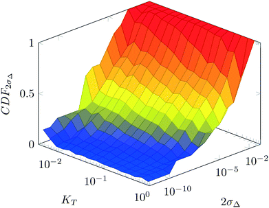
For various sets of kinetic/process parameters, a dynamic experiment was simulated (details in the ESI†) to obtain the objective function (yield) value over time and 50 random times were selected for comparison with the corresponding steady-state values of the objective function by computing the difference Δ of such values. The value of twice the standard deviation of the obtained distribution of Δ, 2σΔ, was selected as a representative figure for the comparison of steady states and dynamic simulation results. A distribution of 2σΔ is obtained by repeating its evaluation for many kinetic/process parameters. This distribution is a function of the computed values of Kyk. For the sake of example, the cumulative distribution function (CDF) of 2σΔ is plotted as a function of KT in Fig. 2.The CDF becomes skewed towards larger values of KT, while it broadens for smaller values of KT. This means, as expected, that slower variations (small Kyk) lead to results of the dynamic experiment that coincide with steady states. The threshold value  can be selected by choosing a limiting value of 2σΔ and a value of the CDF Kyk. The limit value of 2σΔ is selected to be equal to 0.01, while the value of the CDF to 0.90, meaning that
  guarantees yield deviations (between dynamic and steady simulations) below 1% in at least 90% of the cases possible in practice. As a consequence, the values of
  to be used in eqn (7) for residence time, concentration, and temperature can be computed for sinusoidal variations:
| Kmaxτ = 0.2, Kmaxc = 0.2, KmaxT = 0.04 | (8) |
4.2 Exploration of the chemical design space
After running each experiment, the dynamic output was collected both from FTIR and HPLC. By adopting suitable calibration curves the output signals were converted to concentration and finally to yield of the desired product (3). The set of input parameters (τI, base equivalents, and T) which generated a particular output in time was reconstructed by means of eqn (3), where the instantaneous residence time used takes into account additional volumes due to connections between the different parts of the equipment and the mixing chamber. In the following results the residence time reported (both instantaneous and effective) is referred to the tubular reactor only (excluding the connections between reactor and FTIR/HPLC equipment).Fig. 3 reports the time values of the studied parameters of run 1 from Table 1. The instantaneous residence time was varied with half a sinusoidal oscillation, while base equivalents with three full oscillations (see Fig. 3a), consequently the flowrate of each reactant and solvent changes non-sinusoidally in time (Fig. 3b). The yield measured with time is reported in Fig. 3c, which outlines the effect of both residence time and base equivalents variations.
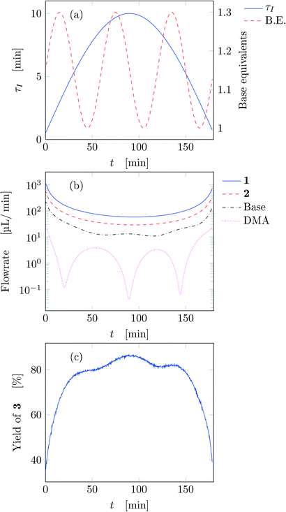 | ||
| Fig. 3 Time variation of the input and output parameters for run 1 of Table 1: (a) instantaneous residence time and base equivalents; (b) species flowrate; (c) measured yield of the desired product. | ||
Fig. 4a reports trajectory in design space. The space is bi-dimensional as only two parameters were changed sinusoidally in time, thus yield of 3 can be easily observed in Fig. 4b as a function of the two input parameters. The use of sinusoidal variations allowed two crossings in the parameter space (black circles in Fig. 4): the yield at these locations is the same on both path portions (as seen from the value of the yields), therefore all the points plotted represent steady-states of the system at the corresponding values of τ and base equivalents.
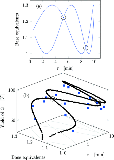 | ||
| Fig. 4 Results for run 1 of Table 1: (a) design space; (b) yield as a function of the design space parameters (circles: FTIR; squares: HPLC). The crossings of the trajectory are circled. | ||
The best reaction conditions obtained, for this particular temperature, are located at the extreme of the design space, namely at large τ and base equivalents. The large number of data collected via IR allowed checking the progress of the dynamic experiment and the HPLC data confirmed the location of the best conditions. It must be noted that the IR yields were systematically higher than the HPLC yields by approximately 5% due to overlap between the peaks of reactant 1 and product 3 in the IR spectrum which increased the product height. Nevertheless, the same yield trends were observed in both the IR and HPLC data. While IR enabled densely mapping out the design space along the trajectory, HPLC was a crucial complementary tool for providing the ground truth yield.
Fig. 5 reports the time behavior of the parameters of run 3 from Table 1. The instantaneous residence time undergoes four full oscillations, while base equivalents five (Fig. 5a), thus again, the flowrates do not follow sinusoidal variations (Fig. 5b). Temperature is varied by half an oscillation (Fig. 5c). The collected yield is depicted in Fig. 5c, where larger variations are observed mainly as a consequence of the residence time variations (lower residence time correspond to lower yields). The phase space is three-dimensional, thus it can be plotted in Fig. 6 as a 3D graph where yield can be reported as color of the various points. Note that the temperature reported is the integral average of the temperatures observed by the fluid during the residence time. Again, the large number of IR data collected allows to find a good indication of the optimal values of the parameters for this synthesis and the location of the best conditions studied is at the extrema of the analyzed space, namely, large residence time, base equivalents and temperature.
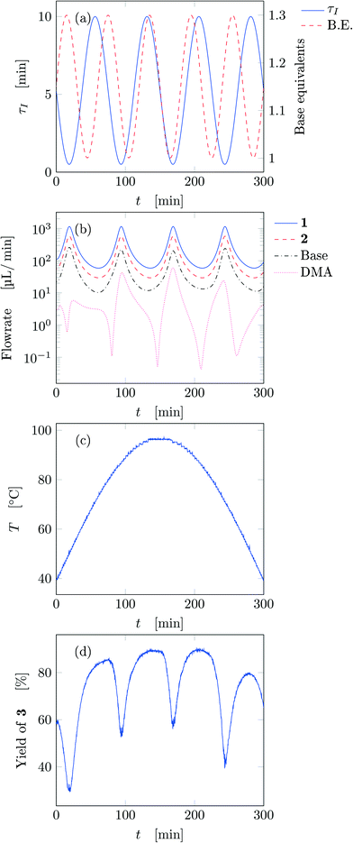 | ||
| Fig. 5 Time variation of the input and output parameters for run 3 of Table 1: (a) instantaneous residence time and base equivalents; (b) species flowrate; (c) measured temperature; (d) measured yield of the desired product. | ||
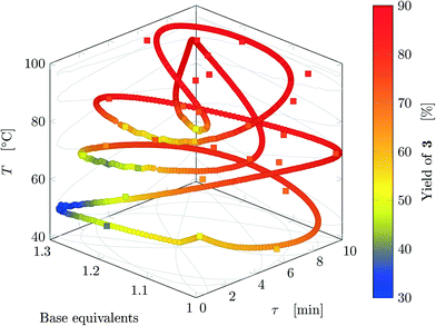 | ||
| Fig. 6 Results for run 3 of Table 1: design space where yield is represented by the color (circles: FTIR; squares: HPLC). This trajectory has no crossings. | ||
The sinusoidal variations allowed efficient exploration of the parameters space. Variations were chosen in order to collect more data closer to the expected location of the optimal conditions (in fact the region at low temperature and residence time was excluded), as inferred from runs 1 and 2. In the studied case, yield increases monotonically at increasing values of the three parameters in the analyzed space, but base equivalents do not change yield significantly at large values of residence time and temperature.
Results from the three experiments are combined in Fig. 7. The three experiments cross each other at three locations (marked on the figure), where the measured yield differs by approximately 1%, confirming that the dynamic experiment is able to describe steady states (as parameter crossings lead to the same result). Therefore, an a posteriori check of the choice of the dynamic variations can also be performed between intersecting experiments with different input parameters.
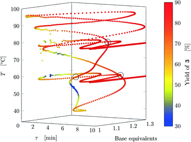 | ||
| Fig. 7 Design space where yield is represented by the color (data from FTIR) where all experiments are reported. The crossings between different experiments are circled. | ||
The developed methodology reduces dramatically the experimental effort and especially time to explore the design space. In steady-state experimental campaign, the same amount of information (same number of data-points for all three experiments) would have been obtained in approximately 270 h of experiments (considering just one residence time to reach steady-state and no cleaning times) compared to 11 h for the dynamic approach. In practice, at least three residence times are needed to ensure steady state and flushing procedures might also be performed in-between experiments, further increasing the experimental time. Thus, the dynamic experiments with the proposed methodology provide more than 75 times information than steady-state methods in the same time period. Finally, the task of manually preparing the exploration trajectory in the design space takes approximately the same time as manually preparing a DoE, thus becoming a negligible time compared to experimental time (both methods could be automatized). An additional advantage is that the trajectory designed in one design space can be easily transposed to any other design space with the same dimensions, and the trajectory will have roughly the same shape of the original one.
It is worth noting that the parameters chosen for experiments 1 and 2 lead to values of Kyk (see Table 1) satisfying the criteria obtained numerically, namely eqn (8). This confirms that slow variations satisfying eqn (7) lead to a dynamic response that is representative of steady states with very small deviations in yield. Run 3 does not satisfy the criterion for τ, nonetheless the experiment led to acceptable results (dynamic experiment coincident with steady states). The criteria developed are quite stringent as they allow a maximum yield deviation of 1%. If instead a 2% yield deviation is deemed acceptable, the values to be used in eqn (7) are:
| Kmaxτ = 0.6, Kmaxc = 0.5, KmaxT = 0.09 | (9) |
5 Conclusions
A model-free method for chemical design space exploration was developed using a continuous reactor in an automated platform operated in transient mode. Rules for the design of dynamic experiments were determined from a parametric analysis in order to make the results obtained with a (slow) transient experiment coincident with those achieved at steady state at the same operating conditions. The proposed criteria allow an a priori determination of the experimental deviation of the results obtained with the transient experiment with respect to steady state.The method was validated experimentally by studying the yield of an esterification reaction between a carboxylic acid and an alkyl halide. Small deviations (below 1%) from the steady-state yield of the desired product were obtained with the dynamic experiment if the proposed criteria are followed. Notably, no detailed information on the system studied (such as the kinetic mechanism and the physical–chemical properties) was required to apply the proposed method. The data-rich exploration of the design space further enabled identification of the best reaction conditions with a great reduction of experimental time in comparison with methods using steady states. This method could become a useful tool for automated optimization by allowing for efficient collection of initialization data. The dynamic approach could also be advantageous in discerning between reagent candidates for a reaction, or for extracting chemical kinetics.
Conflicts of interest
There are no conflicts to declare.Acknowledgements
F. F. thanks Innovhub and the Fondazione Fratelli Agostino and Enrico Rocca for financial support. This work was also supported by the DARPA Make-It Program under contract ARO W911NF-16-2-0023.References
- Z. R. Lazic, Design of Experiments in Chemical Engineering: A Practical Guide, Wiley, 2004 Search PubMed.
- P. Goos and B. Jones, Optimal Design of Experiments: A Case Study Approach, John Wiley & Sons, 2011 Search PubMed.
- L. M. Baumgartner, C. W. Coley, B. J. Reizman, K. W. Gao and K. F. Jensen, React. Chem. Eng., 2018, 3, 301–311 RSC.
- L. M. Baumgartner, J. M. Dennis, N. A. White, S. L. Buchwald and K. F. Jensen, Org. Process Res. Dev., 2019, 23, 1594–1601 CrossRef.
- H. S. Fogler, Elements of Chemical Reaction Engineering, Pearson, 4th edn, 2006 Search PubMed.
- R. L. Hartman, J. P. McMullen and K. F. Jensen, Angew. Chem., Int. Ed., 2011, 50, 7502–7519 CrossRef CAS.
- S. Mozharov, A. Nordon, D. Littlejohn, C. Wiles, P. Watts, P. Dallin and J. M. Girkin, J. Am. Chem. Soc., 2011, 133, 3601–3608 CrossRef CAS PubMed.
- J. S. Moore and K. F. Jensen, Angew. Chem., Int. Ed., 2014, 53, 470–473 CrossRef CAS.
- S. Schwolow, F. Braun, M. Rädle, N. Kockmann and T. Röder, Org. Process Res. Dev., 2015, 19, 1286–1292 CrossRef CAS.
- C. A. Hone, N. Holmes, G. R. Akien, R. A. Bourne and F. L. Muller, React. Chem. Eng., 2017, 2, 103–108 RSC.
- K. C. Aroh and K. F. Jensen, React. Chem. Eng., 2018, 3, 94–101 RSC.
- C. J. Taylor, M. Booth, J. A. Manson, M. J. Willis, G. Clemens, B. A. Taylor, T. W. Chamberlain and R. A. Bourne, Chem. Eng. J., 2021, 413, 127017 CrossRef CAS.
- R. J. Kleijwegt, S. Y. Doruiter, W. Winkenwerder and J. van der Schaaf, Chem. Eng. Res. Des., 2021, 168, 317–326 CrossRef CAS.
- B. M. Wyvratt, J. P. McMullen and S. T. Grosser, React. Chem. Eng., 2019, 4, 1637–1645 RSC.
- C. P. Haas, S. Biesenroth, S. Buckenmaier, T. van de Goor and U. Tallarek, React. Chem. Eng., 2020, 5, 912–920 RSC.
- E. F. Carrasco and J. R. Banga, Ind. Eng. Chem. Res., 1997, 36, 2252–2261 CrossRef CAS.
- C. Georgakis, Ind. Eng. Chem. Res., 2013, 52, 12369–12382 CrossRef CAS.
- C. Georgakis, S.-T. Chin, Z. Wang, P. Hayot, L. Chiang, J. Wassick and I. Castillo, Ind. Eng. Chem. Res., 2020, 59, 14868–14880 CrossRef CAS.
- C. W. Coley, D. A. Thomas, J. A. Lummiss, J. N. Jaworski, C. P. Breen, V. Schultz, T. Hart, J. S. Fishman, L. Rogers, H. Gao, R. W. Hicklin, P. P. Plehiers, J. Byington, J. S. Piotti, W. H. Green, A. John Hart, T. F. Jamison and K. F. Jensen, Science, 2019, 365, eaax1566 CrossRef CAS PubMed.
- G. Taylor, Proc. R. Soc. London, Ser. A, 1953, 219, 186–203 CAS.
Footnote |
| † Electronic supplementary information (ESI) available: Model and experimental details. See DOI: 10.1039/d1re00350j |
| This journal is © The Royal Society of Chemistry 2021 |

