An optimization-based model discrimination framework for selecting an appropriate reaction kinetic model structure during early phase pharmaceutical process development†
Maitraye
Sen
 *,
Alonso J.
Arguelles
 ,
Stephen D.
Stamatis
 ,
Salvador
García-Muñoz
 and
Stanley
Kolis

Synthetic Molecule Design and Development, Lilly Research Laboratories, Eli Lilly & Company, 1400 West Raymond Street, Indianapolis, Indiana 46221, USA. E-mail: sen_maitraye@lilly.com
First published on 7th September 2021
Abstract
The value of reaction kinetic models for manufacturing APIs (active pharmaceutical ingredients) has been well established in the quality by design (QbD) paradigm. Creating such models during the early phase of development when data and material are scarce is challenging. In this work, we present a model-based design of experiments framework for selecting a “fit for purpose” kinetic model from limited data. The framework leverages an estimability analysis to facilitate parameterizing candidate models. The essential elements can be applied in other domains where model selection is required, but an illustrative case study is presented for selecting the best of three proposed kinetic models for the 1,8-diazabicyclo[5.4.0]undec-7-ene (DBU)-catalyzed N-methylation of a key intermediate in an API process using dimethyl carbonate (DMC). The case study concludes by selecting a mechanism that invokes an N-methylated DBU species as a key intermediate over other plausible mechanisms previously suggested in the literature. The framework is conceptually straightforward and requires minimal coding and computational time to execute.
1. Introduction and background
During the early phase development of new pharmaceutical molecules, there is usually a significant gap in experimental data availability and prior knowledge, which hinders the development of robust kinetic models and decreases the overall efficiency of chemical development. Kinetic models are highly useful in early phase API development as they facilitate the understanding of the effect of reaction conditions (temperature, initial concentrations) on the rates of formation of both products and impurities, which is key information for developing the reaction chemistry and identifying potential process operating ranges.A comprehensive review of the classical statistical techniques for discriminating among candidate chemical reaction models was provided by an earlier publication by Reilly and Blau.1 Specifically with regards to Bayesian methods,2–4 which are widely used, the Bayesian parameter estimation requires a large amount of background on the part of the practitioner to know that they are appropriately sampling the posterior, even with modern samplers in tools like STAN.5 This problem is exacerbated when the data set is insufficient to estimate all the model parameters. It is very common not to be in possession of informative priors during the early phases of API process development. The sampling, if it ever reaches stationarity, is just expected to reproduce the priors with such limiting data sets.
Similarly, there are several recent publications where various statistical or mechanistic methods for identifying, developing, and parameterizing kinetic models have been proposed. Galvanin et al. developed a model-based design of experiment (DOE) approach for kinetic model identification in continuous flow reactors.6 Hone et al. used statistical DOE for developing and parameterizing a kinetic model for a Friedel–Crafts type reaction.7 Olofsson et al. developed a model discrimination using the Jensen–Rényi divergence criterion on Gaussian process surrogate models.8 Violet et al.9 and Schaber et al.10 used statistical and dynamic optimization techniques respectively for designing experiments to discriminate among very simple kinetic expressions, however such simple kinetic expressions cannot always capture an actual industrial API manufacturing chemistry, which usually involves a network of reactions comprised of multiple chemical species. In another work by Quaglio et al., an artificial neural network was used to identify kinetic models from experimental data.11
While all the above approaches were successful in solving their specific problems, most of these methods do not explicitly address a practical and very real scenario seen in early phase API development consisting of complex reaction networks with little prior information and very limited provision of running additional experiments. These approaches either require extensive experiments when there is limited time and material to perform such experiments, or they require specially trained personnel to implement and manage the computations. Therefore, they are more applicable during the later phases of development when more resources and material are available for experimentation, but by then the opportunity to intercept the early phase decision making with regards to the target chemistry and operating conditions is lost. Even in this era of QbD,12 developing models for chemical reactions is often seen as a time intensive task that requires specialized resources and is not widely or regularly implemented in the early phase development work.7
To optimize the efforts for chemical development, more mechanistic approaches like molecular modeling can be applied. Xu and Zhu employed a DFT-based adaptive Monte-Carlo model for developing a complete reaction network for kinetic modeling.13 The method does not require any assumptions regarding the reaction mechanism or estimates of the kinetic parameters, but it does require complex and expensive calculations. In addition to the heavy computing, some form of experimental validation is still necessary to validate the mechanistic calculations and would certainly be expected should the model be a part of a control strategy or regulatory filing.
During early phase API process development, a “fit for purpose” model14,15 is required that can capture how the different chemical species (product, byproducts, and impurities) change as a function of the reaction conditions. In this work we present a simple, systematic, and low computational cost framework for the identification and development of a fit for purpose kinetic model structure that is applicable in the early stages of API process design and development. This framework requires an assumption regarding reaction mechanisms and prior estimates of the kinetic parameters. It is expected that at this early stage the available models cannot be uniquely identified and therefore a parameter estimability analysis as proposed by Wu et al.16 is employed. Parameter estimability doesn't necessarily improve the parameter estimates, however it constrains the fitting exercise to the subset of parameters that can be estimated from the available data and provide the best possible predictions. This procedure certainly introduces bias in the parameter estimates, but still allows a practitioner to use the model to design the next batch of experiments.
2. Methodology
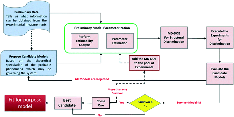
Fig. 1 presents the kinetic model (structure) identification framework, which includes all the steps starting from proposing the candidate models to arriving at the final fit for purpose model. The steps can be described as follows:1) Preliminary data: Experiments in the early development phases are rarely formally designed (e.g., DOE) but are executed simply with convenient conditions (i.e., temperature or initial concentrations) selected to get a broad understanding of the reaction's performance. This preliminary data is very limited in most cases because only a few grams of material are available for use at that time. One could argue that with all the advancements made in lab automation, there are smaller scale instruments and high throughput screening devices17 that can be used to generate sufficient data even from few grams. However, these technologies may not be always accessible for every project due to cost, resourcing, and scheduling.
2) Propose candidate models: Based on a theoretical understanding of the chemistry and the available data, process chemists/scientists propose a set of potential reaction pathways and the associated kinetic rate expressions for each of these proposed schemes. These kinetic expressions are the candidate models.
3) Preliminary model parameterization: Since the preliminary data is lean, it may be difficult to estimate all the model parameters simultaneously. As reviewed by McLean and McAuley,18 estimability analysis can be applied to highly non-linear models to obtain the rank ordering of estimable parameters to help select which parameters to estimate for a given model with a given set of experimental measurements. The performance of parameter estimation algorithms can be greatly improved by fitting only the high ranked parameters (with high estimability) and fixing the low ranked parameters to reasonable values. While fitting only the estimable parameters results in biased fits that are certainly not unique, it allows for easier convergence of the fitting algorithm and facilitates rapid model development, as the aim here is to quickly build a fit for purpose model for the early process development stages. The result of this workflow is a model that gives reasonable visual agreement to the available data; a formal lack of fit test would be inappropriate given the test assumptions and the biased parameter estimates.
4) Model-discrimination-design of experiment (MD-DOE): In this step, optimization approach is used to design experiment(s) that maximize the difference in predictions of the candidate models and therefore contains the information required to select the best model. An important activity in this step is to identify the response (manipulated) variables and determine which of these can be measured. Only those response variables that can be measured using the current experimental setup can be included in the DOE. Moreover, the measurement uncertainty will play an important role in determining the ability to discriminate between the candidate models. For example, if the measurement uncertainty is higher than the difference in prediction by the models then they can't be discriminated. The discriminatory experiment(s) will help select the most representative model structure within the region of interest. The formulation of the optimization problem is detailed later.
If none of the proposed models can satisfy the discriminatory experiment, then new candidate models should be proposed and steps 2–4 repeated.
5) Execute the experiments and evaluate the candidate models: Following execution of the MD-DOE, compare the experimental observation with the predictions by each candidate model. The candidate model with the closest prediction is the best model (survivor). Since the state of the model is still premature at this point, an accurate quantitative agreement shouldn't be expected. If there is more than one survivor, then the MD-DOE can be added to the pool of experiments and the whole exercise of model parameterization followed by model discrimination among the survivors (steps 3–5) can be repeated until one survivor is left. If it is impossible to discriminate between the candidates after a few iterations, then careful review of the models should help determine if a new intermediate concentration or other response should be quantified to help improve the MD-DOE. If there is no practical way to augment the dataset with discriminating information, then the modeler can choose one model to proceed with, as they are equivalent. The outcome of this exercise is a simple fit for purpose model.
2.1. Parameter estimation with Estimability analysis
For each candidate model, the estimability analysis is completed as follows:1) Define a set of initial guesses for the parameters. As a starting point, the initial guesses were obtained from chemical intuition and other related reactions. McLean and McAuley18 point out that the rank order of the parameters may change with change in the initial parameter values for a given set of experiments. Therefore, in case of any discrepancies, they advise to repeat the estimability analysis with a different set of initial guesses and check the reliability of the parameter ranking.
2) Identify the response variables that can be measured and obtain the sensitivity matrix.18 A summary of the calculation is provided in section S1 of the ESI.†
3) Apply a deflation algorithm to rank the parameters from the most to least estimable. The input to this algorithm is the scaled sensitivity matrix.16
4) The next step is to select the subsets of parameters that should be estimated or fixed so that the objective of the parameter estimation algorithm improves. Ranking the parameters is easy, however determining which parameters to estimate/fix is a difficult problem to solve. Researchers have tackled this problem in different ways as reviewed by Wu et al.16 In this work, we followed a similar methodology as Littlejohns et al.19,20 where we decided the number of parameters to be fixed based on the improvement observed in the objective function of the parameter estimation algorithm. We followed a brute-force method by fixing the parameters one by one starting with the lowest ranked parameter and moving up if a significant improvement in the objective function was observed. We stopped at a point where there was no further improvement in the objective function. While this process is tedious, it is easily implemented and for models of moderate size can be managed with some careful bookkeeping. A motivated practitioner could very easily script this process.
2.2. Model discrimination
The model discrimination was performed by executing a dynamic optimization of the non-linear problem as shown in eqn (1). Our discrimination criterion does not consider the model prediction uncertainty, since with a new API in the early phase of development there's not enough data/information available to understand it completely. Therefore, instead of making complex assumptions about the model prediction uncertainty, we are looking for gross differences in the model output, such that the simple criterion of finding the largest difference will find an experiment with a high likelihood of discriminating between the models. | (1) |
The steps of the model discrimination can be summarized as follows:
1) Use optimization techniques to solve eqn (1) and determine the experimental conditions, which will give the maximum difference between the predictions for the response variables by the candidate models.
2) Execute the MD-DOE.
3) Compare the model predictions with the actual experimental results.
4) The candidate models that cannot fit the discriminatory experiment are rejected.
3. Case study: identifying the best kinetic model structure from the proposed mechanisms of N-methylation of a compound
The methylation of heteroatom-containing molecules is an essential reaction in the preparation of countless bioactive compounds.21 The use of DMC (dimethyl carbonate) as a methylating agent has become increasingly popular as it offers a safer and eco-friendly alternative to toxic and unsafe reagents such as methyl halides and dimethyl sulfate.22One of the earlier limitations for the widespread use of DMC as the methyl source was that high temperatures and long reaction times were often required. However, in 2001, Shieh et al. reported that DBU (1,8-diazabicyclo[5.4.0]undec-7-ene) was an effective catalyst that enabled the O- and N-methylation of phenols, indoles and benzimidazoles under milder conditions.23 Shortly after, Shieh et al. expanded this chemistry to the methylation of benzoic acids and conducted a mechanistic investigation demonstrating that the DBU-catalyzed O-methylation of benzoic acids by DMC followed a mechanism that involved a DBU methyl carbamate 1 as the active methylating species, and not alternatives such as 2 (Fig. 2a).24 However, very recent findings indicate that any intermediates 1–4 could be plausible for the N-methylation and N-methoxycarbonylation of indoles (Fig. 2b).25,26
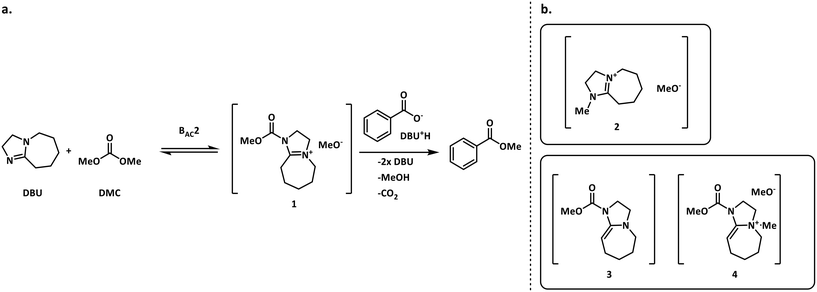 | ||
| Fig. 2 a. Shieh's mechanism for the DBU-catalyzed O-methylation of benzoic acid using DMC.24 b. Other possible reactive species in the N-methylation of indoles.25,26 | ||
Given that multiple mechanisms have been proposed and evidence supporting one or another has been brought forth, our own experience with a DMC-based and DBU-catalyzed N-methylation of an API intermediate compound would provide an ideal case study to evaluate our kinetic model identification framework elaborated in section 2.
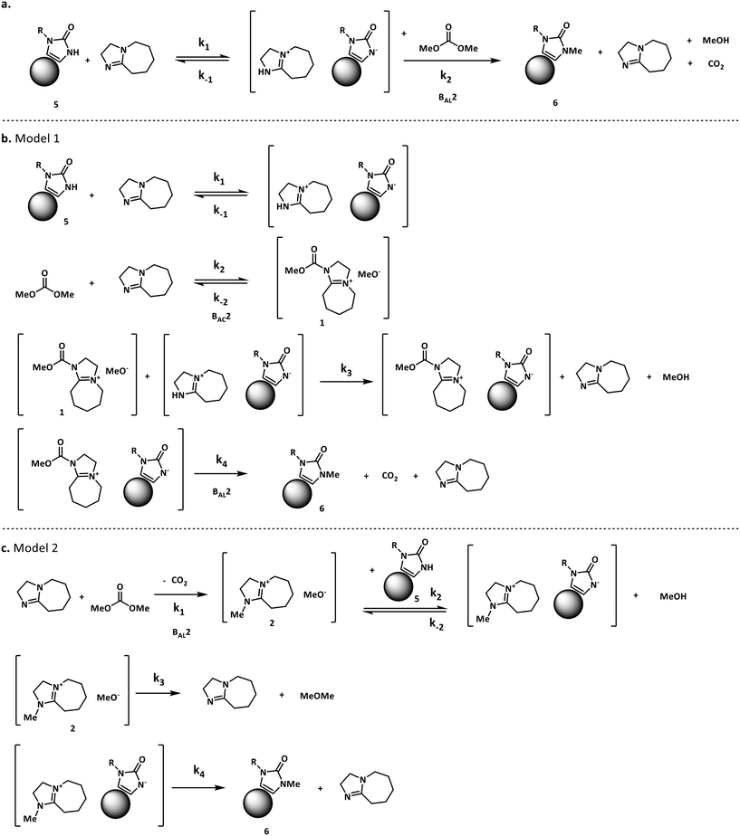
For our case study, three possible mechanisms for the conversion of compound 5 (starting material) into compound 6 (product) were considered and are shown in Fig. 3. Major portions of the molecule are undisclosed to protect intellectual property, however the relevant functional groups have been shown. In short, the three mechanisms explored here involve a) the direct alkylation of the starting material by DMC, b) the intermediacy of N-methoxycarbonylated DBU species (compound 1) and c) the presence of N-methylated DBU species (compound 2) as key to the kinetics of the reaction. Even though other variations to the three pathways depicted in Fig. 3 are possible, but were not comprehensively explored in this work since our objective is not to screen mechanisms, but to arrive at a suitable kinetic model structure that is predictive within our process space of interest. Moreover, in accordance with the work by Vendramini et al., that discredits species 3 and 4 as responsible for the N-methylation of indoles,25 other pathways including these species were not considered.
Fig. 3 depicts the first mechanism (a), where 5 is reversibly deprotonated by DBU, followed by a direct N-methylation with DMC by a BAL2 mechanism to afford compound 6 along with concomitant release of methanol and CO2. This mechanism as formulated is catalytic in DBU and could not explain the DBU consumption observed in the preliminary data, so it was removed from further consideration. The model fit results for this candidate are provided in Fig. A1 (section S2) in the ESI.†
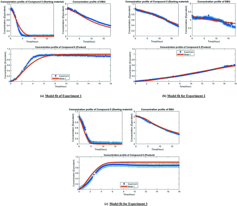
A mechanistic alternative is shown in Fig. 3 mechanism (b). The same acid–base equilibrium exists between 5 and DBU. However, in this case, DBU is proposed to react with DMC to generate the methylcarbamate ion pair 1 by a BAC2 mechanism. The methoxide component of this ion pair then reacts with the DBU conjugate acid to form a new ion pair composed of deprotonated 5 and the positively charged carbamate. This intermediate would then undergo N-methylation by a BAL2 mechanism to form the desired compound 6, release CO2 and regenerate DBU. The kinetic expression developed from this mechanism is the first candidate (model 1).
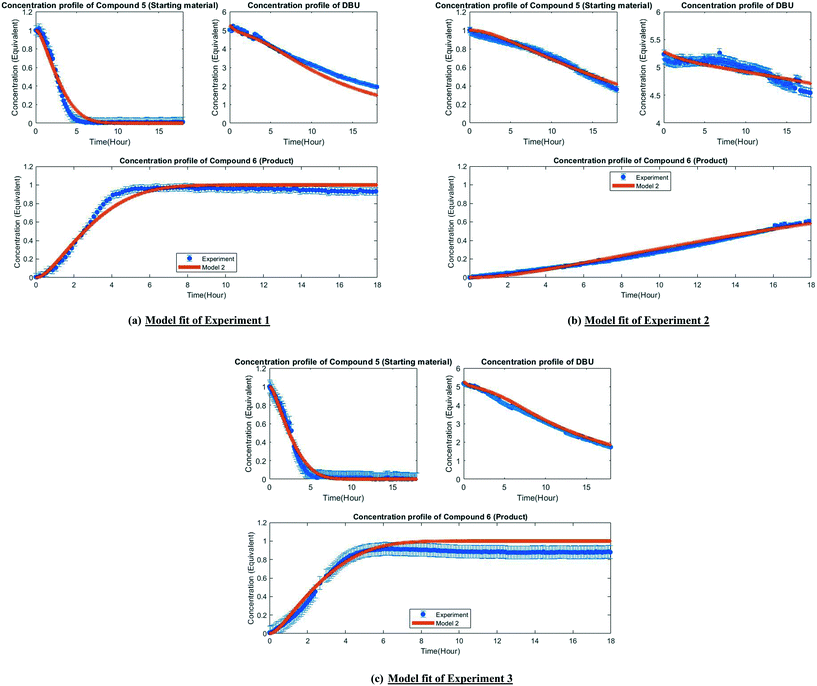
A third mechanistic hypothesis is presented in Fig. 3 mechanism (c). A different reaction between DBU and DMC is proposed, where CO2 release drives the formation of a N-methylated DBU/methoxide ion pair 2 by a BAL2 pathway. This ion pair could then react in two modes: first to deprotonate 5 and generate methanol and an ionic pair which would then undergo N-methylation to generate the desired compound 6 and release DBU. Alternatively, ion pair 2 could also undergo methoxide O-methylation to form dimethyl ether and DBU. The kinetic expression developed from this mechanism is the second candidate (model 2).
3.1. Experimental protocol
During the initial assessment, the available starting material was enough for conducting three controlled experiments at lab scale. The reactions were carried out in a batch mode under isothermal conditions. The molar fractions of the species have been monitored with flow NMR.27Analytical methods for measuring the concentration of compounds 5, 6 and DBU were developed. The concentrations of these three compounds will be referred to as the response or measured variables. Only these three compounds were profiled during the reactions. The control variables (or experiment settings) are the reaction temperature, and initial charge of the reactants. For simplicity, the initial volume of the reaction was assumed as: initial volume of reaction = initial volume of compound 5 charged + initial volume of DBU charged + initial volume of DMC charged.
| Compound 5 (initial mass) (mg) | DBU (initial volume) (μL) | DMC (initial volume) (μL) | Temperature (°C) | Initial volume of reaction (mL) | |
|---|---|---|---|---|---|
| Experiment 1 | 36 (1 equivalent) | 85 (5.3 equivalent) | 750 (83 equivalent) | 75 | 0.87 |
| Experiment 2 | 72 (1 equivalent) | 170 (5.3 equivalent) | 760 (42 equivalent) | 55 | 1.002 |
| Experiment 3 | 72 (1 equivalent) | 170 (5.3 equivalent) | 760 (42 equivalent) | 75 | 1.002 |
| MD-DOE | 64 (1 equivalent) | 24.9 (0.9 equivalent) | 9160 (572 equivalent) | 90 | 9.25 |
3.2. Model equations
 | (2) |
 | (3) |
 | (4) |
The rate constants: k1, k−1, k2, k−2, k3 and k4 in model 1, and k1, k2, k−2, k3 and k4 in model 2 were expressed as a function of temperature using the Arrhenius equation.
The unknown model parameters of model 1 are:
Frequency factor: A1, A−1, A2, A−2, A3 and A4.
Activation energy: E1, E−1, E2, E−2, E3 and E4.
The unknown model parameters of model 2 are:
Frequency factor: A1, A2, A−2, A3 and A4.
Activation energy: E1, E2, E−2, E3 and E4.
The candidate models were coded in gPROMS Formulated Product® (gFP®, Siemens Process Systems Engineering, London, UK) version 1.4.1. In some cases, estimating the frequency factor (A) directly may result in numerical instabilities. However, in our case this wasn't observed. gFP® has robust and powerful numerical solvers based off a variable step integration methodology that allows it to handle numerical stabilities very well. It can efficiently handle a complex model consisting of a large number of equations. This is a licensed and proprietary software developed by Siemens Process Systems Engineering, so more information is available in their documentation that comes with the software, but some basic information is available on their webpage.28
Note that the user may need to use an alternate formulation of the Arrhenius equation, e.g., a reference rate (kref) and temperature (Tref) as given by  in order to avoid any potential numerical instabilities depending on the platform they are using.
The purpose of this manuscript is to present the workflow on developing fit for purpose kinetic models during early phase pharmaceutical drug development with limited prior data and provisions to run experiments. Although the authors have implemented this workflow in gFP®, the users are free to use any platform/software of their choice.
3.3. Preliminary parameter estimation with estimability analysis
Several parameters (12 for model 1 and 10 for model 2) need to be estimated from only three experiments reported in Table 1 and only three measured responses (concentration of compound 5, DBU and compound 6). The parameter estimability code was written in MATLAB® 2019a (Mathworks, MA, USA). The parameter estimation was performed by using the built-in algorithm within gFP® version 1.4.1 that minimizes a modified form of the likelihood function.| Rank | Model 1 | Model 2 |
|---|---|---|
| 1 | E 2 | E 1 |
| 2 | E 1 | E 3 |
| 3 | E −2 | E 2 |
| 4 | E 4 | E 4 |
| 5 | E −1 | A 1 |
| 6 | E 3 | E −2 |
| 7 | A 2 | A 3 |
| 8 | A 1 | A 2 |
| 9 | A −2 | A 4 |
| 10 | A −1 | A −2 |
| 11 | A 3 | — |
| 12 | A 4 | — |
3.4. Model discrimination
In this section, the mathematical formulation of the optimization problem for model discrimination has been presented followed by a detailed description of the MD-DOE. | (5) |
| Temperature (T): TL ≤ T ≤ TU |
| Initial charge of Compound 5 (Cocpd5): CoLcpd5 ≤ Cocpd5 ≤ CoUcpd5 |
| Initial charge of DBU (CoDBU): CoLDBU ≤ CoDBU ≤ CoUDBU |
| Initial volume of reaction (VoR): VoLR ≤ VoR ≤ VoUR |
3.5. Experimental evaluation of MD-DOE and comparison with model predictions
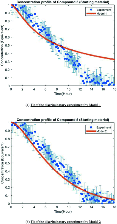
The MD-DOE supplies new information that can be used to improve the parameter estimates and model fit. Therefore, the estimability analysis was repeated after incorporating the MD-DOE along with the preliminary experiments. There was no significant change in the parameter ranking. The frequency factors continued to be ranked lower than the activation energies in the case of model 1. In the case of model 2, the parameters A2 and A3 inverted, but the remaining parameter ranks were as listed in Table 2. The parameter estimation was re-executed for both models with the MD-DOE added to the data pool. Fig. 6a and b illustrate the fit of the concentration profile of compound 5 obtained from the discriminatory experiment by model 1 and 2 respectively. Model 1 approaches an equilibrium at nearly 70% conversion, which is inconsistent with the experimental data. No improvement in the fit of model 1 was achieved even after incorporating estimability. Table A3 provided in the ESI† lists the final parameter values of model 1 after this exercise. The standard errors of the parameter estimates were small relative to the estimated parameter values. However, the model does not capture the reality observed in the MD-DOE experiment and can therefore be excluded on the grounds that the structure of the model equations is inconsistent with the data.Model 2 goes to completion and is consistent with the experimental data. Model 2 is therefore deemed the sole survivor model and is clearly applicable within a wider range of experimental conditions. Table 3 below presents the final parameter estimates of model 2. Parameters A2, A−2, A3 and A4 were fixed since these were low ranked parameters. As seen from the table, the standard errors of E−2 and E3 are very high, which means that these estimates can be improved further. The initial guesses, and the lower and upper bounds were also varied with no change in the results. To further improve the parameter estimates (i.e. reduce the standard errors of the parameters) one must add more diverse experiments to the data using methods described in the literature: Schwaab et al.,29 Shahmohammadi and McAuley,30 Quaglio et al.31 or Franceschini and Macchietto.32
| Model parameter | Final value | Initial guess | Search lower bound | Search upper bound | Standard error |
|---|---|---|---|---|---|
| A 1 | 0.041 × 10⁷ | 1.386 × 10⁷ | 0.01 × 10⁷ | 2 × 10⁷ | 0.021 × 10⁷ |
| A 2 (fixed) | 1 × 10¹² | 1 × 10¹² | 1 × 10¹² | 1 × 10¹² | |
| A −2 (fixed) | 4.674 × 10⁵ | 4.674 × 10⁵ | 4.674 × 10⁵ | 4.674 × 10⁵ | |
| A 3 (fixed) | 3.611 × 10⁵ | 3.611 × 10⁵ | 3.611 × 10⁵ | 3.611 × 10⁵ | |
| A 4 (fixed) | 3.019 × 10⁷ | 3.019 × 10⁷ | 3.019 × 10⁷ | 3.019 × 10⁷ | |
| E 1 | 74.776 × 10³ | 84.986 × 10³ | 1 × 10³ | 1000 × 103 | 1.493 × 10³ |
| E 2 | 99.679 × 10³ | 87.879 × 10³ | 1 × 10³ | 1000 × 103 | 0.115 × 10³ |
| E −2 | 78.772 × 10³ | 99.997 × 10³ | 1 × 10³ | 100 × 103 | 1.837 × 10¹² |
| E 3 | 12.146 × 10³ | 16 × 103 | 10 × 103 | 600 × 103 | 2.450 × 10⁸ |
| E 4 | 86.574 × 10³ | 86.908 × 10³ | 85 × 103 | 1000 × 103 | 0.485 × 10³ |
While beyond our present scope, we point out that improving parameter precision can be a very time consuming and costly endeavor and the decision to invest in that activity should depend on the model's purpose. For example, if the model is to be used as a part of the process control strategy to be filed as regulatory commitment, then precise model predictions are necessary that may require precise parameter estimates. However, if the model is used for providing guidance for process development and scaleup, the prediction accuracy from an early model may be sufficient with the expectation that further experiments will inform and confirm the process. In this work, model 2 was used in the later context to generate a process map to identify a suitable operational space. As an example of further application of the model, this process map is provided in Fig. A2 (section S6) in the ESI.†
4. Conclusion
Efficient use of available data and design of the next experiment to advance early understanding is a common industrial problem. As we have demonstrated with this case study, the procedure to design experiments to obtain a fit for purpose model in early process engineering can be readily implemented with standard software available to computational scientists and engineers and executed on standard issue hardware. The key aspect of the framework is application of estimability analysis to ensure that well posed parameter estimation problems are solved for the candidate models to allow for predictions that are acceptable for the purpose of designing discrimination experiments and guiding further experiments while the reaction is explored. In this case study, we have illustrated that three mechanisms proposed from chemical intuition for an N-methylation reaction can be reduced to a single model in a single cycle. This very real example showcases how adding modeling tools results in enhanced understanding even with very little available data. The framework discussed here can be easily extended into other unit operations where model discrimination or parameter estimation has proved intractable due to insufficient experiments.As a future endeavor, the authors would consider developing an open source generic framework to put the engineering tools as discussed in this work in the hands of other scientists (e.g., chemists) who play a key role in API process development. It is important that there is a smooth exchange of information between the engineering and other scientific communities. With the differences in general training and curricula among these respective communities there is a need to find an easy way to do so.
Author contributions
Maitraye Sen: conceptualization, data curation, formal analysis, investigation, methodology, software, visualization, writing (original draft), writing (review & editing). Alonso J. Arguelles: data curation, investigation, validation, writing (original draft), writing (review & editing). Stephen D. Stamatis: conceptualization, methodology, validation, writing (original draft), writing (review & editing). Salvador García-Muñoz: conceptualization, methodology, validation, project administration, supervision, writing (review & editing). Stanley Kolis: conceptualization, methodology, validation, project administration, supervision, writing (review & editing).Conflicts of interest
The authors have no conflicts of interest to disclose.Acknowledgements
The authors would like to acknowledge Carla Vanesa Luciani and Jonas Y. Buser for their help in running the NMR experiments.References
- P. M. Reilly and G. E. Blau, The use of statistical methods to build mathematical models of chemical reacting systems, Can. J. Chem. Eng., 1974, 52, 289–299 CrossRef.
- G. Box and W. Hill, Discrmination Among Mechanistic Models, Technometrics, 1967, 9, 57–71 CrossRef.
- B. Shields, J. Stevens, J. Li, M. Parasram, F. Damani, J. Alvarado, J. Janey, R. Adams and A. Doyle, Bayesian reaction optimization as a tool for chemical synthesis, Nature, 2021, 590, 89–96 CrossRef CAS PubMed.
- S.-H. Hsu, S. D. Stamatis, J. M. Caruthers, W. N. Delgass and V. Venkatasubramanian, Bayesian Framework for Building Kinetic Models of Catalytic Systems, Ind. Eng. Chem. Res., 2009, 48, 4768–4790 CrossRef CAS.
- Stan Development Team, Stan Modeling Language Users Guide and Reference Manual, Version 2.27, https://mc-stan.org, Accessed 9th September 2021 Search PubMed.
- F. Galvanin, E. Cao, N. Al-Rifai, A. Gavriilidis and V. Dua, A joint model-based experimental design approach for the identification of kinetic models in continuous flow laboratory reactors, Comput. Chem. Eng., 2016, 95, 202–215 CrossRef CAS.
- C. A. Hone, A. Boyd, A. O’Kearney-McMullan, R. A. Bourne and F. L. Muller, Definitive screening designs for multistep kinetic models in flow, React. Chem. Eng., 2019, 4, 1565–1570 RSC.
- S. Olofsson, L. Hebing, S. Niedenfuhr, M. P. Deisenroth and R. Misener, GPdoemd: A Python package for design of experiments for model discrimination, Comput. Chem. Eng., 2019, 9, 54–70 CrossRef.
- L. Violet, K. Loubiere, A. Rabion, R. Samuel, S. Hattou, M. Cabassud and L. Prat, Stoichio-kinetic model discrimination and parameter identification in continuous microreactors, Chem. Eng. Res. Des., 2016, 114, 39–51 CrossRef CAS.
- S. D. Schaber, S. C. Born, K. F. Jensen and P. I. Barton, Design, Execution, and Analysis of Time-Varying Experiments for Model Discrimination and Parameter Estimation in Microreactors, Org. Process Res. Dev., 2014, 18, 1461–1467 CrossRef CAS.
- M. Quaglio, L. Roberts, M. S. B. Jaapar, E. S. Fraga, V. Dua and F. Galvanin, An artificial neural network approach to recognise kinetic models from experimental data, Comput. Chem. Eng., 2020, 135, 106759 CrossRef CAS.
- L. X. Yu, G. Amidon, S. W. Hoag, J. Polli, G. Raju and J. Woodcock, Understanding Pharmaceutical Quality by Design, AAPS J., 2014, 16, 771–783 CrossRef CAS PubMed.
- L. Xu and F. X. X. Zhu, A new way to develop reaction network automatically via DFT-based adaptive kinetic Monte Carlo, Chem. Eng. Sci., 2020, 224, 115746 CrossRef CAS.
- Y. Wang and S. M. Huang, Commentary on Fit-For-Purpose Models for Regulatory Applications, J. Pharm. Sci., 2019, 108, 18–20 CrossRef CAS PubMed.
- L. Wright and T. Esward, Fit for purpose models for metrology: a model selection methodology, J. Phys.: Conf. Ser., 2013, 459, 012039 CrossRef.
- S. Wu, K. A. P. McLean, T. J. Harris and K. B. McAuley, Selection of Optimal Parameter Set Using Estimability Analysis and MSE-based Model-Selection Criterion, Int. J. Adv. Mechatron. Syst., 2011, 3, 188–197 CrossRef.
- A. Carnero, High Throughput Screening in drug discovery, Clin. Transl. Oncol., 2006, 8, 482–490 CrossRef CAS PubMed.
- K. A. P. McLean and K. B. McAuley, Mathematical Modelling of Chemical Processes- Obtaining the Best Model Predictions and Parameter Estimates Using Identifiability and Estimability Procedures, Can. J. Chem. Eng., 2012, 90, 351–366 CrossRef CAS.
- J. Littlejohns, K. McAuley and A. Daugulis, Model for a solid-liquid airlift two-phase bioscrubber for the treatment of BTEX, J. Chem. Technol. Biotechnol., 2010, 85, 173–184 CAS.
- J. Littlejohns, K. McAuley and A. Daugulis, Model for a solid-liquid stirred tank two-phase partitioning bioscrubber for the treatment of BTEX, J. Hazard. Mater., 2010, 175, 872–882 CrossRef CAS PubMed.
- E. J. Barreiro, A. E. Kummerle and C. A. M. Fraga, The Methylation Effect in Medicinal Chemistry, Chem. Rev., 2011, 111, 5215–5246 CrossRef CAS PubMed.
- P. Tundo and M. Selva, The Chemistry of Dimethyl Carbonate, Acc. Chem. Res., 2002, 35, 706–716 CrossRef CAS PubMed.
- W.-C. Shieh, S. Dell and O. Repic, 1, 8-Diazabicyclo [5.4. 0] undec-7-ene (DBU) and microwave-accelerated green chemistry in methylation of phenols, indoles, and benzimidazoles with dimethyl carbonate, Org. Lett., 2001, 3, 4279–4281 CrossRef CAS PubMed.
- W.-C. Shieh, S. Dell and O. Repic, Nucleophilic catalysis with 1, 8-diazabicyclo [5.4. 0] undec-7-ene (DBU) for the esterification of carboxylic acids with dimethyl carbonate, J. Org. Chem., 2002, 67, 2188–2191 CrossRef CAS PubMed.
- P. H. Vendramini, L. A. Zeoly, R. A. Cormanich, M. Buehl, M. N. Eberlin and B. R. Ferreira, Unveiling the mechanism of N-methylation of indole with dimethylcarbonate using either DABCO or DBU as catalyst, J. Mass Spectrom., 2021, 56(3), e4707 CrossRef CAS PubMed.
- M. Carafa, E. Mesto and E. Quaranta, DBU-Promoted Nucleophilic Activation of Carbonic Acid Diesters, Eur. J. Org. Chem., 2011, 2011, 2458–2465 CrossRef.
- J. Y. Buser and A. D. McFarland, Reaction Characterization by Flow NMR: Quantitation and Monitoring of Dissolved H2 via Flow NMR at High Pressure, Chem. Commun., 2014, 50, 4234–4237 RSC.
- Siemens, gPROMS formulatedProducts, https://www.psenterprise.com/products/gproms/formulatedproducts/solids/software-features, Accessed 18th August 2021.
- M. Schwaab, J. L. Monteiro and J. C. Pinto, Sequential experimental design for model discrimination: Taking into account the posterior covariance matrix of differences between model predictions, Chem. Eng. Sci., 2008, 63, 2408–2419 CrossRef CAS.
- A. Shahmohammadi and K. B. McAuley, Sequential model-based A- and V-optimal design of experiments for building fundamental models of pharmaceutical production processes, Comput. Chem. Eng., 2019, 129, 106504 CrossRef CAS.
- M. Quaglio, E. Fraga and F. Galvanin, Model-based design of experiments in the presence of structural model uncertainty: an extended information matrix approach, Chem. Eng. Res. Des., 2018, 136, 129–143 CrossRef CAS.
- G. Franceschini and S. Macchietto, Model-based design of experiments for parameter precision: State of the art, Chem. Eng. Sci., 2008, 63, 4846–4872 CrossRef CAS.
Footnote |
| † Electronic supplementary information (ESI) available. See DOI: 10.1039/d1re00222h |
| This journal is © The Royal Society of Chemistry 2021 |

