
 Open Access Article
 This Open Access Article is licensed under a
 Creative Commons Attribution 3.0 Unported Licence
A novel approach for kinetic measurements in exothermic fixed bed reactors: advancements in non-isothermal bed conditions demonstrated for methanol synthesis†
F.
Nestler
 *a,
V. P.
Müller
a,
M.
Ouda
a,
M. J.
Hadrich
a,
A.
Schaadt
a,
S.
Bajohr
b and
T.
Kolb
b
*a,
V. P.
Müller
a,
M.
Ouda
a,
M. J.
Hadrich
a,
A.
Schaadt
a,
S.
Bajohr
b and
T.
Kolb
b
aFraunhofer Institute for Solar Energy Systems ISE, Heidenhofstr. 2, 79110 Freiburg, Germany. E-mail: florian.nestler@ise.fraunhofer.de
bEngler-Bunte-Institute EBI, Engler-Bunte-Ring 2, 76161 Karlsruhe, Germany
First published on 21st April 2021
Abstract
Kinetic modelling of methanol synthesis remains one key challenge for the implementation of power-to-methanol technologies based on CO2-rich gas streams and sustainably produced H2. Within this work, a novel approach for kinetic model validation and parameter estimation using an experimental miniplant setup with polytropic bed conditions is presented. The miniplant setup features a highly resolved fibre optic temperature measurement combined with FTIR product composition analysis. Comparison of the experimental temperature and concentration data to a simulation model applying literature kinetic models, confirmed the necessity of axial experimental data to deliver an appropriate kinetic description of the methanol synthesis reaction network. A refitting of the literature kinetic models was performed in order to enhance their capability to account for the catalytic behaviour of a modern commercial catalyst. Besides the traditional measurement of the outlet concentration, it was shown that the temperature profile as a direct consequence of exothermic reactions in polytropic miniplant setups can be used to derive an improved kinetic description if appropriate models for heat transfer and diffusion are provided. Finally, the behaviour of the proposed new kinetic model is discussed on the industrial scale by means of a sensitivity analysis emphasizing the applicability of the presented novel approach for the scale-up from miniplant to industrial scale.
Introduction
The rising demand for energy carriers and base chemicals produced from sustainably generated hydrogen (H2), e.g. by water electrolysis, in the context of power-to-X (PtX) processes recently created vast research activity with the aim of making alternative synthesis routes competitive to their fossil counterpart.1 Among the most promising PtX products, ammonia (NH3), synthetic natural gas (SNG) and methanol (MeOH) are discussed.2 In this context, methanol is very likely to play a key role due to its capability as carbon dioxide (CO2)-sink when combined with industrial processes, as cement or steel production. Moreover, methanol has the advantage of an already existing trade infrastructure and is a key molecule for production of high value derivatives such as polymers, fuels and olefins. With an annual production capacity of approximately 100 Mt methanol is already today an important platform molecule for the chemical industry and the energy sector.3Despite the fact of methanol synthesis being one of the oldest thermochemical high pressure processes, questions remain open on the adaption of the process from fossil-based synthesis gas (syngas) with high carbon monoxide (CO)-contents towards sustainable syngas with high CO2-contents.4,5 As both, electrolytically produced H2 from renewable energy and carbon oxide-rich gas obtained from the coupled industrial process are subjected to fluctuations,4 dynamic description of the methanol synthesis process and the synthesis reactor are imperative for the implementation of PtM processes.6–8 However, dynamic operation of the methanol synthesis reactor demands for a validated simulation including a highly reliable kinetic model. Therefore, an improved kinetic understanding of methanol synthesis is one key issue for the implementation of PtM technology on the industrial scale.9
In general, methanol synthesis carried out on commercial Cu/Zn/Al2O3-catalysts can be expressed via the following exothermic equilibrium limited reactions:10
| CO2(g) + 3H2(g) ⇄ CH3OH(g) + H2O(g) ΔH0R = −50 kJ mol−1 | (1) |
| CO(g) + H2O(g) ⇄ CO2(g) + H2(g) ΔH0R = −41 kJ mol−1 | (2) |
| CO(g) + 2H2(g) ⇄ CH3OH(g) ΔH0R = −91 kJ mol−1 | (3) |
For reactor design, the temperature and the axial position of the hot spot, i.e. the point with the highest temperature inside the reactor, represent important key parameters.21–26 In one of our previous studies we demonstrated significant discrepancies regarding the simulative description of the hot spot depending on the choice of the kinetic model.27 Consequently, substantial uncertainties in reactor and process design are obtained leading towards oversizing of process equipment and application of too mild process conditions, e.g. low synthesis temperatures.22
Classic kinetic experimental setups are built with respect to minimal temperature gradients along the radial and axial coordinate of the fixed bed allowing a simple temperature measurement and straightforward validation of reaction kinetics.28–30 Besides pressure and temperature, key parameters in kinetic measurements in methanol synthesis usually address the variation of the carbon oxide ratio (COR), the stoichiometric number (SN) and the gas hourly space velocity (GHSV). The three parameters are formulated as follows:4
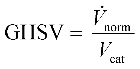 | (4) |
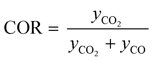 | (5) |
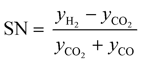 | (6) |
Due to the lack of experimental data, possible issues arise when the kinetic models derived in ideally isothermal fixed bed reactors are transferred to an industrial reactor featuring non-isothermal bed conditions. Differentially resolved kinetic data would be mandatory in order to deliver a local reaction rate along the axial reactor dimension in an industrial reactor with appropriate accuracy.27
This work introduces a novel approach applying a polytropic miniplant reactor scaled down from an industrial steam cooled multi-tubular reactor for the validation of kinetic models for exothermic fixed bed reactions. The validation relies on a highly resolved measurement of the axial temperature profile inside the reactor in addition to the product gas analysis. By gathering information on the axial temperature profile, the quantity of validation information can be increased significantly in comparison to traditional integral fixed bed measurements. Importantly, the transferability of the derived improved kinetic model on industrial scale will be demonstrated. Moreover, an optimization of the miniplant dimensions will be carried out in order to increase the similarities between industrial and miniplant reactor scale.
Methods
The validation approach presented within this work strongly relies on a detailed simulation model of the miniplant reactor. In order to discuss the derived kinetic model also on the industrial scale, ability of the simulation to adapt to this scale was of high importance for this work. Therefore, the implementation of the simulation platform used in this work will be described first. Subsequently, the scale-down and design of the experimental setup as well as the methodology for the kinetic parameter estimation will be presented. Finally, the methodology for the discussion of the derived kinetic model on the industrial scale will be explained.Simulation platform
In order to use a non-isothermal experimental setup for validation and parameter fitting of a kinetic model, a simulation platform for the description of the methanol synthesis reactor was developed. This platform can be described as a wrapper allowing the reactor simulation to be adaptable to different scales and geometries.The reactor model is based on sub-models describing heat transfer, powder kinetics and diffusion inside the reactor. As shown in Fig. 1, powder kinetics and diffusion model express the effective particle kinetics, which are then included into the numerical one-dimensional reactor model.
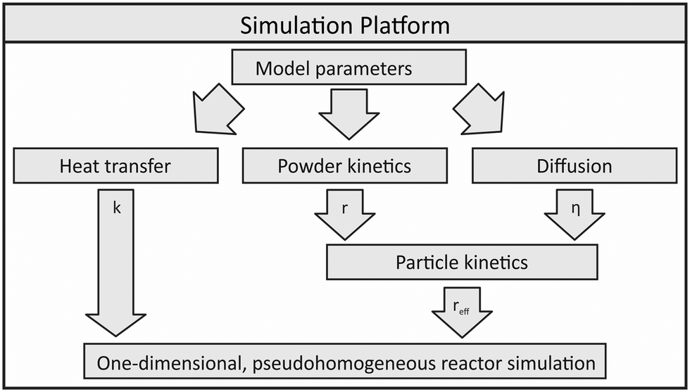 | ||
| Fig. 1 Simulation platform applied within this publication. | ||
 | (7) |
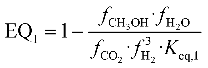
CO2-hydrogenation
 | (8) |
 | (9) |
 | (10) |
 | (11) |
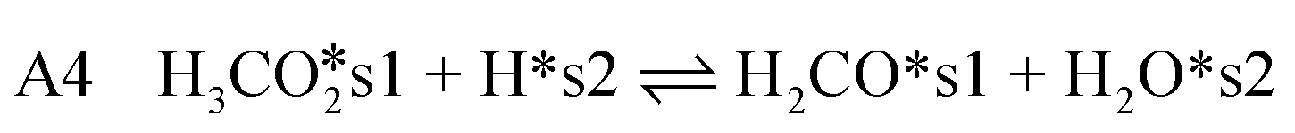
| A5 H2CO*s1 + H*s2 ⇌ H3CO*s1 + s2 | (12) |
| A6 H3CO*s1 + H*s2 ⇌ CH3OH + s1 + s2 | (13) |
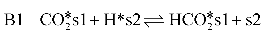
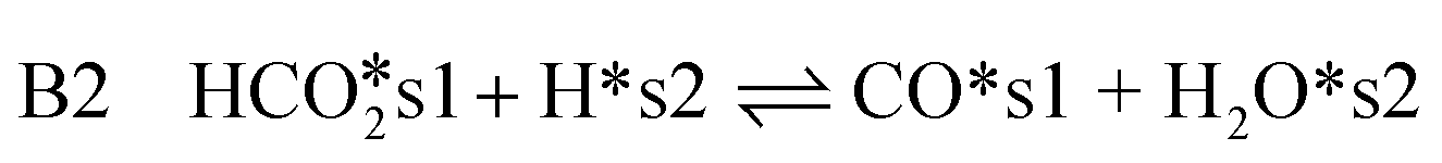
rWGS
 | (14) |
 | (15) |
 | (16) |
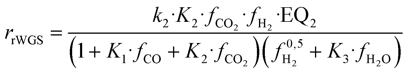 | (17) |
 | (18) |
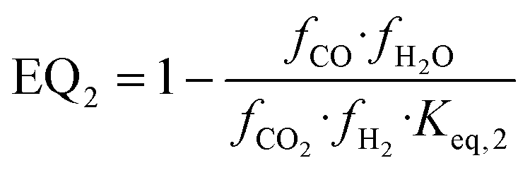 | (19) |
 | (20) |
 | (21) |
 and
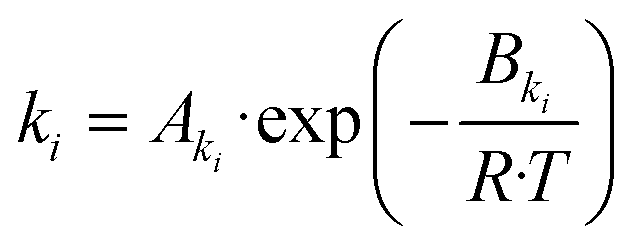
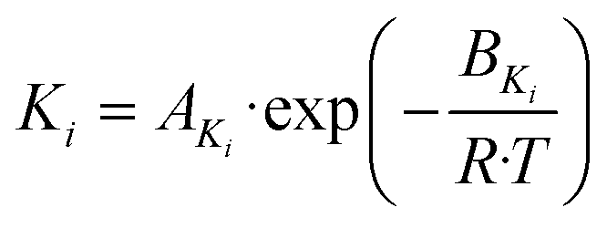
and  representing the pseudo equilibrium constant50 as well as
  and
and  as pseudo-first-order rate constant:52
 | (22) |
 | (23) |
| Parameter | Unit | Value |
|---|---|---|
| τ | — | 2.99 |
| ε p | — | 0.58 |
The efficiency factor of the reactions ηeff is calculated for both, water and methanol as follows:50,52
 | (24) |
 | (25) |
 | (26) |
 | (27) |
 | (28) |
![[V with combining dot above]](https://www.rsc.org/images/entities/i_char_0056_0307.gif) at rated pressure and temperature:
at rated pressure and temperature: | (29) |
| Parameter | Unit | Value |
|---|---|---|
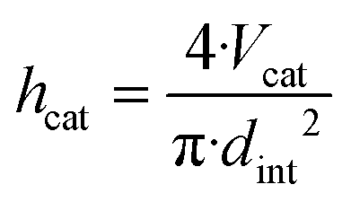
| d int | m | 3.8 × 10 −2 |
| h cat | m | 7.022 |
| d p | m | 5.4 × 10 −3 |
| ε bulk | — | 0.39 |
| ρ bulk | kg m−3 | 1132 |
Experimental
- The Bodenstein number with the axial dispersion coefficient calculated according to Kraume60
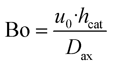 | (30) |
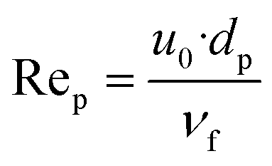
- The Reynolds particle number (see eqn (28))
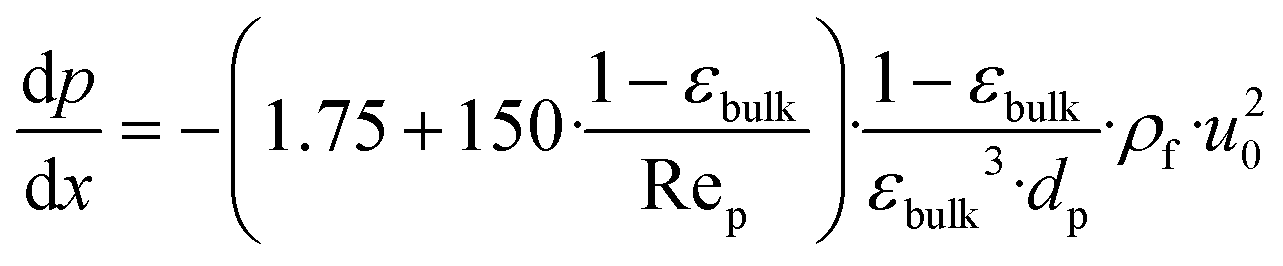
- The reactor-particle diameter ratio61
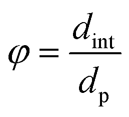 | (31) |
With regard to methanol synthesis as one of the oldest high pressure reactions, versatile research has been performed and rich knowledge on the modelling of heat transfer, kinetics and diffusion was published in the past decades.10,63 Therefore, a simulation-based approach was realised in our work in order to design an experimental miniplant setup with a high transferability of the experimental results towards industrial scale. As a key parameter, the GHSV was held equal for both industrial and miniplant reactor simulation in order to obtain similar residence times inside the reactor on both scales.
Based on this approach and infrastructural boundary conditions, the miniplant setup used within this work was designed and built. The following procedure was applied to design the reactor dimensions:
1.) Definition of the miniplant scale considering the lab infrastructure.
2.) Design of a cooling system for a comparable heat transfer in the miniplant related to the industrial scale.
3.) Optimization of the reactor dimensions by minimizing the difference between the simulated temperature profiles of the industrial reactor and the miniplant using the simulation platform.
In contrast to the industrial reactor implemented as multi tubular steam cooled reactor, the miniplant reactor consists of a double pipe arrangement with thermal oil circulated through the annular gap while the catalyst is placed inside the inner tube. The idea behind the thermal oil cooling of the miniplant was to counter-balance the higher cooling-area-to-catalyst-volume ratio of the miniplant in comparison to the industrial reactor. The overall objective of this advanced cooling concept was to achieve a temperature profile inside the miniplant reactor comparable to that of the industrial reactor.
In order to determine the reactor dimensions for a maximised comparability of the miniplant setup to the industrial scale, the diameter of the miniplant setup was varied with the catalyst bed length adjusted to the previously defined catalyst volume Vcat correspondingly:
 | (32) |
 | (33) |
By performing simulations for both, industrial and miniplant setup, the dimensions listed in Table 3 were iteratively defined.
The dimensionless index numbers defined previously are provided for both, industrial and miniplant setup in Table 4.
| Parameter | Unit | Industrial reactor55 | Miniplant reactor |
|---|---|---|---|
| Bo | — | 1014 | 900 |
| φ | — | 7.04 | 13 |
| Rep | — | 1185 | 36 |
Comparison of the dimensionless indices shows that both reactor scales satisfy the criterions for ideal plug flow,32i.e. Bo > 80, and non-laminar particle flow, i.e. Rep > 10. The difference of the Rep numbers between industrial and miniplant reactor due to the adjusted reactor and catalyst geometries was considered in the simulation of pressure loss as well as convective heat transfer inside the reactor. As the reactor-particle-ratio satisfies the criterion φ > 10 wall effects in the miniplant were neglected.28,32 However, in case of the industrial reactor φ was below this critical threshold. Measured data obtained from this reactor would be helpful to quantify possible deviations from the herein assumed ideal plug flow behaviour for the industrial reactor.
The inner diameter of 13 mm for the miniplant reactor was obtained by the simulation-based scale-down utilizing the kinetic model by Bussche-Froment15 at high CO2-contents. As the choice of the kinetic model was found to influence the optimal reactor dimensions significantly, optimised miniplant dimensions applying the kinetic model derived within this work will be presented at the end of this study. These were determined for a wide range of synthesis conditions covering two different pressure levels of 50 bar and 80 bar at GHSV = 9000 h−1. Feed gas composition was varied in the range 2.0 ≤ SN ≤ 8.0 and 0.5 ≤ COR ≤ 1.0.
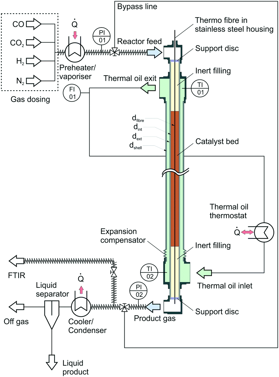 | ||
| Fig. 2 Simplified flow sheet of the experimental setup. | ||
The heat released by the reaction inside the inner tube was removed by thermal oil circulating along the annular gap in counter current flow. Volumetric flow rate of the oil was measured by a rotameter calibrated for the thermal oil used inside the cooling system (Fragoltherm X-400-A). Temperature of the thermal oil was controlled by a closed-cycle thermostat.
The reactor was filled with a commercial Cu-based catalyst provided by Clariant. The pelletised catalyst particles were ground and sieved to a particle size of dp = 1 mm to avoid wall effects inside the reactor. An inert bed of α-alumina supplied by Merck KGaA was placed above and below the catalyst bed. The fixed bed was held inside the reactor with a porous stainless steel support disc. Preliminary tests introducing syngas into the heated reactor filled with only the inert material confirmed the inert behaviour of the whole setup.
In order to gather axial information about the reaction kinetics, the reactor was equipped with a system for fibre optical temperature measurement. The measurement principle of this technology is based on axial variation of the refractive index along a glass fibre due to impurities or local defects.65 Application of Fourier transformation to a back-scattered light signal leads towards continuous information about (thermal) expansion of the fibre and thereby delivers a spatially resolved temperature information. The glass fibre was placed inside a 0.8 mm steel capillary; the optical signal was generated and processed by a Luna ODiSI 6102 unit. An axial resolution of Δx = 2.6 mm was selected for the measurement campaign leading to 431 measurement increments for temperature measurement (NT,inc) inside the catalyst bed with a length of 1.12 m. Calibration of the fibre was carried out by heating the thermal oil cycle to constant temperature levels between 50 °C and 265 °C. The oil inlet and outlet temperatures were measured by two Pt-100 temperature sensors at the oil inlet (TI02) and outlet (TI01); a heat loss resulting in a temperature decrease of approximately 1.5 K between thermal oil inlet and outlet was regarded by a linear temperature decrease along the reactor. The cooling temperature Tcool was adjusted to the reading of TI01. As a result of the calibration a polynomial of 3rd degree was determined for each increment along the fibre. Extrapolation of these polynomials was performed for temperatures exceeding 265 °C as the thermal oil did not allow for higher calibration temperatures due reasons of plant safety.
For analysis of the reaction products a MKS MultiGas™ 2030 on-line FTIR with an optical path length of 35 cm was used for quantitative product analysis. Since H2 as a homonuclear gas cannot be detected by FTIR, the molar fraction of this gas was determined by the component balance as follows:
 | (34) |
Besides the gas phase analysis, the main product stream was led through a cooler-condenser unit at an operating temperature of 10 °C to separate the liquid products from the gas phase for qualitative analysis of condensable trace compounds. Analysis of the liquid phase was carried out using NMR spectroscopy.
All real time information on sensor properties such as volumetric flow rates, inlet and outlet pressures, temperature profile as well as gas phase composition were logged with a sample rate of 1 Hz.
The variation ranges of the experimental parameters are provided in Table 5. All combinations of parameters listed were applied to the experimental setup at a cooling temperature of 240 °C.
| Parameter | Varied range |
|---|---|
| p | 50 bar; 65 bar; 80 bar |
| GHSV | 6000 h−1; 9000 h−1; 12![[thin space (1/6-em)]](https://www.rsc.org/images/entities/char_2009.gif) 000 h−1 000 h−1 |
| COR | 0.7; 0.8; 0.9; 0.95; 0.98 |
| SN | 2.0; 3.0; 4.0; 5.0; 6.0; 7.0; 8.0 |
To consider the effect of lower temperatures the parameter variation at 50 bar was also executed at a cooling temperature of 220 °C in a COR range between 0.7 and 0.95. Due to instability of some experimental points as a result of oscillations in CO2 dosing or hot spot temperatures expected to exceed the critical threshold of 280 °C, some of the data points could not be included into the validation resulting in an overall set of 324 data points (Ndata pt). To account for activity changes during the experimental campaign a benchmark measurement was repeatedly executed. The benchmark condition was defined at COR = 0.9, SN = 4.0, GHSV = 12000 h−1 and Tcool = 240 °C.
The experimental plan was executed in seven phases as follows:
1.) Ramp-up at benchmark conditions at 50 bar:
2.) p = 50 bar; Tcool = 240 °C; SN = 4.0; COR = 0.9; GHSV = 12000 h−1;
3.) Parameter variation at 50 bar and 240 °C:
4.) p = 50 bar; Tcool = 240 °C; 2.0 ≤ SN ≤ 8.0; 0.7 ≤ COR ≤ 0.95; 6000 h−1 ≤ GHSV ≤ 12000 h−1.
5.) Parameter variation at 65 bar and 240 °C:
6.) p = 65 bar; Tcool = 240 °C; 2.0 ≤ SN ≤ 8.0; 0.7 ≤ COR ≤ 0.95; 6000 h−1 ≤ GHSV ≤ 12000 h−1.
7.) Parameter variation at 80 bar and 240 °C:
8.) p = 80 bar; Tcool = 240 °C; 2.0 ≤ SN ≤ 8.0; 0.7 ≤ COR ≤ 0.95; 6000 h−1 ≤ GHSV ≤ 12000 h−1.
9.) Parameter variation at COR = 0.98 and 240 °C;
10.) 50 bar ≤ p ≤ 80 bar; Tcool = 240 °C; 2.0 ≤ SN ≤ 8.0; COR = 0.98; 6000 h−1 ≤ GHSV ≤ 12000 h−1.
11.) Parameter variation at 50 bar and 220 °C:
12.) p = 50 bar; Tcool = 220 °C; 2.0 ≤ SN ≤ 8.0; 0.7 ≤ COR ≤ 0.95; 6000 h−1 ≤ GHSV ≤ 12000 h−1.
13.) Benchmark at conditions of phase (1).
During phase 1.) the benchmark conditions were held constant for 56 h. In phase 5.) COR was held constant at 0.98 at the three pressure levels considered. This variation was not included into phases 2.) to 4.) as catalyst deactivation was expected during these experiments due to the high CO2 content. After the parameter variation was terminated, the benchmark point of phase 1.) was held constant for another 12 h.
Validation and parameter fitting
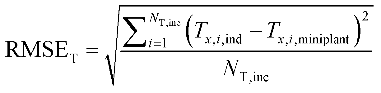
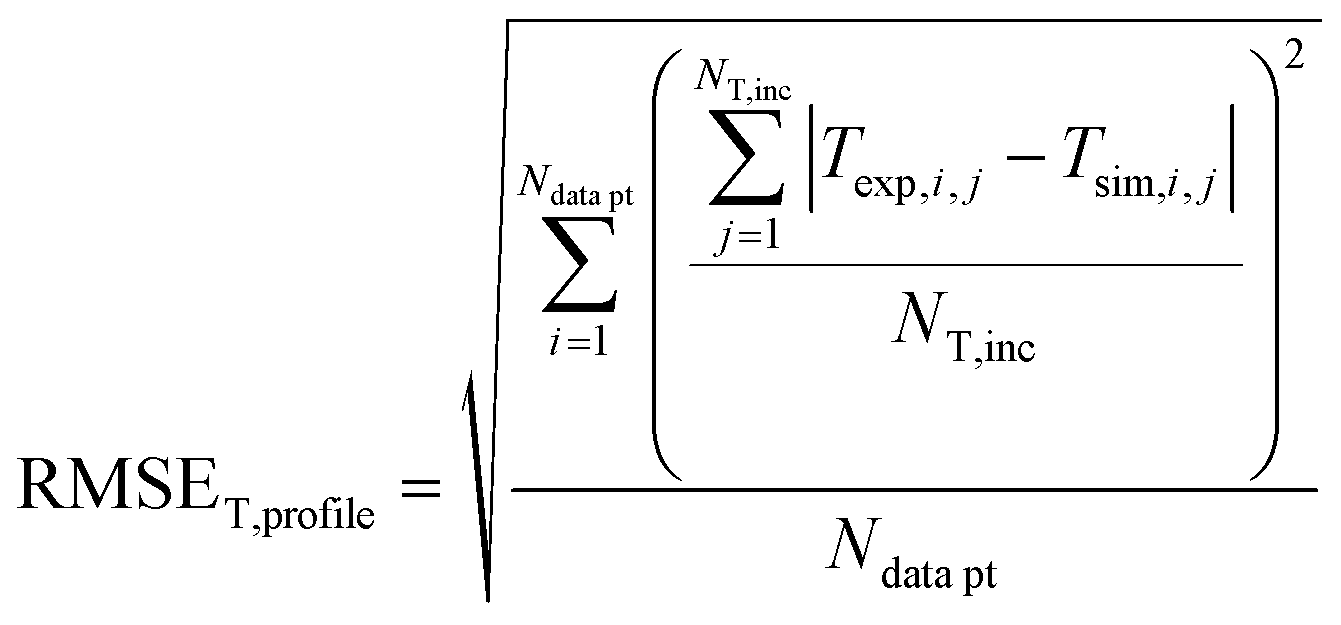
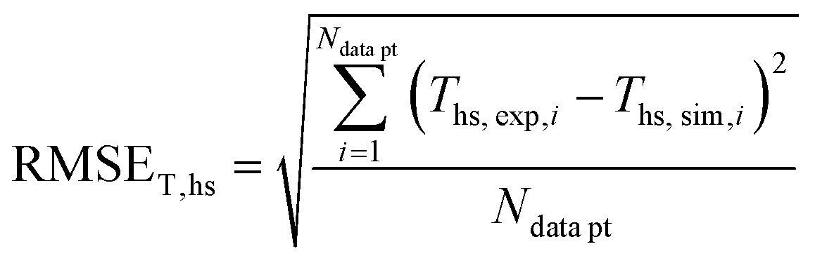
In order to validate the behaviour of literature kinetic models in comparison against the data acquired within this study and to optimise their behaviour by a parameter variation, information on gas phase composition and temperature profile for each working point were fed into a validation library. A reactor simulation was carried out for all documented working points to determine deviations between model and experiment.A multi-criterial optimization changing the parameters of the utilised kinetic models, i.e. kinetic constants and adsorption constants, was executed in order to minimise the deviation between the reactor simulation and the experimental data. The objective function f(x) for the parameter fitting was formulated as the sum of the weighted root mean square errors for temperature profile (RMSET,profile), for hot spot temperature (RMSET,hs) and gas phase composition at reactor outlet (RMSEy):
| f(x) = α·RMSET,profile + β·RMSET,hs + γ·RMSEy | (35) |
 | (36) |
 | (37) |
 | (38) |
f(x) was minimised by the fminsearch algorithm using MATLAB.64 Local minima were mitigated by restart of the algorithm, as the resulting expansion of the simplex around the local optimum proved to lead towards parameter combinations with an improved objective function. Application of global optimisers as the State Transition Algorithm published by Zhou et al.66 turned out to be too inefficient for the optimization problem in hand. Methodology of the parameter fitting applied within this study is depicted in Fig. 3.
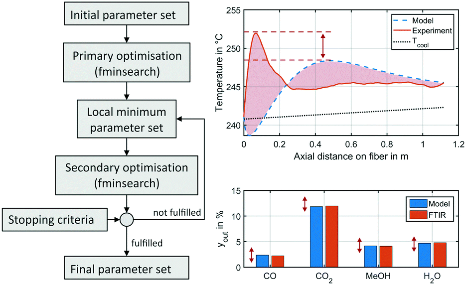 | ||
| Fig. 3 Illustration of parameter fitting applied in this study (left) and an exemplary working point a benchmark conditions at 50 bar showing the temperature profile (right, top) and gas phase molar fractions (right bottom) obtained from the experiment (solid, red) and the miniplant reactor simulation (dotted, blue) using the original kinetic model by Nestler;27 red arrows and area indicate errors minimised by the parameter fitting; the measured temperature profile is smoothened by the Savitzky–Golay filter.67 | ||
Due to slight heterogeneity in the distribution of catalyst particles along the fibre's shell, fluctuations in temperature measurement were identified along the axial reactor dimension. In order to simplify the process parameter estimation of the kinetic rate equations, temperature profiles of each data point were smoothened applying the Savitzky–Golay filter.67 This algorithm eliminates noise from a signal by application of fitted polynomials over a defined window of data points. A second-degree polynomial with a moving window of 40 elements was applied. A smoothened temperature profile at benchmark working conditions at 50 bar is shown in Fig. 3 on the right in comparison to the miniplant reactor simulation performed using the kinetic model of our previous study.27 Red areas and arrows indicate the errors minimised by the parameter fitting.
Discussion of the impact on industrial reactor design
In order to demonstrate the impact of the new kinetic model on the industrial scale reactor in comparison to our previously published model,27 a simulation study was performed analysing hot spot position and temperature as well as product composition, in an industrial reactor simulation at the three pressure levels 50 bar, 65 bar and 80 bar at GHSV = 6000 h−1. For the gas composition the range applied in the experimental campaign was considered (see Table 5). Inlet and cooling temperatures were set to 240 °C.Results and discussion
Experimental results
Experimental data obtained from the miniplant setup indicated strong sensitivities of hot spot temperature, product composition and space time yield (STY) towards pressure, stoichiometry and COR. However, the measurement campaign was overlaid by a continuous deactivation of the catalyst. In Fig. 4 STY is plotted over experimental time-on-stream (ToS) for the benchmark composition of SN = 4.0 and COR = 0.9 at the three pressure levels as well as the two cooling temperatures applied in this study. The graph indicates that STY stabilised during ramp up after approx. 50 h ToS. However, stronger deactivation of the catalyst was observed during the experimental plan at 80 bar (phase 4.)) and COR = 0.98 (phase 5.)). As both, the highest temperatures and the highest water contents were measured during these phases, based on these observations it can be concluded that the deactivation of the catalyst was mainly correlated to these two factors. This is in good agreement to the work of Fichtl et al. who considered hydrothermal degradation of the active sites as the main reason for catalyst deactivation in cleaned syngas.68 However, their group showed the necessity for longer experimental campaigns exceeding 1600 h ToS to obtain satisfactory information about deactivation kinetics. As this, though, was not in the scope of our study, the influence of catalyst deactivation was not yet included within our study consequently leading towards inaccuracies for the kinetic fitting. Future research is planned in our group to derive advanced axially resolved deactivation kinetics using the experimental setup described herein.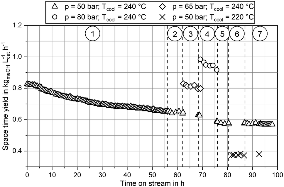 | ||
| Fig. 4 Trend of the space time yield over time-on-stream at benchmark conditions COR = 0.9; SN = 4.0; GHSV = 12000 h−1 at 50 bar, 65 bar and 80 bar at Tcool = 240 °C and Tcool = 220 °C. Sectors marked: 1.) ramp up, benchmark at 50 bar, 240 °C; 2.) experimental plan at 50 bar and 240 °C; 3.) experimental plan at 65 bar and 240 °C; 4.) experimental plan at 80 bar and 240 °C; 5.) variation of SN at COR = 0.98, 240 °C and 50 bar to 80 bar; 6.) experimental plan at 50 bar, 220 °C; 7.) benchmark at 50 bar, 240 °C. | ||
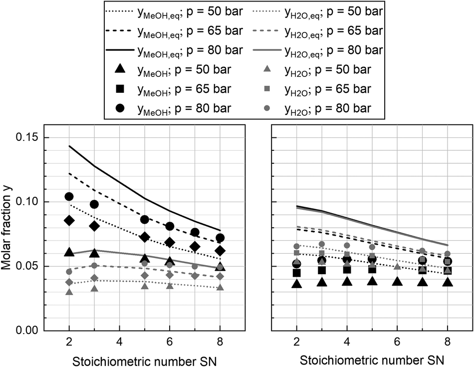
In Fig. 5 the molar fractions of water and methanol obtained from the experiments at GHSV = 12000 h−1 and a cooling temperature of 240 °C at the three pressure levels for COR = 0.7 (left) and COR = 0.95 (right) are depicted over SN. Thermodynamic equilibrium for the data points was calculated at reactor outlet temperature applying the equilibrium constants published by Graaf et al.44 As shown by the difference between equilibrium and measured molar fraction of methanol, all experiments at this GHSV were carried out inside the kinetic regime of the methanol reaction. However, water production did reach the thermodynamic equilibrium, probably due to higher reaction kinetics of rWGS. As expected considering Le Chatelier's principle, increased synthesis pressures led towards increased equilibrium molar fractions of methanol and water and consequently to higher reaction kinetics due to an enhanced driving force. The highest methanol molar fraction was obtained at COR = 0.7 and SN = 2.0. While at COR = 0.7 an increase of SN led towards a decrease of methanol molar fraction, the molar fraction of methanol was not sensitive to SN at COR = 0.95. This finding can be explained with the rate inhibiting effect of high water partial pressures that was already recorded in literature.11,69,70
 | ||
| Fig. 5 Equilibrium and measured molar fraction of methanol (black) and water (grey) at COR = 0.7 (left) and COR = 0.95 (right); equilibrium molar fractions at 50 bar (dotted), 65 bar (dashed) and 80 bar (solid); measured molar fractions of methanol and water at GHSV = 12000 h−1 at 50 bar (triangle), 65 bar (diamond) and 80 bar (circle). | ||
Besides product concentration, another indicator for the catalytic activity can be gathered from the temperature profile inside the reactor. In Fig. 6 the hot spot temperatures for the three pressure levels at GHSV = 12000 h−1 and COR = 0.7 and COR = 0.95 are plotted over SN. The graph indicates a strong correlation between COR and the achieved temperatures inside the reactor. While at COR = 0.7 a maximum hot spot temperature of 278 °C was reached (SN = 2.0; p = 80 bar), temperatures were on a significantly lower level at COR = 0.95 with a maximum hot spot temperature of 257 °C at SN = 5.0 and p = 80 bar. This can be explained as an increase of CO molar fraction in the feed gas decreases the amount of water produced and consequently increases the reaction rates for methanol synthesis. Due to the higher exothermic heat released inside the reactor (eqn (3)), heat removal requires a higher temperature difference between cooling fluid and catalyst, leading towards an increase of hot spot temperature. The hot spot position was measured between 0.1 m and 0.2 m downstream the start of the catalyst bed at COR = 0.7 and at 0.06 m at COR = 0.95, respectively. Due to heterogeneities of the particle distribution along the temperature sensor, a clear sensitivity of hot spot position towards SN could not be derived.
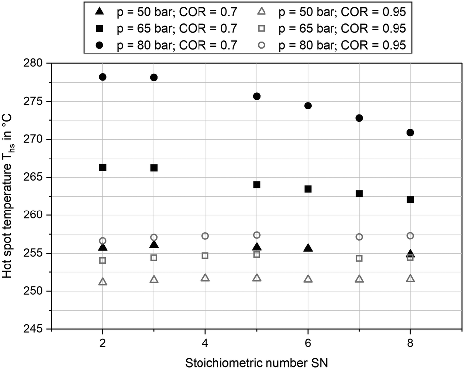 | ||
| Fig. 6 Hot spot temperature measured at COR = 0.7 (black) and COR = 0.95 (grey) and GHSV = 12000 h−1; pressure levels: 50 bar (triangle), 65 bar (diamond) and 80 bar (circle). | ||
At COR = 0.7 an increase of SN led towards a decrease of hot spot temperature at 65 bar and 80 bar, whereas it was almost constant at 50 bar. This can be explained by chemical equilibrium of methanol synthesis decreasing by rising SN and temperature as well as the acceleration of reaction kinetics at increased temperature and pressure. Most probably hot spot temperature was limited by chemical equilibrium at 65 bar and 80 bar when SN exceeded a value of 3.0. As temperature downstream the hot spot approaches cooling temperature and therefore higher equilibrium conversions at simultaneously slower reaction kinetics, the difference between equilibrium and measured molar fractions in Fig. 5 can be explained. While at COR = 0.7 an increase of synthesis pressure from 50 bar to 65 bar as well as from 65 bar to 80 bar increased the hot spot temperature over at least 7 K, at COR = 0.95 only a small rise of hot spot temperature for less than 3.5 K was measured. Moreover, sensitivity towards SN was weaker at COR = 0.95 with the highest hot spot temperature obtained at SN = 5.0 for all three pressure levels. Overall, the sensitivities of hot spot temperatures towards COR and SN are in good agreement to the results of our previous study, where the effect of feed gas composition towards temperature profile inside the reactor was discussed.27
NMR side-product analysis of the liquid product showed the presence of low concentrations of ethanol, propanol and formic acid, which is in good agreement to Göhna et al. who analysed the side-products of CO2-based methanol synthesis.71 However, as non-condensable side-products as methane and DME could not be trapped inside the liquid phase, no comprehensive analysis could be drawn from the liquid phase measurements executed. Further side-product gas phase measurements utilizing a FTIR with a longer optical path length to identify possible traces of these components could be applied in future studies.
Overall, the experimental results obtained from the miniplant setup were plausible regarding the trends in hot spot temperature and product composition. Therefore, the authors are confident that the measured data provides a reliable data basis for the validation and adjustment of kinetic models.
Validation of literature kinetics
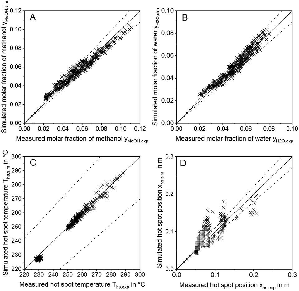
In order to discuss the ability of literature kinetic models for a description of the measured data obtained from the miniplant setup, reactor simulations using the kinetic models as proposed by Graaf,42 Bussche15 and in our previous study, hereon denoted Nestler,27 were performed for all experimental working points. For the sake of clarity, the kinetic models with the parameter set applied as published in literature are hereon labelled with the index “original”. In Fig. 7 parity plots for the three models are provided for the product molar fractions of methanol (A) and water (B) as well as hot spot temperature (C) and position (D), with a confidence interval of 10%. The graphs for the outlet molar fraction of water and methanol show a high level of agreement between experiment and simulation in terms of the kinetic model Nestleroriginal. The models Busscheoriginal and Graaforiginal, however, show strong deviations from the experiments with the tendency of underestimated reaction kinetics.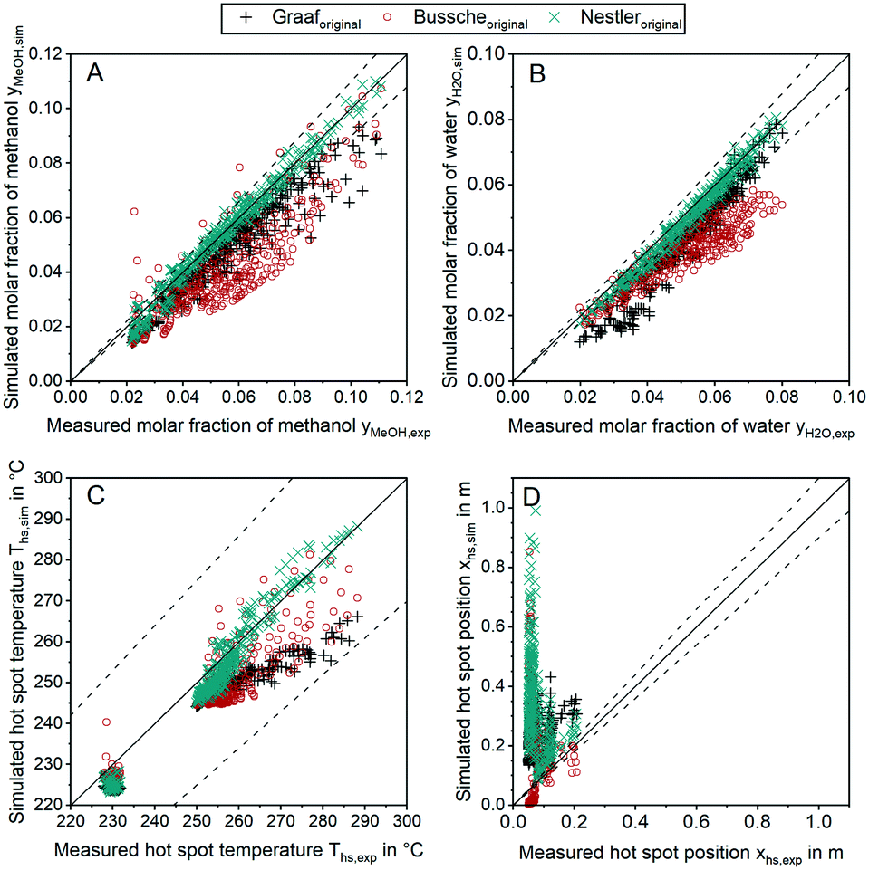 | ||
| Fig. 7 Parity plots for the outlet molar fractions of methanol (A), outlet molar fraction of water (B), hot spot temperature (C) and axial hot spot position (D) including error lines for 0% (solid line) and for 10% (dashed line); experiments were carried out at the miniplant setup; simulation was carried out using the kinetic models by Graaf (+), Bussche (o) and Nestler (x) as published. | ||
Interestingly, none of the models considered in Fig. 7 was able to precisely describe the thermal behaviour of the reactor. Even though the hot spot temperatures of all kinetic models lie within the 10% confidence interval, position of the hot spot was estimated further downstream in the catalyst bed for all kinetic models considered here. In Table 6 the objective function obtained from eqn (35) is shown for the three original models considered in this study together with the respective RMSE-values.
| Parameter | Unit | Graaforiginal | Busscheoriginal | Nestleroriginal |
|---|---|---|---|---|
| f(x) | — | 52.06 | 59.54 | 24.25 |
| RMSET,profile | K | 2.3 | 2.5 | 2.6 |
| RMSET,hs | K | 9.2 | 8.4 | 4.0 |
| RMSEy | % | 0.79 | 1.18 | 0.27 |
The RMSE values of the product composition prove the high accuracy of the Nestleroriginal model for calculation of the product composition in comparison to the literature standards Graaforiginal and Busscheoriginal. While these models predict product composition with a mean error of 0.79% and 1.18%, respectively, a smaller mean error of 0.22% is obtained when the Nestleroriginal model is applied. However, hot spot temperature of this model is still predicted with a mean error of 4 K. As the temperature profile is coupled with the conversion of synthesis gas towards methanol, wrong outlet concentrations could be calculated when the kinetic models discussed in this section are transferred towards different reactor geometries, working conditions or even other reactor types, e.g. an adiabatic quench bed reactor. Even though, the kinetic model previously published by our group delivers a satisfactory description of the outlet concentration for the experimental conditions applied, high deviations could be the case, especially when the kinetic model is used for high COR and higher GHSV. This finding emphasises the necessity for a highly resolved axial measurement in experimental kinetic campaigns, analogous to the temperature profile along the reactor as presented in this work. Moreover, an accurate prediction of the temperature profile is necessary for reactor design, especially when syngas with higher CO contents leading to higher hot spot temperatures is fed to the reactor.
Fitted kinetic models
In order to enhance the applicability of the kinetic models described previously, their semi-empirical parameters (see eqn (20) and (21)) were fitted to the experimental results measured at the miniplant. The parameter fitting was subjected to the weighting factors in eqn (35). Other weighting factors could influence the fitting result along the Pareto front of the optimization problem.72 The kinetic models refitted to the experimental data will be denoted with the index “fit” hereafter.In Table 7 the results of the parameter fitting utilizing the previously defined weight factors are listed by means of the objective function and the respective RMSE values.
| Parameter | Unit | Graaffit | Busschefit | Nestlerfit |
|---|---|---|---|---|
| f(x) | — | 17.50 | 24.97 | 17.93 |
| RMSET,profile | K | 1.4 | 1.8 | 1.5 |
| RMSET,hs | K | 1.7 | 3.4 | 1.8 |
| RMSEy | % | 0.38 | 0.45 | 0.38 |
Comparison of the fitted kinetic models shows comparable remaining errors for the models Graaffit and Nestlerfit, while for the model Busschefit larger deviations remain for temperature profile and product concentration. This can be explained by the reaction mechanisms and rds of the kinetic models. Graaffit and Nestlerfit rely on a common mechanism and similar rds, however with Nestlerfit not considering CO-hydrogenation. In contrast, Bussche's rate equation is based on a different mechanism. Due to the high remaining errors after the parameter fitting (compare Table 7) the rate equations of the Bussche-model were found not applicable for the description of methanol synthesis kinetics on the catalyst considered in this study.
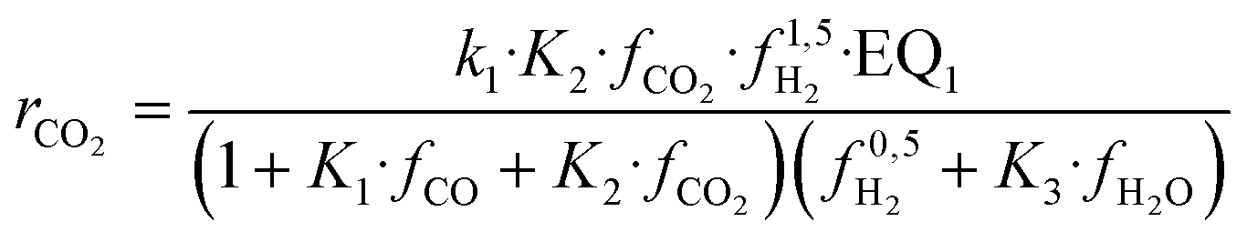
The remaining RMSE values show that the fitted models Graaffit and Nestlerfit predict the temperature profile with a mean error of 1.4 K or 1.5 K, respectively, and therefore with a higher accuracy than the original literature models. A deeper look into the reaction velocities of the fitted kinetic models at Tcool = 240 °C over the whole considered parameter range showed, that CO-hydrogenation of the Graaffit model can be neglected due to a very small reaction rate (|rCO | < 6.0 × 10⁻⁸ mol s−1 kgcat−1) obtained in comparison to CO2-hydrogenation (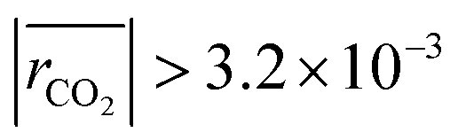 mol s−1 kgcat−1) and rWGS (
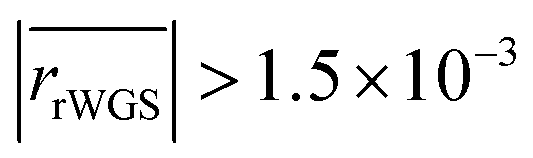 mol s−1 kgcat−1). Due to this finding, it can be stated, that CO-hydrogenation can be neglected for the description of the kinetic behaviour inside the reactor, which is in good agreement to the findings of the scientific community.11,12 Consequently, the kinetic model Nestlerfit will be used throughout the following discussion of this publication.
The set of fitted kinetic parameters for the proposed kinetic model based on the rate equations of eqn (16) and (17) is given in Table 8. The parameter sets of the other kinetic models fitted to the experimental data are provided in the supplementary material.
| Unit | Proposed kinetic parameters | |
|---|---|---|
| k 1 | mol kg−1 s−1 Pa−1 |
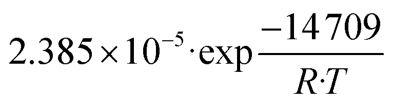
|
| k 2 | mol kg−1 s−1 Pa−0.5 |
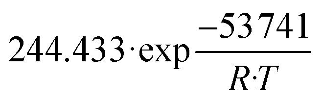
|
| K 1 | Pa−1 |
|
| K 2 | Pa−1 | 4.223 × 10⁻⁶ |
| K 3 | Pa−0.5 |
|
In Fig. 8 the parity plots for the outlet concentrations of methanol (A), water (B) as well as the hot spot temperature (C) and position (D) simulated with the proposed model are provided. The graphs indicate that the description of both, hot spot position and temperature were improved significantly in comparison to the original model (compare Fig. 7). However, while the description of the temperature profile was enhanced with the proposed model, a slightly higher error can be observed regarding the composition of the products methanol and water. This is most likely due to inaccuracies in the measurements of axial temperature profile and product composition. Besides, the remaining error could be a consequence of inaccuracies in the reactor model, e.g. the diffusion or heat transfer sub-models. Application of the validation methodology presented within this study to other reactor geometries could help identifying possible simulation issues and improve the simulation platform.
 | ||
| Fig. 8 Parity plots of the refitted kinetic model Nestlerfit for outlet molar fractions of methanol (A), outlet molar fraction of water (B), hot spot temperature (C) and axial hot spot position (D) including error lines for 0% (solid line) and for 10% (dashed line); experiments were carried out at the miniplant setup. | ||
Despite the slightly lower accuracy of the proposed model in comparison to Nestleroriginal for the calculation of product composition, it is worth pointing out, that the correct description of reaction kinetics along the reactor is vital to enable a reliable transfer of the kinetic model towards industrial scale. To the best of the authors' knowledge, the herein proposed kinetic model delivers such a description and is therefore of a high value for such reactor design problems. However, the validity of the herein proposed kinetic model was only confirmed within the parameter range applied for the experimental campaign (compare Table 5). Expansion of the validated parameter range should only be applied with caution;27 More experimental data will be obtained from the miniplant for a wider and industrially relevant validity range in future work.
Impact on industrial scale
To quantify the behaviour of the herein proposed kinetic model on the industrial scale, a comprehensive simulation study was executed. As our previously published kinetic model27 was based on a similar catalyst, though exclusively based on the measurement of the outlet concentration of a kinetic reactor,27 comparison to this model is capable of showing the impact of the herein proposed validation approach. In Fig. 9 industrial reactor simulations applying both, our previous kinetic model Nestleroriginal and the proposed adapted kinetic model Nestlerfit are compared by means of hot spot temperature (A and B) and position (C and D) as well as methanol (E and F) and water outlet molar fraction (G and H) at synthesis pressures of 50 bar (left side) and 80 bar (right side). The graphs A and B indicate a lower sensitivity of the Nestlerfit model with regard to the dependency of hot spot position and temperature towards COR in comparison to Nestleroriginal. While hot spot temperatures of both models are comparable at COR = 0.8 the proposed kinetic model shows lower hot spot temperatures at COR = 0.7 and increased temperatures at higher COR.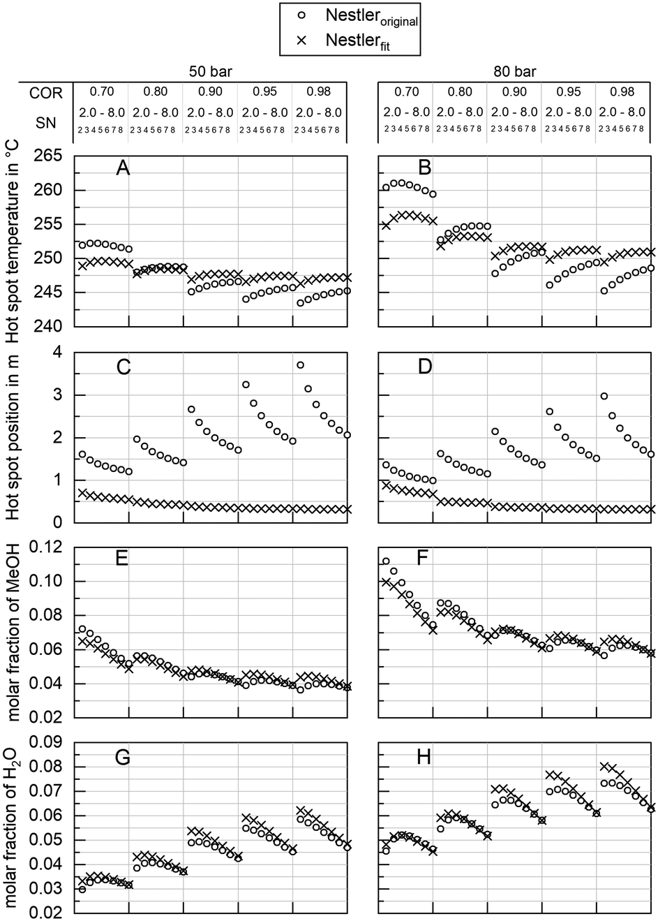 | ||
| Fig. 9 Sensitivity study discussing the behaviour of Nestleroriginal kinetic model (o) and the herein proposed model Nestlerfit (x) by means of hot spot temperature (A and B), hot spot position (C and D), product molar fraction of methanol (E and F) and product molar fraction of water (G and H) at a synthesis pressure of 50 bar (A, C, E and G) and 80 bar (B, D, F and H) in the range 0.7 ≤ COR ≤ 0.98, 2.0 ≤ SN ≤ 8.0 at GHSV = 6000 h−1. | ||
As expected from the comparison of the parity plots of Nestleroriginal model and Nestlerfit model in Fig. 7 and Fig. 8, respectively, high deviations between the kinetic models are observed with regard to hot spot position. This shows that large inaccuracies on the industrial reactor scale can be obtained with kinetic models derived from experimental data measured in traditional integral reactors. Differential measurement of concentration or, as presented here, highly resolved temperature measurements add information to the data set which are advantageous when a transfer from lab to industrial scale is performed. Looking at the product molar fraction of methanol (E and F) and water (G and H) increasing deviations between the two models are present with decreasing SN. This is probably due to larger deviations in hot spot position predicted with decreasing SN. On the one hand this finding again shows the importance of the interlink between a correct kinetic axial description and accurate calculation of product formation. On the other hand, detailed knowledge of the product composition at the reactor exit is of high importance, when the synthesis reactor is embedded in a loop process.
Optimal design for the miniplant setup
In order to optimise the miniplant geometry for an improved agreement between industrial and miniplant scale, scale down from industrial scale to the miniplant dimensions was repeated applying the Nestlerfit kinetic model. In Fig. 10 the optimised reactor diameters determined at GHSV = 9000 h−1 and the pressure levels of 50 bar (A) and 80 bar (B) are shown in a 2D contour plot. The graphs indicate that scale down of the industrial reactor to miniplant scale is correlated to the working range applied. While pressure and COR reveal higher sensitivities towards optimal reactor dimensions, SN does affect the diameter less significantly. With regard to the methodology applied an inner reactor diameter of 9 mm ≤ din ≤ 12 mm would be beneficial for the miniplant setup to improve the similarity towards the industrial reactor scale. Moreover, the smaller reactor diameter would lead to a better heat removal from the reactor and consequently enable the setup to be used for syngas with lower COR. However, wall effects (eqn (31)) as well as other relevant design criteria28 must be considered when the geometry of the miniplant reactor is changed to the dimension proposed here.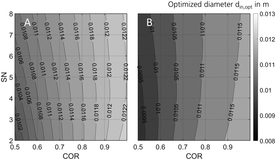 | ||
| Fig. 10 Optimised miniplant reactor diameter over COR and SN at GHSV = 9000 h1 and Tcool = 240 °C for maximised comparability towards industrial scale at 50 bar (A) and 80 bar (B). | ||
As the implementation of Thiele modulus for the description of the diffusion showed to significantly influence the results of the scale down, further research will be necessary in order to validate the diffusion model against experimental data. This could be done by introduction of larger catalyst particles into the miniplant reactor in future work.
Capability of the miniplant for the dynamic reactor analysis
Besides steady state validation, the miniplant setup introduced within this work clearly provides the opportunity to validate reaction kinetics under transient conditions, i.e. fluctuating gas quantity or composition. In Fig. 11 the change in the reactor's temperature profile during an exemplary load change at a pressure level of 80 bar and Tcool = 240 °C from COR = 0.8; SN = 2.0; GHSV = 6000 h−1 towards COR = 0.9; SN = 4.0; GHSV = 12000 h−1 is shown. The graph indicates the displacement of the hot spot inside the reactor further upstream and the decrease of hot spot temperature as a consequence of the increased CO2 content in the feed gas. Further studies are planned in order to validate the dynamic behaviour of the miniplant reactor by a dynamic reactor simulation.
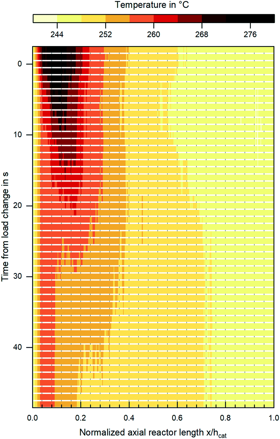 | ||
| Fig. 11 Change in temperature profile during a dynamic load change at a pressure level of 80 bar and Tcool = 240 °C from COR = 0.8; SN = 2.0; GHSV = 6000 h−1 towards COR = 0.9; SN = 4.0; GHSV = 12000 h−1; the load change was applied to the reactor at t = 0 s. | ||
Conclusions
In this study, a novel approach for kinetic model validation and parameter estimation using experimental data from a miniplant setup featuring a highly resolved fibre optic temperature profile in a polytropic miniplant in combination with FTIR product composition measurement was presented.The experimental data obtained from the miniplant reactor are highly correlated to an industrial scale reactor according to the simulation platform applied in this work. Comparison of the experimental data to the reactor simulation of the miniplant using different kinetic models from literature showed the validity of our previously published kinetic model27 by means of the product gas composition. However, comparison of the temperature profiles obtained by reactor simulation towards the experimental data proved the necessity for highly resolved axial measurement to obtain a satisfactory kinetic description. A parameter fitting minimizing the deviation between the experimental data and the simulation was carried out for the rate equations proposed by Graaf,13 Bussche15 and Nestler.27 Remaining discrepancies between the adapted model by Bussche and the experimental data proved that the rate equation proposed by the authors is not capable of describing the reaction kinetics of the catalyst analysed in this work. In contrast, the refitted models by Graaf and Nestler showed a similar quality for the description of the reaction kinetics. As the reaction rate of CO-hydrogenation of the refitted Graaf model was by orders of magnitude below that of CO2-hydrogenation, it can be concluded that the combination of rWGS and CO2-hydrogenation is sufficient for the kinetic description in the parameter range considered. Based on the kinetic rate equation formulated within our previous work,27 a new data set of kinetic parameters was fitted.
A sensitivity analysis performed in the valid parameter range of the herein proposed kinetic model proved the advantage of the herein proposed methodology over classic kinetic fixed bed measurements for scale-up to an industrial reactor. In order to obtain even higher comparability of the miniplant towards industrial scale, the diameter of the miniplant reactor could be adapted in future work based on the simulation-based scale down presented in this work utilizing the updated kinetic model proposed within this study.
Moreover, the data obtained from the miniplant setup was found highly promising for the analysis of a dynamically operated polytropic methanol synthesis reactor. Further work will be carried out to validate a dynamic reactor model against experimental data obtained under transient conditions.
Key issues in our work arise from catalyst deactivation during the experimental study. Validation and adaption of deactivation models using the miniplant setup are important tasks to increase the accuracy of the herein proposed methodology in future work. Moreover, application of the methodology for the spatially resolved validation of a diffusion model will be examined.
Even though the proposed kinetic model shows a high level of agreement towards the experimental data, further research regarding a more appropriate mechanistic description of methanol synthesis could be helpful to deliver an even better description of the reaction kinetics. The authors are confident that the herein applied experimental setup will be a helpful tool in order to clarify the mechanistic nature of methanol synthesis in future work.
To the best of the authors' knowledge the herein proposed novel approach for the validation of reaction kinetics of fixed bed reactions is a significant improvement as it offers an enhanced methodology for bridging between experimental and industrial reactors. Further studies could be carried out transferring this methodology towards other fixed bed syntheses. Moreover, the consideration of radial effects by a two-dimensional simulation could positively affect the quality of the kinetic model obtained and should therefore be investigated in subsequent work.
Nomenclature
| A | Cross sectional area [m2] |
| A k,i | Pre-exponential factor of reaction rate constant ki [variable unit] |
| A K,i | Pre-exponential factor of adsorption constant ki [variable unit] |
| B k,i | Activation energy of reaction rate constant ki [J mol−1] |
| B K,i | Adsorption enthalpy of compontent i [J mol−1] |
| Bo | Bodenstein number [—] |
| c p,f | Molar heat capacity of fluid phase [J mol−1 K−1] |
| COR | Carbon oxide ratio [—] |
| d | Diameter [m] |
| D ax | Axial diffusion coefficient [m2 s−1] |
| D i,j | Binary diffusion coefficient of component i and j [m2 s−1] |
| D K,i | Knudsen diffusion coefficient of component i [m2 s−1] |
| D em,i | Effective diffusion coefficient of component i [m2 s−1] |
| EoS | Equation of State |
| GHSV | Gas hourly space velocity [h−1] |
| h cat | Height of catalyst bed [m] |
| ΔH0R | Enthalpy of formation under standard condition [kJ mol−1] |
| k i | Reaction rate constant of reaction i [variable unit] |
| Pseudo first order reaction rate constant [mol s−1 m−3 Pa−1] |
| K i | Adsoption constant of component i [variable unit] |
| K eq,i | Equilibrium constant of reaction i [variable unit] |
| Pseudo equilibrium constant [—] |
| ṅ | Molar flow [mol s−1] |
| N | Number [—] |
| p | Pressure [Pa] |
| r eff,i | Particle reaction velocity of reaction i [mol kg−1 s−1] |
| r i | Intrinsic reaction velocity of reaction i [mol kg−1 s−1] |
| R | Universal gas constant [J mol−1 K−1] |
| rds | Rate determining step |
| Rep | Particle Reynolds number [—] |
| RMSE | Root mean square error |
| rWGS | Reverse water-gas-shift reaction |
| SN | Stoichiometric number [—] |
| SRK | Soave–Redlich–Kwong |
| STY | Space time yield [kgMeOH Lcat−1 s−1] |
| t | Time [s] |
| T | Temperature [K] |
| u 0 | Empty tube gas velocity [m s−1] |
| U | Heat transfer coefficient [W m−2 K−1] |
|
| Volumetric flow rate [m3 h−1] |
| V | Volume [m3] |
| WGS | Water-gas-shift reaction |
| x | Axial length [m] |
| y i | Molar fraction of component [—] |
Greek letters
| α | Weight factor of temperature profile RMSE [K−1] |
| β | Weight factor of hot spot RMSE [K−1] |
| γ | Weight factor of molar fraction RMSE [—] |
| ε | Porosity [—] |
| η eff,i | Efficiency factor of reaction i [—] |
| λ | Heat conduction coefficient [W m−1 K−1] |
| ν j | Stoichiometric factor of component j [—] |
| ρ | Density [kg m−3] |
| τ | Tortuosity of the catalyst particle [—] |
| ν | Kinematic viscosity [m2 s−1] |
| φ | Reactor-particle diameter ratio [—] |
| ϕ M,i | Thiele modulus [—] |
Indices
| bulk | Bulk phase |
| cat | Catalyst in the reactor |
| comp | Component |
| cool | Cooling medium |
| data pt | Data points |
| exp | Experimental |
| ext | External |
| f | Fluid phase |
| (g) | Gas phase |
| H2 | Hydrogen |
| H2O | Water |
| hs | Hot spot |
| inc | Increment |
| ind | Industrial scale |
| int | Internal |
| MeOH | Methanol |
| miniplant | Miniplant scale |
| norm | Norm conditions |
| p | Particle |
| profile | Profile |
| rad | Radial |
| sim | Simulated |
| wall | Wall |
| T | Temperature |
| tot | total |
| x | Axial dimension |
| y | Molar fraction |
Conflicts of interest
There are no conflicts to declare.Acknowledgements
This work was carried out in the framework of the “PtM – Power-to-Methanol” project funded by the German Federal Ministry of Economic Affairs and Energy (03ET6140F). The partners of the PtM consortium are kindly acknowledged for their scientific input throughout the runtime of the project. Special thanks are dedicated to Clariant for the provision of the methanol synthesis catalyst. Melanie Iwanow and Marion Wölbing from Fraunhofer IGB are kindly acknowledged for the NMR analysis of the liquid product. Among the team of Hydrogen Division at Fraunhofer Institute for Solar Energy Systems ISE special thanks are dedicated to Johannes Full, Sebastian Schäfer and Marco Tranitz for their technical support designing, building, and commissioning the miniplant setup. Finally, Deutsche Bundesstiftung Umwelt (DBU) is kindly acknowledged for the funding of the work of Florian Nestler (20017/517).Notes and references
- C. Hank, A. Sternberg, N. Köppel, M. Holst, T. Smolinka, A. Schaadt, C. Hebling and H.-M. Henning, Sustainable Energy Fuels, 2020, 4(5), 2256 RSC.
- E. Bargiacchi, M. Antonelli and U. Desideri, Energy, 2019, 183, 1253 CrossRef CAS.
- M. Berggren, Global Methanol - State of the Industry, Frankfurt am Main, 2019 Search PubMed.
- F. Nestler, M. Krüger, J. Full, M. J. Hadrich, R. J. White and A. Schaadt, Chem. Ing. Tech., 2018, 90, 1409 CrossRef CAS.
- M. Götz, J. Lefebvre, F. Mörs, A. McDaniel Koch, F. Graf, S. Bajohr, R. Reimert and T. Kolb, Renewable Energy, 2016, 85, 1371 CrossRef.
- A. Zurbel, M. Kraft, S. Kavurucu-Schubert and M. Bertau, Chem. Ing. Tech., 2018, 90, 721 CrossRef CAS.
- J. Schittkowski, H. Ruhland, D. Laudenschleger, K. Girod, K. Kähler, S. Kaluza, M. Muhler and R. Schlögl, Chem. Ing. Tech., 2018, 90, 1419 CrossRef CAS.
- V. Dieterich, A. Buttler, A. Hanel, H. Spliethoff and S. Fendt, Energy Environ. Sci., 2020, 13(10), 3207 RSC.
- Y. Slotboom, M. J. Bos, J. Pieper, V. Vrieswijk, B. Likozar, S. Kersten and D. Brilman, Chem. Eng. J., 2020, 389, 124181 CrossRef CAS.
- G. Bozzano and F. Manenti, Prog. Energy Combust. Sci., 2016, 56, 71 CrossRef.
- M. Sahibzada, I. S. Metcalfe and D. Chadwick, J. Catal., 1998, 174, 111 CrossRef CAS.
- G. C. Chinchen, P. J. Denny, D. G. Parker, M. S. Spencer and D. A. Whan, Appl. Catal., 1987, 30, 333 CrossRef CAS.
- G. H. Graaf, E. J. Stamhuis and A. Beenackers, Chem. Eng. Sci., 1988, 43, 3185 CrossRef CAS.
- K. Klier, J. Catal., 1982, 74, 343 CrossRef CAS.
- K. M. Vanden Bussche and G. F. Froment, J. Catal., 1996, 161, 1 CrossRef CAS.
- C. Seidel, A. Jörke, B. Vollbrecht, A. Seidel-Morgenstern and A. Kienle, Chem. Eng. Sci., 2018, 175, 130 CrossRef CAS.
- N. Park, M.-J. Park, Y.-J. Lee, K.-S. Ha and K.-W. Jun, Fuel Process. Technol., 2014, 125, 139 CrossRef CAS.
- K. Kobl, S. Thomas, Y. Zimmermann, K. Parkhomenko and A.-C. Roger, Catal. Today, 2016, 270, 31 CrossRef CAS.
- D. Rahman, Kinetic Modeling Of Methanol Synthesis From Carbon Monoxide, Carbon Dioxide, And Hydrogen Over A Cu/ZnO/Cr2O3 Catalyst, Masterthesis, San Jose State University, 2012 Search PubMed.
- M. Peter, M. B. Fichtl, H. Ruhland, S. Kaluza, M. Muhler and O. Hinrichsen, Chem. Eng. J., 2012, 203, 480 CrossRef CAS.
- L. Chen, Q. Jiang, Z. Song and D. Posarac, Chem. Eng. Technol., 2011, 34, 817 CrossRef CAS.
- J. J. Meyer, P. Tan, A. Apfelbacher, R. Daschner and A. Hornung, Chem. Eng. Technol., 2016, 39, 233 CrossRef CAS.
- A. Montebelli, C. G. Visconti, G. Groppi, E. Tronconi, C. Ferreira and S. Kohler, Catal. Today, 2013, 215, 176 CrossRef CAS.
- F. Manenti and G. Bozzano, Ind. Eng. Chem. Res., 2013, 52, 13079 CrossRef CAS.
- F. Manenti, S. Cieri, M. Restelli and G. Bozzano, Comput. Chem. Eng., 2013, 48, 325 CrossRef CAS.
- F. Manenti, S. Cieri and M. Restelli, Chem. Eng. Sci., 2011, 66, 152 CrossRef CAS.
- F. Nestler, A. R. Schütze, M. Ouda, M. J. Hadrich, A. Schaadt, S. Bajohr and T. Kolb, Chem. Eng. J., 2020, 394, 124881 CrossRef CAS.
- J. Pérez-Ramírez, Catal. Today, 2000, 60, 93 CrossRef.
- D. A. Hickman, J. C. Degenstein and F. H. Ribeiro, Curr. Opin. Chem. Eng., 2016, 13, 1 CrossRef.
- R. J. Berger, J. Pérez-Ramírez, F. Kapteijn and J. A. Moulijn, Appl. Catal., A, 2002, 227, 321 CrossRef CAS.
- VDI-Wärmeatlas: Mit 320 Tabellen, ed. P. Stephan, Springer Vieweg, Berlin, 2013 Search PubMed.
- A. Jess and P. Wasserscheid, Chemical technology: An integral textbook, Wiley-VCH, Weinheim, 2013 Search PubMed.
- T. Henkel, Modellierung von Reaktion und Stofftransport in geformten Katalysatoren am Beispiel der Methanolsynthese, PhD thesis, TU München, 2011 Search PubMed.
- A. Keshavarz, A. Mirvakili, S. Chahibakhsh, A. Shariati and M. R. Rahimpour, Chem. Eng. Process.: Process Intesif., 2020, 158, 108176 CrossRef CAS.
- P. Maksimov, A. Laari, V. Ruuskanen, T. Koiranen and J. Ahola, RSC Adv., 2020, 10, 23690 RSC.
- M. Khanipour, A. Mirvakili, A. Bakhtyari, M. Farniaei and M. R. Rahimpour, Int. J. Hydrogen Energy, 2020, 45(12), 7386 CrossRef CAS.
- F. Samimi, M. Feilizadeh, M. Ranjbaran, M. Arjmand and M. R. Rahimpour, Fuel Process. Technol., 2018, 181, 375 CrossRef CAS.
- X. Cui and S. K. Kær, Chem. Eng. J., 2020, 124632 CrossRef CAS.
- G. Leonzio, E. Zondervan and P. U. Foscolo, Int. J. Hydrogen Energy, 2019, 44(16), 7915 CrossRef CAS.
- S. Ghosh, V. Uday, A. Giri and S. Srinivas, J. Cleaner Prod., 2019, 217, 615 CrossRef CAS.
- R. O. D. Santos, L. D. S. Santos and D. M. Prata, J. Cleaner Prod., 2018, 186, 821 CrossRef.
- G. H. Graaf, H. Scholtens, E. J. Stamhuis and A. Beenackers, Chem. Eng. Sci., 1990, 45, 773 CrossRef CAS.
- G. H. Graaf, The synthesis of methanol in gas-solid and gas-slurry reactors, PhD thesis, University of Groningen, 1988 Search PubMed.
- G. H. Graaf and J. G. M. Winkelman, Ind. Eng. Chem. Res., 2016, 55, 5854 CrossRef CAS.
- G. Soave, Chem. Eng. Sci., 1972, 27, 1197 CrossRef CAS.
- G. F. Froment and L. H. Hosten, Catalytic Kinetics Modelling, Springer, Berlin, Heidelberg, New York, 1981, p. 97 Search PubMed.
- J. Solsvik and H. A. Jakobsen, Chem. Eng. Sci., 2011, 66, 1986 CrossRef CAS.
- S. Lee, Methanol synthesis technology, CRC Press, Boca Raton, Fla., 1990 Search PubMed.
- E. W. Thiele, Ind. Eng. Chem., 1939, 31, 916 CrossRef CAS.
- B. J. Lommerts, G. H. Graaf and A. Beenackers, Chem. Eng. Sci., 2000, 55, 5589 CrossRef CAS.
- S. Abrol and C. M. Hilton, Comput. Chem. Eng., 2012, 40, 117 CrossRef CAS.
- K. R. Westerterp, W. P. van Swaaij, A. Beenackers and H. Kramers, Chemical reactor design and operation, Wiley, Chichester et al, 1984 Search PubMed.
- E. N. Fuller, P. D. Schettler and J. C. Giddings, Ind. Eng. Chem., 1966, 58, 18 CrossRef CAS.
- DIPPR 801 Database, https://dippr.aiche.org Search PubMed.
- H. Kordabadi and A. Jahanmiri, Chem. Eng. J., 2005, 108, 249 CrossRef CAS.
- A. Elkamel, G. Reza Zahedi, C. Marton and A. Lohi, Energies, 2009, 2, 180 CrossRef CAS.
- N. Rezaie, A. Jahanmiri, B. Moghtaderi and M. R. Rahimpour, Chem. Eng. Process.: Process Intesif., 2005, 44, 911 CrossRef CAS.
- F. M. Dautzenberg, in Deactivation and Testing of Hydrocarbon-Processing Catalysts, ed. J. P. O'Connell, T. Takatsuka and G. L. Woolery, American Chemical Society, Washington, DC, 1996, p. 99 Search PubMed.
- S. T. Sie, in Deactivation and Testing of Hydrocarbon-Processing Catalysts, ed. J. P. O'Connell, T. Takatsuka and G. L. Woolery, American Chemical Society, Washington, DC, 1996, p. 6 Search PubMed.
- M. Kraume, Transportvorgänge in der Verfahrenstechnik, Springer, Berlin Heidelberg, Berlin, Heidelberg, 2012 Search PubMed.
- M. Zlokarnik, Scale-Up in Chemical Engineering, Wiley, 2006 Search PubMed.
- G. Damköhler and G. Delcker, Z. Elektrochem. Angew. Phys. Chem., 1938, 44, 1938 Search PubMed.
- G. C. Chinchen, P. J. Denny, J. R. Jennings, M. S. Spencer and K. C. Waugh, Appl. Catal., 1988, 36, 1 CrossRef CAS.
- J. A. Nelder and R. Mead, Comput. J., 1965, 7, 308 CrossRef.
- J. Schwarz and D. Samiec, Proceedings Sensor, 2017, 2017, p. 212 Search PubMed.
- X. Zhou, C. Yang and W. Gui, J. Ind. Manag. Optim., 2012, 8, 1039 Search PubMed.
- A. Savitzky and M. J. E. Golay, Anal. Chem., 1964, 36, 1627 CrossRef CAS.
- M. B. Fichtl, D. Schlereth, N. Jacobsen, I. Kasatkin, J. Schumann, M. Behrens, R. Schlögl and O. Hinrichsen, Appl. Catal., A, 2015, 502, 262 CrossRef CAS.
- J. T. Sun, I. S. Metcalfe and M. Sahibzada, Ind. Eng. Chem. Res., 1999, 38, 3868 CrossRef CAS.
- M. Saito and K. Murata, Catal. Surv. Asia, 2004, 8, 285 CrossRef CAS.
- H. Göhna and P. König, CHEMTECH, 1994, 24, 36 Search PubMed.
- D. A. van Veldhuizen and G. B. Lamont, Evol. Comput., 2000, 8, 125 CrossRef CAS PubMed.
Footnote |
| † Electronic supplementary information (ESI) available. See DOI: 10.1039/d1re00071c |
| This journal is © The Royal Society of Chemistry 2021 |