
 Open Access Article
 This Open Access Article is licensed under a Creative Commons Attribution-Non Commercial 3.0 Unported Licence
Study of physical properties of a ferrimagnetic spinel Cu1.5Mn1.5O4: spin dynamics, magnetocaloric effect and critical behavior
Abir Hadded *a,
Jalel Massoudi*a,
Sirine Gharbia,
Essebti Dhahria,
A. Tozrib and
Mohamed R. Berber*c
*a,
Jalel Massoudi*a,
Sirine Gharbia,
Essebti Dhahria,
A. Tozrib and
Mohamed R. Berber*c
aLaboratoire de Physique Appliquée, Faculté des Sciences, Université de Sfax, 3000, Tunisia. E-mail: abir.hadded1994@gmail.com; jalel.massoudi@gmail.com
bPhysics Department, College of Science, Jouf University, Sakaka 2014, Saudi Arabia
cChemistry Department, College of Science, Jouf University, Sakaka 2014, Saudi Arabia
First published on 26th July 2021
Abstract
The present work reports a detailed study of the spin dynamics, magnetocaloric effect and critical behaviour near the magnetic phase transition temperature, of a ferrimagnetic spinel Cu1.5Mn1.5O4. The dynamic magnetic properties investigated using frequency-dependent ac magnetic susceptibility fitted using different phenomenological models such as Neel–Arrhenius, Vogel–Fulcher and power law, strongly indicate the presence of a cluster-glass-like behavior of Cu1.5Mn1.5O4 at 40 K. The magnetization data have revealed that our compound displays an occurrence of second-order paramagnetic (PM) to ferrimagnetic (FIM) phase transition at the Curie temperature TC = 80 K as the temperature decrease. In addition, the magnetic entropy change (ΔSM) was calculated using two different methods: Maxwell relations and Landau theory. An acceptable agreement was found between both sets of data, which proves the importance of both electron interaction and magnetoelastic coupling in the magnetocaloric effect (MCE) properties of Cu1.5Mn1.5O4. The relative cooling power (RCP) reaches 180.13 (J kg−1) for an applied field at 5 T, making our compound an effective candidate for magnetic refrigeration applications. The critical exponents β, γ and δ as well as transition temperature TC were extracted from various techniques indicating that the magnetic interaction in our sample follows the 3D-Ising model. The validity of the critical exponents is confirmed by applying the Windom scaling hypothesis.
1. Introduction
There is a category of double oxides of general formula AB2O4 which includes two types of arrangements. In the first possible distribution, known as normal spinel, the A2+ cations occupy the tetrahedral interstitial sites and the B3+ cations occupy the octahedral sites. This distribution is indicated as (A2+)[B23+]O4 where the parentheses designate the tetrahedral, and the brackets, the octahedral positions. A second possible arrangement, (B3+)[A2+B3+]O4 known as perfectly inverse spinel, is characterized by B cations occupying all of the tetrahedral and half of the octahedral sites, while the other species (A) occupies the remaining (half of the) octahedral sites. Prototypical examples of normal and inverse spinels are MgAl2O4 (space group Fd![[3 with combining macron]](https://www.rsc.org/images/entities/char_0033_0304.gif) m) and MgGa2O4 (space group P4122), respectively.1,2 Otherwise, there are many possible intermediate distributions represented by the formula (A1−i2+Bi3+)[Ai2+B2−i3+]O4, where i denotes the inversion degree. Magnetic spinel oxides have been extensively investigated owing to their physical properties.3 They exhibit various magnetic, dielectric, and optical properties, according to their structures, compositions and cation distributions.4–6 Several cations can be placed in tetrahedral A and octahedral B sites to adjust the magnetic properties. They can present paramagnetic, ferrimagnetic, spin glass and antiferromagnetic behavior, depending on A and B site cations.7,8 Besides, nonmagnetic ions occupying the A or B sites will lead to magnetic frustration, so that one new magnetic phase will be detected, such as semi-spin-glass (SSG), re-entrant spin-glass (RSG) and spin-glass (SG).9–11 The existence of the SG comportment is closely associated with the magnetic frustration,12,13 concluding therefore, that system with lowest energy tend not to be stable.14 In recent years, magnetic materials have attracted increasing interest among a wide range of researchers whose concern has been grown with the investigation of the potential use in various applications, including but not limited magnetocaloric refrigeration,15 magnetically guided drug delivery,16 magnetic resonance imaging (MRI) enhancement,17 ferrofluid technology,18 and high-density information storage.19 Fe3O4 or magnetite, is the most-studied spinel ferrite. Recently, the magnetotransport of magnetite has attracted much attention due to the discovery of giant magnetoresistance (GMR) effective in this material.20 Raman spectroscopy has proven effective in studying the elementary excitation of material. A physical explanation of the enhanced electron–electron correlation in the presence of a magnetic field is proposed to be responsible for the GMR mechanical in magnetite material.21 The dynamics of magnetic superparamagnetic particles have been a subject of intense study in fundamental physics research.22–24 Cluster glass are kind of spin glasses. In CG groups of spins are locally ordered creating small domains which interact between each other similar to single spins in simple spin glass. To distinguish simple SG from CG few points are considered: relative shift per frequency decade of freezing temperature is much lower for CG,25,26 the temperature where ZFC magnetic susceptibility reach maximum (Tmax) and a value of magnetic susceptibility maximum (χmax) strongly depend on applied magnetic field,27 the monotonic increase of FC (χ(T) for field-cooling) line with decreasing temperature is characteristic for CG compounds,27,28 whereas, in simple spin-glass small cusps in the FC behaviour is often visible. The study of magnetic spin behavior is still very limited, which needs to be explored. To our knowledge, until now, no report was available which deals with the relaxation studies of a Cu1.5Mn1.5O4 in a single nanostructure. Many researches have been devoted to the critical behavior of magnetic materials with the aim of reporting a detailed description of the interactions between the spins. Theoretical researches demonstrate that magnetic behavior was described by short-range interactions.29,30 Other researchers have identified that critical exponents are in accord with a long-range exchange interaction model.31 The study of the critical properties has been reported for the first time in the mean field theory.32 But currently, there are 4 different theoretical models that can describe the magnetic interactions. The mean field model (β = 0.5, γ = 1 and δ = 3) describes long-range exchange interactions neglecting critical fluctuations in the vicinity of the Curie temperature TC.31 The 3D Heisenberg model (β = 0.365, γ = 1.336 and δ = 4.80) describes short-range exchange interactions at the occurrence of spin fluctuations near TC.31 In the 3D Ising model (β = 0.325, γ = 1.240 and δ = 4.82), the spins interact with their neighbors that are usually arranged in a lattice, and their magnetic dipolar moments that can be in one of the two states ±1.31 Finally, the tricritical mean field model (β = 0.25, γ = 1 and δ = 5) proposes that the sample's composition should be close to a tri-critical point in the phase diagram of the used material.31 Recently, there has been a swell of interest in materials containing copper and manganese oxides with spinel structures owing to their interesting magnetic properties.33–35 Cu1.5Mn1.5O4 is a typical example, crystallizing with a spinel structure, with cationic distributions [Cu+]A[Cu0.52+Mn1.54+]BO Cu+ of [Ar]3d10 electronic configuration occupies the tetrahedral site A while Cu2+ ([Ar]3d9) and Mn4+ ([Ar]3d3) occupy the octahedral site.36–38 For the Cu1.5Mn1.5O4 system, both the valance states of Cu ions (Cu1+/Cu2+) and Mn ions (Mn4+) and their site occupancies at the tetrahedral (A site) and octahedral (B site) sites have large flexibilities and hence the affecting magnetic properties, it can be justified by superexchange coupling between the sublattices, and the fact that the local ferrimagnetic order of Mn4+ ions on B sites can be disturbed by Cu2+ on the same sites.
m) and MgGa2O4 (space group P4122), respectively.1,2 Otherwise, there are many possible intermediate distributions represented by the formula (A1−i2+Bi3+)[Ai2+B2−i3+]O4, where i denotes the inversion degree. Magnetic spinel oxides have been extensively investigated owing to their physical properties.3 They exhibit various magnetic, dielectric, and optical properties, according to their structures, compositions and cation distributions.4–6 Several cations can be placed in tetrahedral A and octahedral B sites to adjust the magnetic properties. They can present paramagnetic, ferrimagnetic, spin glass and antiferromagnetic behavior, depending on A and B site cations.7,8 Besides, nonmagnetic ions occupying the A or B sites will lead to magnetic frustration, so that one new magnetic phase will be detected, such as semi-spin-glass (SSG), re-entrant spin-glass (RSG) and spin-glass (SG).9–11 The existence of the SG comportment is closely associated with the magnetic frustration,12,13 concluding therefore, that system with lowest energy tend not to be stable.14 In recent years, magnetic materials have attracted increasing interest among a wide range of researchers whose concern has been grown with the investigation of the potential use in various applications, including but not limited magnetocaloric refrigeration,15 magnetically guided drug delivery,16 magnetic resonance imaging (MRI) enhancement,17 ferrofluid technology,18 and high-density information storage.19 Fe3O4 or magnetite, is the most-studied spinel ferrite. Recently, the magnetotransport of magnetite has attracted much attention due to the discovery of giant magnetoresistance (GMR) effective in this material.20 Raman spectroscopy has proven effective in studying the elementary excitation of material. A physical explanation of the enhanced electron–electron correlation in the presence of a magnetic field is proposed to be responsible for the GMR mechanical in magnetite material.21 The dynamics of magnetic superparamagnetic particles have been a subject of intense study in fundamental physics research.22–24 Cluster glass are kind of spin glasses. In CG groups of spins are locally ordered creating small domains which interact between each other similar to single spins in simple spin glass. To distinguish simple SG from CG few points are considered: relative shift per frequency decade of freezing temperature is much lower for CG,25,26 the temperature where ZFC magnetic susceptibility reach maximum (Tmax) and a value of magnetic susceptibility maximum (χmax) strongly depend on applied magnetic field,27 the monotonic increase of FC (χ(T) for field-cooling) line with decreasing temperature is characteristic for CG compounds,27,28 whereas, in simple spin-glass small cusps in the FC behaviour is often visible. The study of magnetic spin behavior is still very limited, which needs to be explored. To our knowledge, until now, no report was available which deals with the relaxation studies of a Cu1.5Mn1.5O4 in a single nanostructure. Many researches have been devoted to the critical behavior of magnetic materials with the aim of reporting a detailed description of the interactions between the spins. Theoretical researches demonstrate that magnetic behavior was described by short-range interactions.29,30 Other researchers have identified that critical exponents are in accord with a long-range exchange interaction model.31 The study of the critical properties has been reported for the first time in the mean field theory.32 But currently, there are 4 different theoretical models that can describe the magnetic interactions. The mean field model (β = 0.5, γ = 1 and δ = 3) describes long-range exchange interactions neglecting critical fluctuations in the vicinity of the Curie temperature TC.31 The 3D Heisenberg model (β = 0.365, γ = 1.336 and δ = 4.80) describes short-range exchange interactions at the occurrence of spin fluctuations near TC.31 In the 3D Ising model (β = 0.325, γ = 1.240 and δ = 4.82), the spins interact with their neighbors that are usually arranged in a lattice, and their magnetic dipolar moments that can be in one of the two states ±1.31 Finally, the tricritical mean field model (β = 0.25, γ = 1 and δ = 5) proposes that the sample's composition should be close to a tri-critical point in the phase diagram of the used material.31 Recently, there has been a swell of interest in materials containing copper and manganese oxides with spinel structures owing to their interesting magnetic properties.33–35 Cu1.5Mn1.5O4 is a typical example, crystallizing with a spinel structure, with cationic distributions [Cu+]A[Cu0.52+Mn1.54+]BO Cu+ of [Ar]3d10 electronic configuration occupies the tetrahedral site A while Cu2+ ([Ar]3d9) and Mn4+ ([Ar]3d3) occupy the octahedral site.36–38 For the Cu1.5Mn1.5O4 system, both the valance states of Cu ions (Cu1+/Cu2+) and Mn ions (Mn4+) and their site occupancies at the tetrahedral (A site) and octahedral (B site) sites have large flexibilities and hence the affecting magnetic properties, it can be justified by superexchange coupling between the sublattices, and the fact that the local ferrimagnetic order of Mn4+ ions on B sites can be disturbed by Cu2+ on the same sites.
The present paper reports that ac susceptibility shows the cluster glass behavior of Cu1.5Mn1.5O4 compound. We identified the magnetic properties of ferrimagnetic spinel Cu1.5Mn1.5O4. The study of magnetocaloric properties has a twofold objective. Firstly, from a fundamental point of view, our sample offers an opportunity to investigate the MCE associated with a magnetic transition. Secondly, from an application point of view, it's considered as a good candidate for the cooling system based on magnetic refrigeration. Furthermore, we will determine the critical exponents β, γ and δ in order to identify the model describing the nature of the magnetic interaction in our sample. To date, no research papers have been devoted to study these properties associated with such compound.
2. Experimental techniques
Cu1.5Mn1.5O4 compound were synthesized by the sol–gel method described in our previous study.39 Low-field ac-susceptibility measurements were made at various frequencies in a temperature range of 20 to 122 K. Magnetic measurements were recorded using a SQUID magnetometer. The magnetization measurements were carried out according to the zero field cooling (ZFC) and field cooling (FC) protocols under 500 Oe and in a temperature range of 20 to 122 K. The isothermal magnetization M (T, H) was recorded for different temperatures under a magnetic field up to 5 T.3. Results and discussions
3.1 Magnetic measurements
Fig. 1a illustrates the variation of the magnetization as a function of temperature for Cu1.5Mn1.5O4 the magnetic measurements of which were carried out under 500 Oe according to the zero field cooling (ZFC) and field cooling (FC) protocols. The magnetization presents two different regions as a function of temperature. At high temperature, the two curves correspond to superimpose and reversible common part. The other at low temperature, in which a maximum in the ZFC magnetization can be observed below the magnetic irreversibility temperature (Tirr). The magnetic behavior is irreversible revealing the magnetic anisotropy.40 For the Cu1.5Mn1.5O4 compound, the obvious bifurcation between the FC and ZFC M–T curves occurs in the irreversible temperature (Tirr). This phenomenon, known as low temperature glassy magnetic state, could be a spin glass,41 a canonical spin glass41,42 or a cluster glass.43 The magnetic transition temperature (TC = 80 K) has been determined using the magnetization derivative dM/dT curve (inset Fig. 1a). A similar behavior was observed in the case of CuMn2O4 system.35,44,45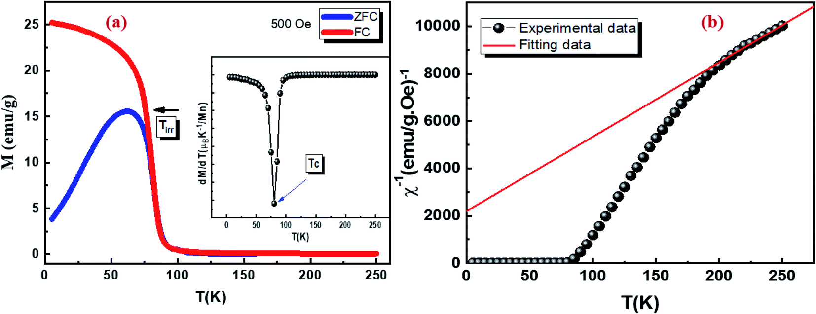 | ||
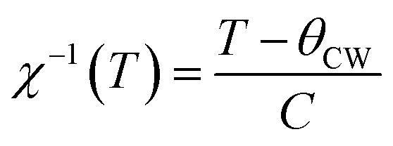
| Fig. 1 Magnetization of Cu1.5Mn1.5O4 after zero-field cooling (ZFC) and during field cooling (FC) acquired under a field of 0.05 T, the inset shows the dM/dT curve as a function of temperature (a). Temperature dependence of the inverse magnetic susceptibility χ−1(T), the solid line is the linear fit to the susceptibility data according to Curie–Weiss law in paramagnetic regime (b). | ||
Aiming to achieve a better understanding of the magnetic behavior of Cu1.5Mn1.5O4 we have plotted the variation of the inverse of magnetic susceptibility as a function of the temperature in the PM region. Fig. 1b display a parabolical variation above 80 K, suggesting the existence of ferrimagnetic behavior (TC = 80 K and θCW = −72 K) due to the anti-parallel order of the magnetic moments of the nearest neighbor of unequal magnitude.46 This result is significantly different from the reported results of Cu1.5Mn1.5O4.47 The synthesized system, using the one-step self-assembly pathway, exhibit ferromagnetic transition phase at room temperature. Therefore the preparation method and the annealing temperature affecting magnetic phase transition.
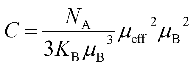
The inverse magnetic susceptibility curve above 80 K has been fitted by the Curie–Weiss law:48
 | (1) |
The obtained fitted parameters values for Cu1.5Mn1.5O4 are θCW = −72 K and C = 3.198. The obtained value of θCW is negative, confirm the FIM character of our compound.
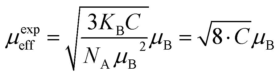
The experimental effective moments can be calculated (in unit of Bohr magneton μB) from the Curie constant using the following relation:49
 | (2) |
In Gaussian CGS units μB = 0.9274 × 10⁻²¹ is the Bohr magneton and KB = 1.38016 × 10⁻¹⁶ erg. K is Boltzmann constant.
In this case μexpeff is written:
 | (3) |
The obtained values of μexpeff is found to be equal to 5.058 μB.
From the cationic distributions [Cu+]A[Cu0.52+Mn1.54+]BO4, the theoretical effective magnetic moment is given by:
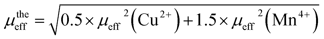 | (4) |
The value of μtheeff is 4.899 μB. This μtheeff is very close to our μexpeff.
The obtained values of TC, C, θCW and μexpeff for our sample are compared with different copper manganese, mixed oxide spinel34,35,50 listed in Table 1.
3.2 Ac susceptibility
The present research paper seeks to gain a better comprehension of the magnetic order state and the dynamic behavior in our sample. We, therefore, commenced by carrying out ac susceptibility measurements under low magnetic fields ranging from 5 Hz to 950 Hz. Fig. 2a exhibits the real part (χ′) of ac susceptibility as a function of the temperature in an ac field of 10 Oe of Cu1.5Mn1.5O4 compound. The curve at each frequency suggests a clear peak at a specific temperature Tf, which is usually taken as the freezing temperature. The magnetic susceptibility χ′(T) presents a clear correlation with the frequency, which is accompanied by a decrease in the intensity of the peak and a shift towards high temperatures as the frequency increases. Such behavior of (χ′) is a typical feature of the spin glass, cluster glass and super paramagnetic systems51 caused by the intra-particle surface spin disorder or by strong magnetostatic interparticle interactions.41,52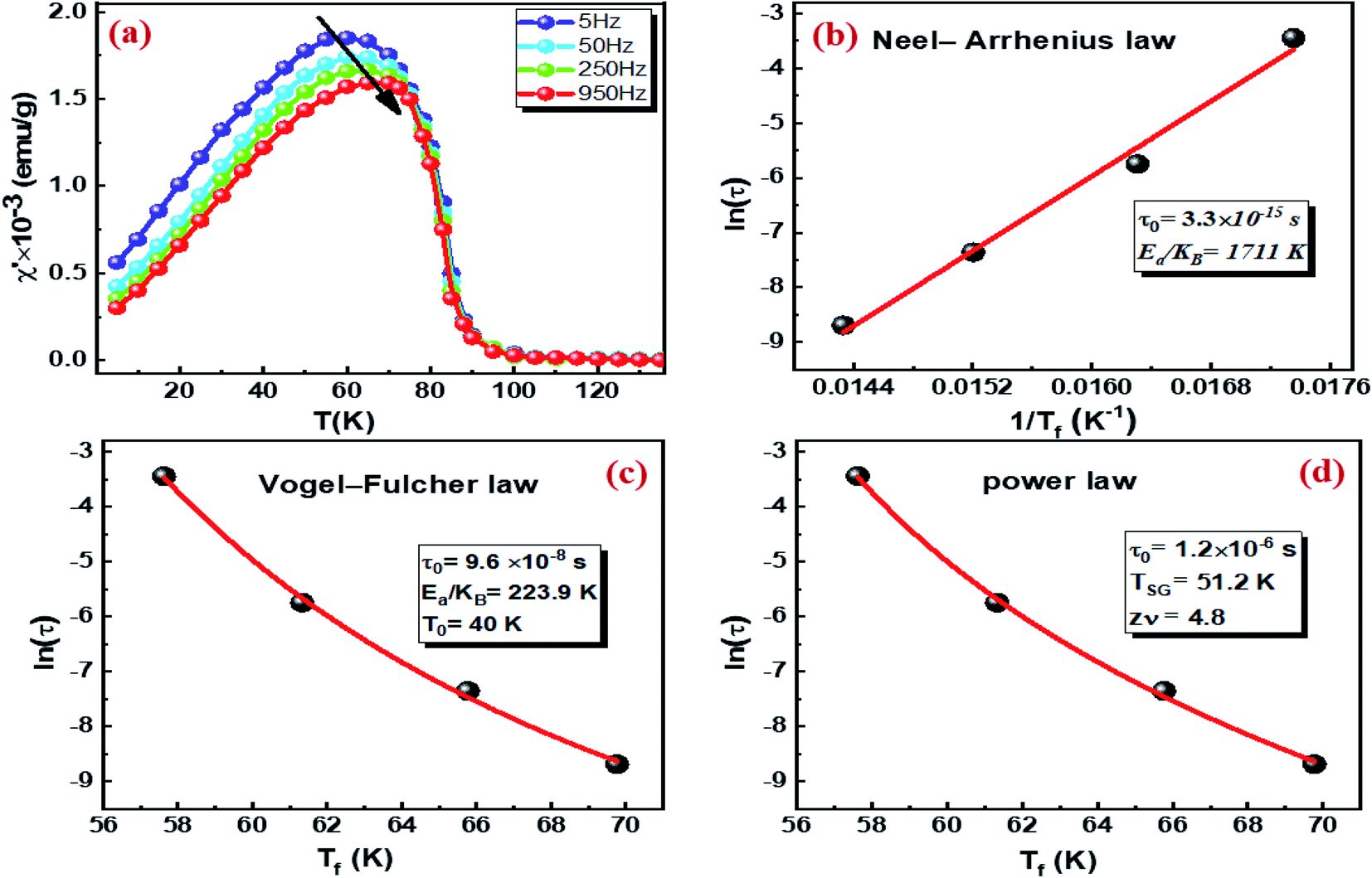 | ||
| Fig. 2 Temperature dependence of magnetic susceptibility (χ′) at different frequencies with an a.c. field of 10 Oe (a). The best fit of the relaxation times (τ) to the Neel–Arrhenius law (b) the Vogel–Fulcher law (c) and the power law (d) for the nanoparticles Cu1.5Mn1.5O4. | ||
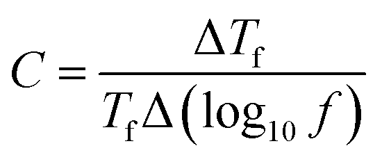
We first calculated the phenomenological parameter C (Mydosh parameter), representing the relative shift of the peak position with respect to the frequency, being a new indicator to distinguish the observed spin dynamic process53 as per the following equation:
 | (5) |
Generally, for spin glass and interacting particle systems C is located between 0.005 and 0.08,54 for clustered glass, C is about 0.03–0.08,54 for non-interacting superparamagnetism (SPM) C is between 0.1–0.13.54 In the present case, it is found that C is equal to 0.08, which supports spin-glass and/or cluster glass freezing. Hence, the superparamagnetism is blocked.
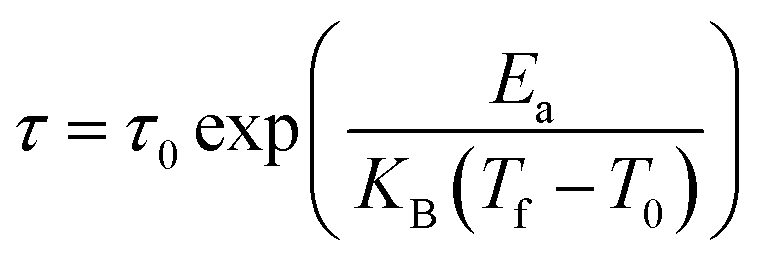
In order to verify the interaction between clusters and their influence on the fluctuation dynamics, different phenomenological models such as Neel–Arrhenius, Vogel–Fulcher and power law are examined. For non-interacting isolated SPM compound, we try to fit the experimental data of the relaxation time (τ) vs. freezing temperature (Tf) by the Néel–Arrhenius law without any critical behavior:55
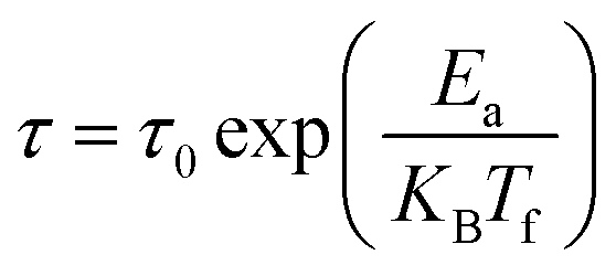 | (6) |
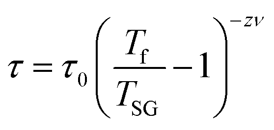
Accordingly, the relaxation behavior in the Cu1.5Mn1.5O4 compound is described either by spin glass or cluster glass. The relaxation behavior in Cu1.5Mn1.5O4 compound is described either by spin glass (SG) or by cluster glass (medium interaction). To further distinguish the state of relaxation behavior of copper manganite sample, we used Vogel–Fulcher's law, with an additional term T0 to deal with the interaction between clusters:55
 | (7) |
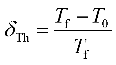
On the other hand, the parameter proposed by Tholence δTh related to the Vogel–Fulcher method is generally used to identify the type of spin interaction:55
 | (8) |
Generally, δTh is equal to 1 for the non-interacting particles (SPM). For the cluster glass system (weak interaction regime), the value of δTh must range between 0.3–0.6, while for spin-glass (SG) system (the medium to strong interaction regime), it's within 0.07–0.3.56 The δTh values obtained at different frequencies (see Table 2), characterize a weak interaction mechanism between the magnetic entities. This implies the existence of cluster glass state in the Cu1.5Mn1.5O4 sample.
| f (Hz) | δTh |
|---|---|
| 5 | 0.31 |
| 50 | 0.34 |
| 250 | 0.39 |
| 950 | 0.42 |
Finally, the critical spin dynamics, described by the conventional power law model, was exploited to eliminate the possibility of the spin glass behavior in the particle:55
 | (9) |
Fig. 3a presents isothermal magnetization curves recorded in the temperature range of 22–122 K in a magnetic field up to 5 T with temperature step 3 K. Below TC, the magnetization M increases rapidly and reaches saturation for low applied field values (0.5 T). This rapid increase corresponds to a rapid rearrangement of the Weiss domains in the direction of the applied magnetic field. This confirms a characteristic of FIM materials.34 Above TC, a decrease of M(μ0H) is observed with an almost linear behavior, which is typical for PM materials.34 Fig. 3b demonstrates the Arrott plots (H/M vs. M2) for Cu1.5Mn1.5O4 which are derived from the isothermal magnetizations. All curves in the Arrott graph show nonlinear behaviors, even in the high field region, indicating that critical behavior of Cu1.5Mn1.5O4 cannot be described by the conventional Stoner model. All the H/M vs. M2 curves show a positive slope. According to the criteria proposed by Banerjee,60 it suggests the occurrence of second-order magnetic transition. However, the non-linearity of the H/M vs. M2 indicates that the classical Arrott graph is invalid for Cu1.5Mn1.5O4.
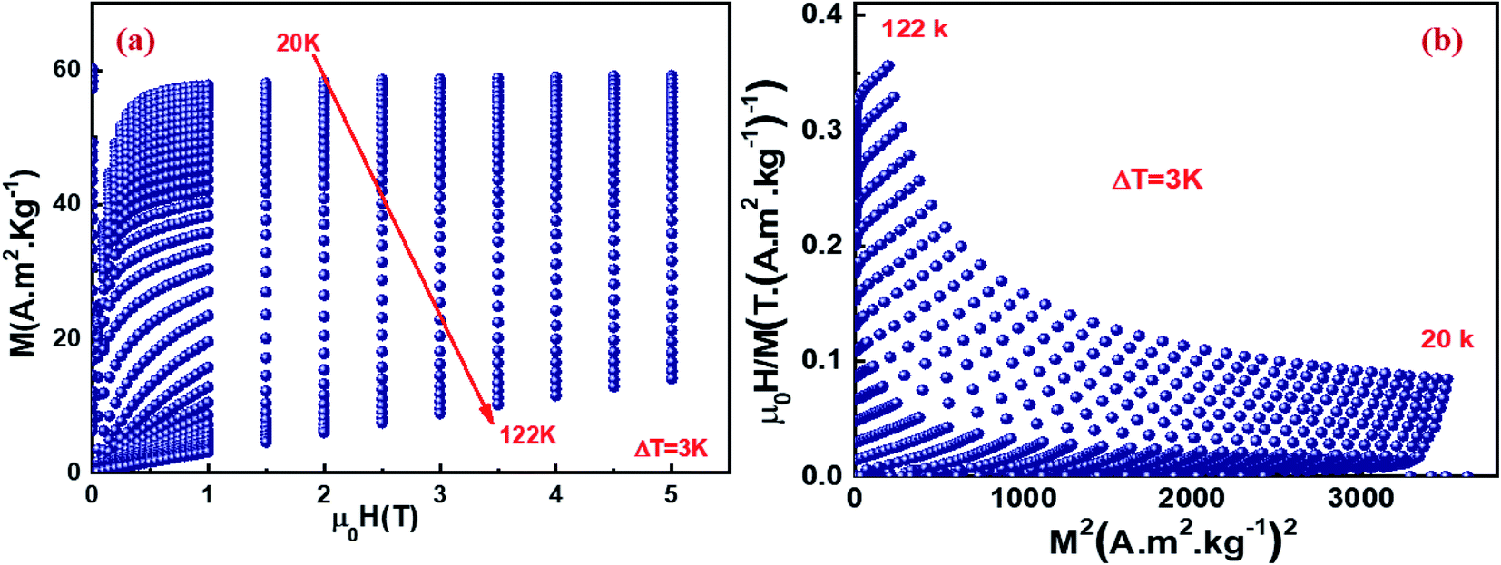 | ||
| Fig. 3 Isothermal magnetization curves for Cu1.5Mn1.5O4 nanoparticles measured at different temperatures around TC. (a). Arrott plot (μ0H/M vs. M2) isotherms (b). | ||
3.3 Magnetocaloric properties
In order to better elucidate the utility of our compound in magnetic refrigeration systems, the magnetic entropy change (ΔSM) induced indirectly from the isothermal magnetization curves, can be calculated using the approximated Maxwell equation.61 Therefore, the variation of the magnetic entropy can be computed numerically based on this equation:62
 | (10) |
Fig. 4a illustrates the temperature dependence of the magnetic entropy change (−ΔSM(T)) under different magnetic fields for Cu1.5Mn1.5O4 compound. The magnitude of −ΔSM increases as applied magnetic field increases and reached a maximum of 1.54, 2.52, 3.3, 3.97 and 4.58 J kg−1 K−1, distribute around the Curie temperature TC, for an applied magnetic field of 1, 2, 3, 4 and 5 T, respectively. To evaluate the cooling efficiency of our sample in the magnetic refrigeration field, we should calculate the relative cooling power (RCP)63 corresponding to the quantity of the heat transfer between the cold and hot sinks in the ideal refrigeration cycle, expressed as:
| RCP = −ΔSmaxM × δTFWHM | (11) |
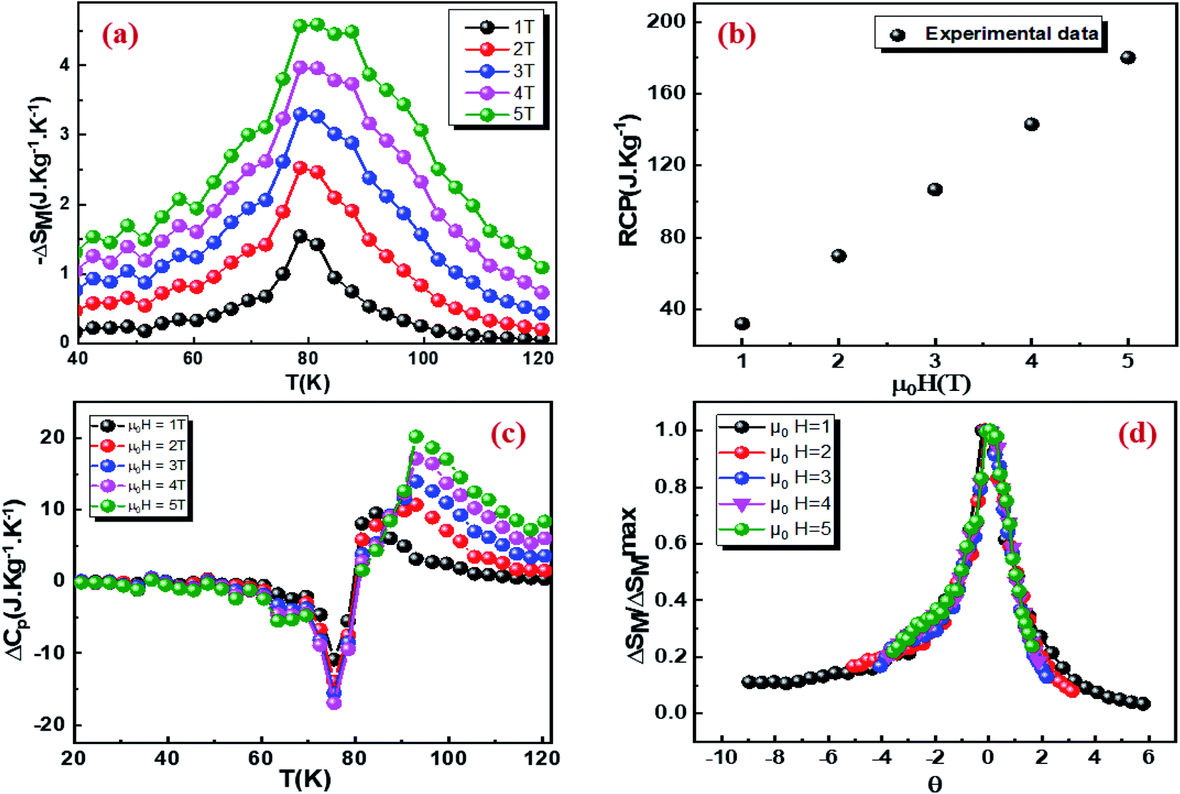 | ||
| Fig. 4 Temperature dependence of the magnetic entropy change (−ΔSM) under applied fields ranging from 1 to 5 T (a). Variation of (RCP) as a function of (μ0H) (b). Specific heat change (ΔCp) as a function of temperature at different applied magnetic fields (c) and normalized entropy change (ΔSM/ΔSmaxM) as a function of rescaled temperature (θ) for Cu1.5Mn1.5O4 nanoparticles (d). | ||
The RCP dependence of temperature at under different applied magnetic fields is displayed in Fig. 4b. It should be noted that gadolinium (Gd) is the best material that can be used in magnetic refrigeration at room temperature.64 The obtained values of (−ΔSmaxM) and (RCP) for our compound Cu1.5Mn1.5O4 are compared with the Gd as a reference and other magnetic spinel under 4 and 5 T presented in Table 3. The (−ΔSmaxM) and (RCP) values correspond to about 48.21 and 44% of those observed in pure Gd at 5 T. It is worth noting that the (RCP) value is high.34,65 Thus, our compound can be considered as active magnetic refrigerants.
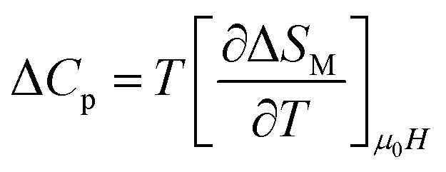
Fig. 4c displays the predicted results of the specific heat change (ΔCp) versus temperature under different field calculated by using the following formula:
 | (12) |
The (ΔCp) presents a negative value below TC and a positive one above TC that can strongly modify the total specific heat, which affects the heating or cooling power of the magnetic refrigerator.66
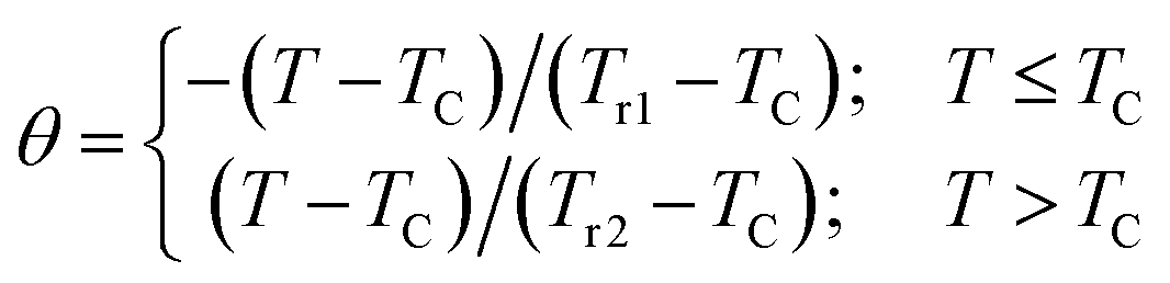
To further investigate the order of the magnetic phase transition in the sample, Franco et al.67 have suggested a phenomenological universal curve of the temperature dependence of the magnetic entropy ΔSM measured for different fields. Their suggestion is based on the assumption that, in the case of a second-order phase transition, all curves of the variation of magnetic entropy measured under different applied magnetic fields should collapse into one single new universal curve. While, in the case of a first order phase transition, the scaled curves do not obey a universal behavior.68 The construction of the phenomenological universal curve was performed by normalizing all the magnetic entropy change curves ΔSM with respect to their peak ΔSmaxM (ΔSM/ΔSmaxM) with the redimensioning of the temperature axis using two additional reference temperatures in a different way below and above TC as follows:69
 | (13) |
Fig. 4d unveils the universal curves of the magnetic entropy change of the Cu1.5Mn1.5O4 compound measured for the applied fields ranging from 1 up to 5 T. It is evident that all the normalized entropy change curves are reduced to a single curve, verifying the second-order FIM-PM phase transition for our material and displaying, therefore, a good agreement between Banerjee criterion and the Franco approximation.
Concerning the theoretical modeling of the magnetocaloric effect (MCE), Amaral et al. suggested a model based on the Landau theory of phase transition that takes into account the interaction between electrons and the magnetoelastic coupling effects in manganites.70,71 The magnetic energy M(μ0H) has been included in the expression of the Gibb's free energy.72 Based on the equilibrium condition at the Curie temperature, the obtained relation between the magnetization and the applied field can be written as:
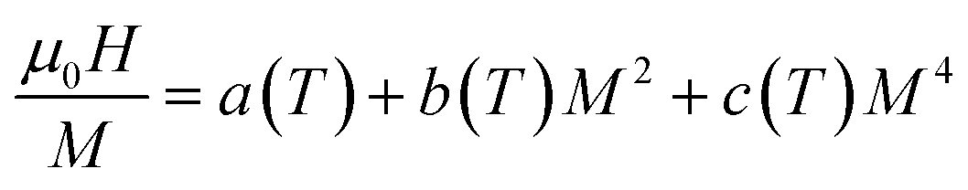 | (14) |
Landau's parameters a(T), b(T) and c(T) and their dependence on temperature determined from a polynomial fit of the experimental isothermal magnetizations (μ0H/M vs. M2) as illustrated in the inset (Fig. 5). We can notice that a(T) is always positive70,73 with a minimum at the Curie temperature TC corresponding to a maximum of the susceptibility, the sign of the Landau coefficient b(T) indicates the order of magnetic phase transition and includes the magnetoelastic and elastic contributions, b(TC) can be negative, zero, or positive. If b(TC) is negative, the transition is a first order; otherwise, it is a second order. Therefore, the magnetic transition in our compound Cu1.5Mn1.5O4 seems a second order. The magnetic entropy change is theoretically obtained by applying the differentiation of the free energy with respect to temperature, which has been given by the following equation:74
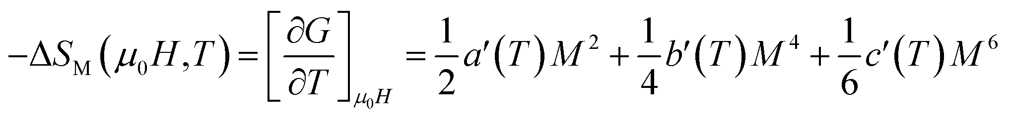 | (15) |
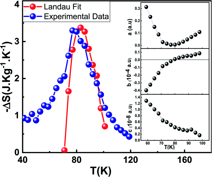 | ||
| Fig. 5 Experimental and theoretical magnetic entropy changes for Cu1.5Mn1.5O4 nanoparticles under 3 T applied magnetic field, the insets display the temperature dependence on Landau's coefficients a(T), b(T) and c(T). | ||
Fig. 5 exhibits a comparison between the magnetic entropy behavior obtained from the Maxwell relation integration of the experimental data from a magnetic field μ0H = 3 T and that calculated using Landau's theory. The theoretical and experimental curve of our sample shows some difference, especially below TC. Furthermore, the observed deviation of theoretically calculated ΔS from experimental results can be ascribed to magnetic disorder in the majority FIM phase. The existence of magnetic disorder inside the structure increases magnetization values for high-field values due to the unsaturated behavior of M(μ0H) isotherms, resulting in small shifts of Landau coefficients.75 These shifts will certainly affect theoretical ΔS values below TC. In our case, we are mainly interested in the use of the Landau theory to determine the maximum value of the exchange magnetic entropy and of TC, to compare them with the experimental. A good agreement is found between the experimental magnetic entropy change and the theoretical one in the vicinity of TC, which proves that both electron interaction and magnetoelastic coupling can account for the MCE properties,70,76 and determine the phase transition of this sample without taking into consideration either the Jahn–Teller distortion or exchange interaction.60
We determined the spontaneous magnetization (MS) in our Cu1.5Mn1.5O4 compound from the magnetic entropy ΔSM:77–79
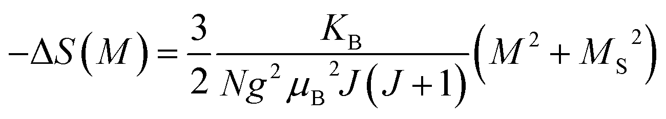 | (16) |
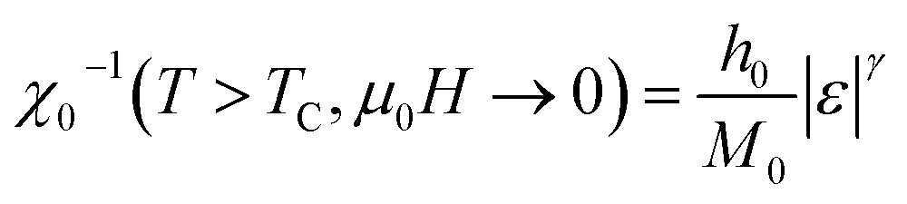
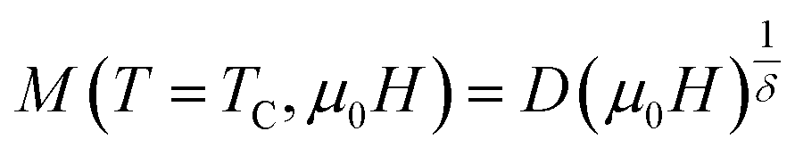
According to eqn (16), the plot of the isotherms (−ΔSM) vs. M2 is depicted in Fig. 6a. All the experimental data exhibit a linear variation. By fitting the (−ΔSM) vs. M2 data for T < TC, the value of MS can be calculated through the intersection of the straight lines with the M2 axis. For T > TC, the (−ΔSM) vs. M2 curves start at a null M value. On the other side, the linear fit applied in the linear regions of (H/M) vs. M2 allows us to determine the values of MS vs. T in Fig. 6b. Fig. 6c displays the spontaneous magnetization (MS) as a function of temperature. We notice that the temperature decreases as, the spontaneous magnetization increases, indicating that the system is approaching a spin ordering state at lower temperature. A good agreement was noticed in the behavior of MS vs. T estimated from (−ΔSM) vs. M2 curves (blue symbols) and the μ0H/M vs. M2 Arrott curves (red symbols). This confirms the validity of the change in magnetic entropy to determine the spontaneous magnetization values MS(T) of the Cu1.5Mn1.5O4 compound.
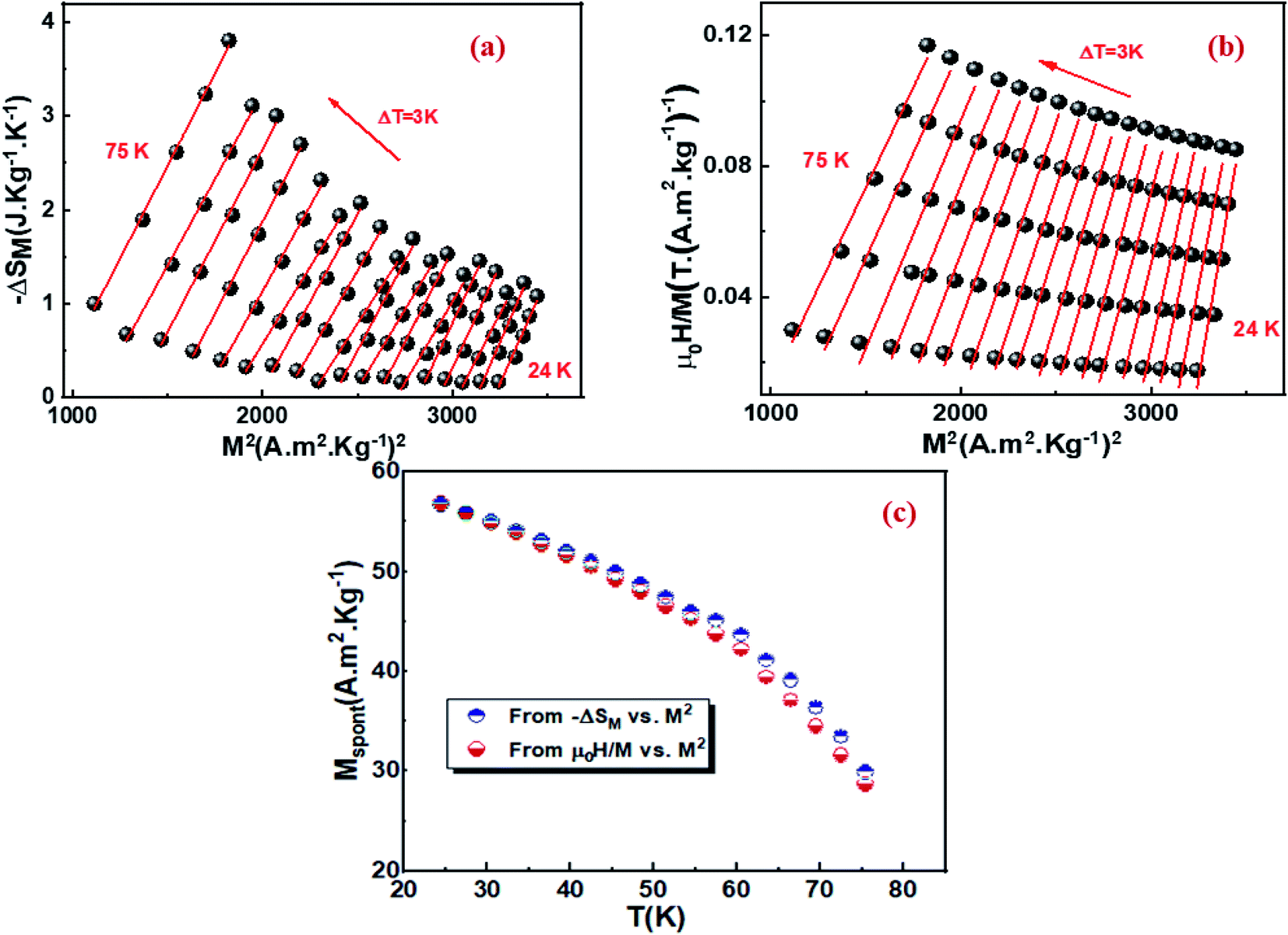 | ||
| Fig. 6 Isothermal (−ΔSM vs. M2) curves (a). Arrott plots (μ0H/M vs. M2) (b). Spontaneous magnetization of Cu1.5Mn1.5O4 nanoparticle, deduced from the extrapolation of the isothermal (−ΔSM vs. M2) curves and from the Arrott plots (μ0H/M vs. M2) (c). | ||
3.4 Critical behavior study
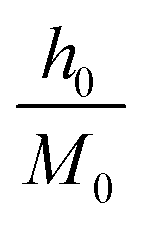
In accordance with the scaling hypothesis, a second-order magnetic material, near the Curie temperature TC, is characterized by a set of critical exponent β, γ, and δ,80 for instance, are associated with the spontaneous magnetization MS below TC, the magnetic susceptibility χ0−1 above TC and the critical magnetization isotherm at M(H, T = TC), respectively. The magnetization measurements are linked to these exponents as per the following asymptotic relations:81,82| MS(T < TC, μ0H → 0) = M0|ε|β | (17) |
 | (18) |
 | (19) |
 and D refer to the critical amplitudes.
In order to determine the Curie temperature TC as well as the critical exponents, various methods were used, such as the modified Arrott plot method “MAP”, the Kouvel–Fisher method “KF” and the critical isotherm analysis “CIA”. In the present study, to determine the most adequate model leading to correct exponents and a set of reasonably good parallel straight lines. Data analysis was carried out using a modified Arrott-plot “MAP” expression.83
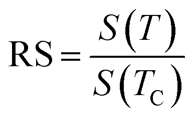
Fig. 7a–d demonstrates the modified Arrott plots (MAP) at different temperatures of the Cu1.5Mn1.5O4 compound obtained through diverse models: the mean-field model (β = 0.5, γ = 1 and δ = 3), the 3D Heisenberg model (β = 0.365, γ = 1.336 and δ = 4.80), the 3D Ising model (β = 0.325, γ = 1.240 and δ = 4.82) and the tri-critical mean field model (β = 0.25, γ = 1 and δ = 5). We observe at high fields, quasi-straight and nearly parallel lines, that seems difficult to differentiate the satisfactory model explaining the magnetic behavior for our compound.
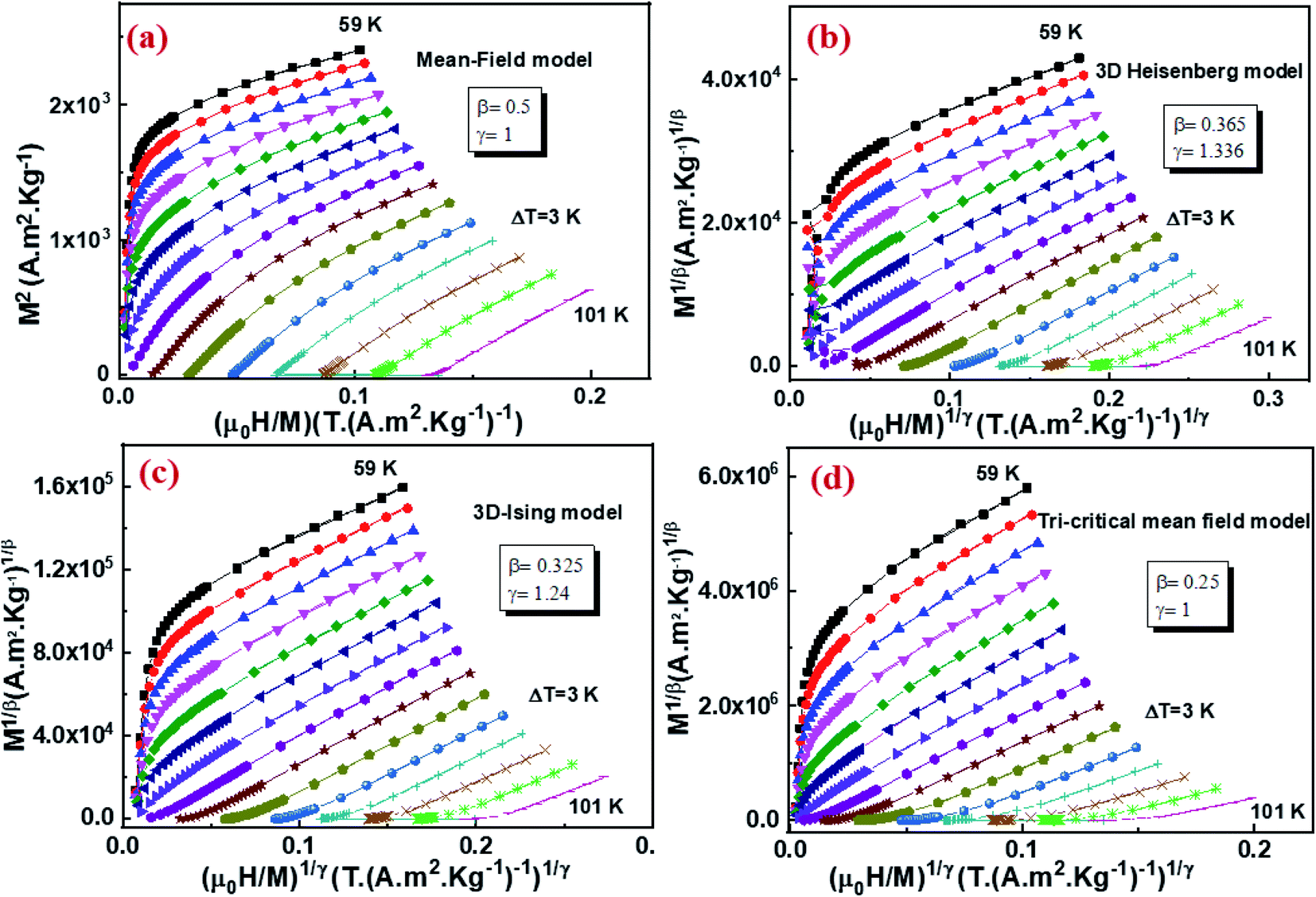 | ||
Fig. 7 Modified Arrott plots isotherms (MAP) 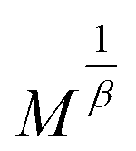 versus versus 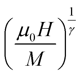 for Cu1.5Mn1.5O4 nanoparticles, with mean-field model (β = 0.5, γ = 1) (a), 3D Heisenberg model (β = 0.365, γ = 1.336) (b), 3D Ising model (β = 0.325, γ = 1.240) (c) and tri-critical mean field model (β = 0.25, γ = 1) (d). for Cu1.5Mn1.5O4 nanoparticles, with mean-field model (β = 0.5, γ = 1) (a), 3D Heisenberg model (β = 0.365, γ = 1.336) (b), 3D Ising model (β = 0.325, γ = 1.240) (c) and tri-critical mean field model (β = 0.25, γ = 1) (d). | ||
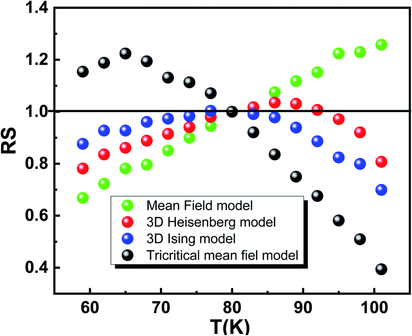
In that case we calculate the relative slope (RS), as a new indicator to identify the best model, from the following equation:
 | (20) |
The most satisfactory model is that which have an RS close to 1 (unit).82
Fig. 8 showcase the RS versus T curve of our compound for the four models. It can be observed that the 3D-Ising model is the most suitable model to describe the magnetic interactions inside Cu1.5Mn1.5O4 compound.
 | ||
| Fig. 8 Relative slope (RS) as a function of temperature for Cu1.5Mn1.5O4 nanoparticles. | ||
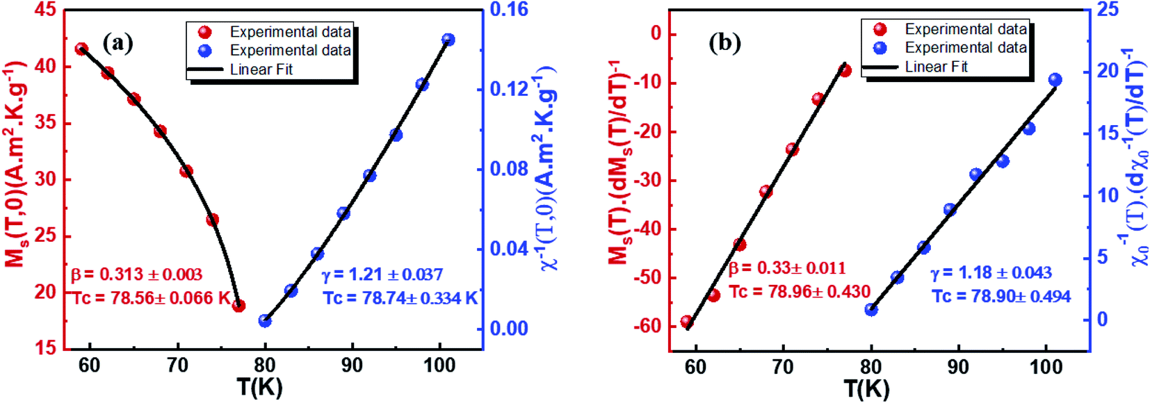
According to the “MAP”, the linear extrapolation of the curves at high field region of the isotherm makes to determine the values of the spontaneous magnetization (MS) and the inverse of the initial paramagnetic susceptibility (1/χ). The variations of MS(T) and χ−1(T) versus temperature are reported in Fig. 9a. The fitting of these plots as per eqn (17) and (18) gives us the values of the β and γ exponents as well as the value of TC (for details on the fits values, please see Table 3). We notice that the obtained critical exponents are very nearby to those associated with the best models obtained from RS curves.
 | ||
| Fig. 9 Temperature dependence of spontaneous magnetization MS(T) and inverse initial susceptibility χ0−1(T) along with fitting curves based on the power laws for Cu1.5Mn1.5O4 material (a). Kouvel–Fisher (KF) plot for the spontaneous magnetization MS(T) and the inverse susceptibility χ0−1(T), the solid lines are the linear fits of the data (b). | ||
A second method was exploited for more accurate determination of the critical exponent and TC value, known as Kouvel–Fisher “KF” method.84 This procedure is based on the following expressions:
 | (21) |
 | (22) |
Referring to eqn (21) and (22), we have plotted 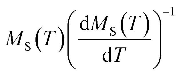 and
and 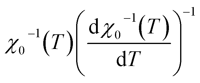 versus temperature. The plots follow a linear behavior with the slopes 1/β and 1/γ, respectively, and the intersections on the temperature axis give the values of TC.84
The KF plot has been presented in Fig. 9b. The values of the critical exponents as well as the Curie temperature are gathered in Table 4. We can notice that the obtained values of β and γ exponents as well as that of TC, calculated using both procedures, are consistent with each other. This suggests that the Arrott–Noakes and KF method are both feasible and effective to study the critical properties.
| Model/sample | Technique | TC (K) | β | γ | δ | Ref. |
|---|---|---|---|---|---|---|
| a CI – critical isotherm, exp. – experimental, cal. – calculated and MAP – modified Arrott plots. | ||||||
| Mean field model | Theory | 0.5 | 1 | 3 | 31 | |
| 3D Heisenberg model | Theory | 0.365 | 1.336 | 4.80 | 31 | |
| 3D Ising model | Theory | 0.325 | 1.240 | 4.82 | 31 | |
| Tri-critical mean field model | Theory | 0.25 | 1 | 5 | 31 | |
| Cu1.5Mn1.5O4 | MAP | 78.65 ± 0.4 | 0.313 ± 0.003 | 1.21 ± 0.037 | This work | |
| KF | 78.93 ± 0.462 | 0.33 ± 0.011 | 1.18 ± 0.043 | This work | ||
| CIA(exp.) | 4.54 ± 0.002 | This work | ||||
| CIA(cal.) | 4.86 | This work | ||||
Fig. 10 presents the critical isotherm curve M(H) at TC = 80 K. Using eqn (19), we can determine the third critical exponent δ from a linear adjustment of the M(H) at high field plotted on a log scale at the Curie temperature (see the inset of Fig. 10).
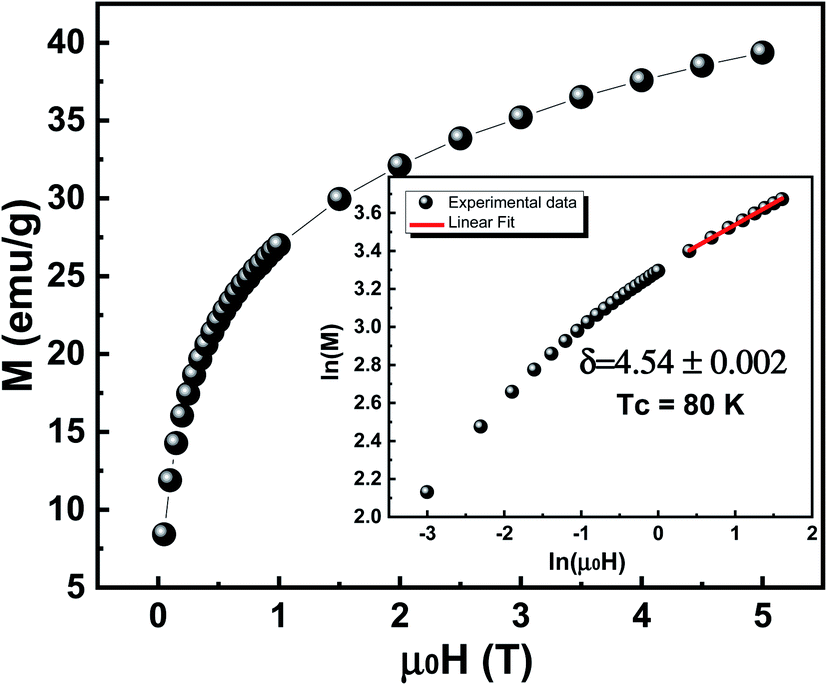 | ||
| Fig. 10 Critical isotherms of (M vs. μ0H) for Cu1.5Mn1.5O4 nanoparticles. The inset displays the same curve on log–log scale. | ||
The exponent δ can be also calculated from Widom scaling law given by:85
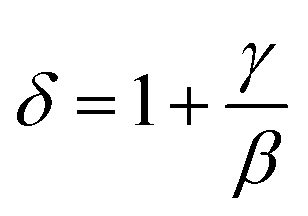 | (23) |
Using this expression, the δ value is 4.86. This value is comparable to that obtained by the magnetic isotherms at TC. The obtained values are summarized in Table 3. Consequently, these results ensure the reliability of the obtained β and γ values.
In order to test the reliability of the obtained critical exponent values, we have used the scaling hypothesis, assuming that both magnetization and internal magnetic field should obey the universal scaling law established by the following expression:86
 | (24) |
We have plotted in Fig. 11 the evolution of M |ε|−β as a function of μ0H |ε|−(β+γ) for the temperature range around TC, using values of β, γ and TC deduced from the “KF” method. By applying the logarithmic scale (in the inset of Fig. 11), we have carried out two independent branches, with the first one for temperature values below TC and the second one for temperature values above TC. As a result, these two universal curves confirm the agreement of the scaling hypothesis, suggesting the suitability of the obtained values of the critical exponents defining our model. The latter explains the magnetic interactions in compound.
 | ||
| Fig. 11 Scaling plots indicating two universal curves below and above TC for Cu1.5Mn1.5O4 nanoparticles. The inset presents the same curve on a log–log scale. | ||
4. Conclusion
In summary, the present research study examined the spin dynamics, the magnetic properties, the magnetocaloric effect and the critical behaviour near the magnetic phase transition temperature of Cu1.5Mn1.5O4 compound. The frequency-dependent ac susceptibility (χ′) data fitted with various phenomenological models such as the Neel–Arrhenius, Vogel–Fulcher and power law, suggests that the cluster glass state is formed in Cu1.5Mn1.5O4 sample. The magnetic measurements display a second order paramagnetic (PM)/ferrimagnetic (FIM) phase transition at Curie temperature. We have as well investigated the magnetocaloric effect MCE using Maxwell relation and Landau theory for Cu1.5Mn1.5O4. A good agreement was found between the experimental and theoretical calculations of (−ΔS) values of a magnetic field of 5 T, which reveals the importance of magnetoelastic coupling and electron interaction in the MCE properties of manganite systems. The relative cooling power (RCP) was predicted, which indicates that our material could be a good candidate for certain applications, including but not limited to refrigeration application. The magnetic entropy curves are found to follow the universal law, confirming the second-order ferrimagnetic (FIM) to paramagnetic (PM) phase transition at TC for our material. Therefore, a good agreement has been shown between Banerjee criterion and the Franco approximation. The spontaneous magnetization values estimated from the magnetic entropy change ((−ΔSM) vs. M2) are in excellent agreement with those determined from the classical extrapolation of Arrott curves (H/M vs. M2). By analyzing the isothermal magnetization around the Curie temperature TC and using several techniques such as modified Arrott plot (MAP), Kouvel–Fisher (KF) method and critical isotherm analysis (CIA), the values of β, γ, δ and TC are estimated.The obtained results are coherent with the 3D-Ising model for Cu1.5Mn1.5O4 compound. In addition the reliability of the critical exponent values was confirmed by Widom law, as well as the scaling hypothesis.
Conflicts of interest
The authors declare that they have no known competing financial interests or personal relationships that could have appeared to influence the work reported in this paper.Acknowledgements
This work is supported by: The authors extend their appreciation to the Deputyship for Research & Innovation, Ministry of Education in Saudi Arabia for funding this work through the project number “375213500”. The authors would like to extend their sincere appreciation to the central laboratory at Jouf University for supporting this study. The Tunisian National Ministry of Higher Education, Scientific Research and Technology.References
- P. N. Lisboa-Filho, M. Bahout, P. Barahona, C. Moure and O. Peña, J. Phys. Chem. Solids, 2005, 66, 1206–1212 CrossRef CAS.
- G. Pilania, V. Kocevski, J. A. Valdez, C. R. Kreller and B. P. Uberuaga, Commun. Mater., 2020, 1, 84 CrossRef.
- J. L. Dormann and M. Nogues, J. Phys. Condens. Matter, 1990, 2, 1223 CrossRef CAS.
- T. Tsutaoka, J. Appl. Phys., 2003, 93, 2789–2796 CrossRef CAS.
- J. Massoudi, M. Smari, K. Nouri, E. Dhahri, K. Khirouni, S. Bertaina and L. Bessais, RSC Adv., 2020, 10, 34556–34580 RSC.
- A. Bougoffa, J. Massoudi, M. Smari, E. Dhahri, K. Khirouni and L. Bessais, J. Mater. Sci.: Mater. Electron., 2019, 30, 21018–21031 CrossRef CAS.
- R. Peelamedu, C. Grimes, D. Agrawal, R. Roy and P. Yadoji, J. Mater. Res., 2003, 18, 2292–2295 CrossRef CAS.
- A. K. M. Akther Hossain, M. Seki, T. Kawai and H. Tabata, J. Appl. Phys., 2004, 96, 1273–1275 CrossRef CAS.
- S. Nayak, S. Thota, D. C. Joshi, M. Krautz, A. Waske, A. Behler, J. Eckert, T. Sarkar, M. S. Andersson and R. Mathieu, Phys. Rev. B, 2015, 92, 214434 CrossRef.
- W. Yang, X. Kan, X. Liu, Z. Wang, Z. Chen, Z. Wang, R. Zhu and M. Shezad, Ceram. Int., 2019, 45, 23328–23332 CrossRef CAS.
- Y. Moritomo, Y. Tomioka, A. Asamitsu, Y. Tokura and Y. Matsui, Phys. Rev. B: Condens. Matter Mater. Phys., 1995, 51, 3297 CrossRef CAS PubMed.
- J. A. Mydosh, J. Magn. Magn. Mater., 1996, 157, 606–610 CrossRef.
- S. Karmakar, S. Taran, E. Bose, B. K. Chaudhuri, C. P. Sun, C. L. Huang and H. D. Yang, Phys. Rev. B: Condens. Matter Mater. Phys., 2008, 77, 144409 CrossRef.
- S. Kirkpatrick and D. Sherrington, Phys. Rev. B: Condens. Matter Mater. Phys., 1978, 17, 4384 CrossRef CAS.
- R. D. McMichael, R. D. Shull, L. J. Swartzendruber, L. H. Bennett and R. E. Watson, J. Magn. Magn. Mater., 1992, 111, 29–33 CrossRef CAS.
- M. Zborowski, in Physics of Magnetic Cell Sorting Scientific and Clinical Applications of Magnetic Carriers, ed. M. Zborowski, Plenum, New York, 1997 Search PubMed.
- D. G. Mitchell, J. Magn. Reson. Imaging, 1997, 7, 1–4 CrossRef CAS PubMed.
- K. Raj, B. Moskowitz and R. Casciari, J. Magn. Magn. Mater., 1995, 149, 174–180 CrossRef CAS.
- M. H. Kryder, MRS Bull., 1996, 21, 17–22 CrossRef.
- V. V. Gridin, G. R. Hearne and J. M. Honig, Phys. Rev. B: Condens. Matter Mater. Phys., 1996, 53, 15518 CrossRef CAS PubMed.
- J.-M. Li, A. C. H. Huan, L. Wang, Y.-W. Du and D. Feng, Phys. Rev. B: Condens. Matter Mater. Phys., 2000, 61, 6876 CrossRef CAS.
- R. H. Kodama, A. E. Berkowitz, E. J. McNiff, Jr and S. Foner, Phys. Rev. Lett., 1996, 77, 394 CrossRef CAS PubMed.
- M. F. Jönsson, Phys. Rev. B: Condens. Matter Mater. Phys., 2000, 61, 1261 CrossRef.
- D. Peddis, D. Rinaldi, G. Ennas, A. Scano, E. Agostinelli and D. Fiorani, Phys. Chem. Chem. Phys., 2012, 14, 3162–3169 RSC.
- C. Tien, C. H. Feng, C. S. Wur and J. J. Lu, Phys. Rev. B: Condens. Matter Mater. Phys., 2000, 61, 12151 CrossRef CAS.
- J. A. Mydosh, Spin glasses: an experimental introduction, Taylor and Francis, 1993 Search PubMed.
- H. Szymczak, M. Baran, G.-J. Babonas, R. Diduszko, J. Fink-Finowicki and R. Szymczak, J. Magn. Magn. Mater., 2005, 285, 386–394 CrossRef CAS.
- K. Anil and P. A. Joy, J. Phys. Condens. Matter, 1998, 10, L487–L493 CrossRef.
- J. L. Alonso, L. A. Fernández, F. Guinea, V. Laliena and V. Martín-Mayor, Nucl. Phys. B, 2001, 596, 587–610 CrossRef.
- A. K. Pramanik and A. Banerjee, Phys. Rev. B: Condens. Matter Mater. Phys., 2009, 79, 214426 CrossRef.
- H. E. Stanley, Introduction to Phase Transitions and Critical Phenomena, Oxford University Press, Oxford, 1971 Search PubMed.
- S. N. Kaul, J. Magn. Magn. Mater., 1985, 53, 5–53 CrossRef CAS.
- A. Waskowska, L. Gerward, J. S. Olsen, S. Steenstrup and E. Talik, J. Phys. Condens. Matter, 2001, 13, 2549 CrossRef CAS.
- K. Vinod, A. T. Satya, N. R. Ravindran and A. Mani, Mater. Res. Express, 2018, 5, 056104 CrossRef.
- S. Mohanta, S. D. Kaushik and I. Naik, Solid State Commun., 2019, 287, 94–98 CrossRef CAS.
- H. Zhao, X. X. Zhou, L. Y. Pan, M. Wang, H. R. Chen and J. L. Shi, RSC Adv., 2017, 7, 20451–20459 RSC.
- J. Quan, L. Mei, Z. Ma, J. Huang and D. Li, RSC Adv., 2016, 6, 55786–55791 RSC.
- R. E. Vandenberghe, G. G. Robbrecht and V. A. M. Brabers, Mater. Res. Bull., 1973, 8, 571–579 CrossRef CAS.
- A. Hadded, J. Massoudi, E. Dhahri, K. Khirouni and B. F. O. Costa, RSC Adv., 2020, 10, 42542–42556 RSC.
- A. Mabrouki, T. Mnasri, A. Bougoffa, A. Benali, E. Dhahri and M. A. Valente, J. Alloys Compd., 2021, 860, 157922 CrossRef CAS.
- J. A. Mydosh, Spin glasses: an experimental introduction, Taylor and Francis, 1993 Search PubMed.
- S. Mukherjee, R. Ranganathan, P. S. Anilkumar and P. A. Joy, Phys. Rev. B: Condens. Matter Mater. Phys., 1996, 54, 9267 CrossRef CAS PubMed.
- I. G. Deac, J. F. Mitchell and P. Schiffer, Phys. Rev. B: Condens. Matter Mater. Phys., 2001, 63, 172408 CrossRef.
- S. G. Yang, T. Li, B. X. Gu, Y. W. Du, H. Y. Sung, S. T. Hung, C. Y. Wong and A. B. Pakhomov, Appl. Phys. Lett., 2003, 83, 3746–3748 CrossRef CAS.
- D. P. Shoemaker, J. Li and R. Seshadri, J. Am. Chem. Soc., 2009, 131, 11450–11457 CrossRef CAS PubMed.
- P. Patra, I. Naik, S. D. Kaushik, S. Mukherjee and S. Mohanta, 2020, arXiv preprint arXiv:2008.04571.
- G. M. Al-Senani, O. H. Abd-Elkader and N. M. Deraz, Appl, 2021, 11, 2034 Search PubMed.
- A. Tozri, J. Khelifi, E. Dhahri and E. K. Hlil, Mater. Chem. Phys., 2015, 149, 728–733 CrossRef.
- M. Khlifi, M. Wali and E. Dhahri, Phys. B, 2014, 449, 36–41 CrossRef CAS.
- S. Åsbrink, A. Waśkowska and E. Talik, J. Phys. Chem. Solids, 1999, 60, 573–577 CrossRef.
- D. Gangwar and C. Rath, Phys. Chem. Chem. Phys., 2020, 22, 14236–14245 RSC.
- A. Tokarev, P. Agulhon, J. Long, F. Quignard, M. Robitzer, R. A. Ferreira, L. D. Carlos, J. Larionova, C. Guérin and Y. Guari, J. Mater. Chem., 2012, 22, 20232–20242 RSC.
- M. K. Singh, W. Prellier, M. P. Singh, R. S. Katiyar and J. F. Scott, Phys. Rev. B: Condens. Matter Mater. Phys., 2008, 77, 144403 CrossRef.
- D. Gangwar and C. Rath, Phys. Chem. Chem. Phys., 2020, 22, 14236–14245 RSC.
- J. Massoudi, M. Smari, K. Khirouni, E. Dhahri and L. Bessais, J. Magn. Magn. Mater., 2021, 528, 167806 CrossRef.
- D. M. Neacsa, G. Gruener, S. Hebert and J.-C. Soret, J. Magn. Magn. Mater., 2017, 432, 68–76 CrossRef CAS.
- J. Souletie and J. L. Tholence, Phys. Rev. B: Condens. Matter Mater. Phys., 1985, 32, 516 CrossRef CAS PubMed.
- S. Akhter, D. P. Paul, S. M. Hoque, M. A. Hakim, M. Hudl, R. Mathieu and P. Nordblad, J. Magn. Magn. Mater., 2014, 367, 75–80 CrossRef CAS.
- D. Soukup, S. Moise, E. Céspedes, J. Dobson and N. D. Telling, ACS Nano, 2015, 9, 231–240 CrossRef CAS PubMed.
- K. Dey, A. Indra, S. Majumdar and S. Giri, J. Magn. Magn. Mater., 2017, 435, 15–20 CrossRef CAS.
- R. Skini, A. Omri, M. Khlifi, E. Dhahri and E. K. Hlil, J. Magn. Magn. Mater., 2014, 364, 5–10 CrossRef CAS.
- A. Mabrouki, A. Benali, T. Mnasri, E. Dhahri, M. A. Valente and M. Jemmali, J. Mater. Sci.: Mater. Electron., 2020, 31, 22749–22767 CrossRef CAS.
- M. Jeddi, H. Gharsallah, M. Bejar, M. Bekri, E. Dhahri and E. K. Hlil, RSC Adv., 2018, 8, 9430–9439 RSC.
- V. K. Pecharsky and K. A. Gschneidner, Jr, Phys. Rev. Lett., 1997, 78, 4494–4497 CrossRef CAS.
- S. Bahhar, A. Boutahar, L. H. Omari, H. Lemziouka, E. K. Hlil and H. Bioud, Solid State Commun., 2020, 322, 114056 CrossRef CAS.
- M. Jeddi, H. Gharsallah, M. Bekri, E. Dhahri and E. K. Hlil, J. Mater. Sci.: Mater. Electron., 2019, 30, 14430–14444 CrossRef CAS.
- V. Franco, A. Conde, J. M. Romero-Enrique and J. S. Blázquez, J. Phys. Condens. Matter, 2008, 20, 285207 CrossRef.
- C. M. Bonilla, J. Herrero-Albillos, F. Bartolomé, L. M. García, M. Parra-Borderías and V. Franco, Phys. Rev. B: Condens. Matter Mater. Phys., 2010, 81, 224424 CrossRef.
- R. Tlili, A. Omri, M. Bejar, E. Dhahri and E. K. Hlil, Ceram. Int., 2015, 41, 10654–10658 CrossRef CAS.
- V. S. Amaral and J. S. Amaral, J. Magn. Magn. Mater., 2004, 272, 2104–2105 CrossRef.
- J. S. Amaral, M. S. Reis, V. S. Amaral, T. M. Mendonca, J. P. Araujo and M. A. Sa, J. Magn. Magn. Mater., 2005, 290, 686 CrossRef.
- J. S. Amaral and V. S. Amaral, J. Magn. Magn. Mater., 2010, 322, 1552–1557 CrossRef CAS.
- J. Inoue and M. Shimizu, Phys. Lett. A, 1982, 90, 85–88 CrossRef.
- M. S. Anwar, S. Kumar, F. Ahmed, N. Arshi, G. W. Kim and B. H. Koo, J. Korean Phys. Soc., 2012, 60, 1587–1592 CrossRef CAS.
- W. Mabrouki, A. Krichene, N. C. Boudjada and W. Boujelben, Appl. Phys. A, 2020, 126, 1–12 CrossRef.
- S. Chandra, A. Biswas, M.-H. Phan and H. Srikanth, J. Magn. Magn. Mater., 2015, 384, 138–143 CrossRef CAS.
- A. M. Tishin and Y. I. Spichkin, The magnetocaloric effect and its applications, CRC Press, 2016 Search PubMed.
- X. Si, Y. Shen, X. Ma, S. Chen, J. Lin, J. Yang, T. Gao and Y. Liu, Acta Mater., 2018, 143, 306–317 CrossRef CAS.
- J. C. Debnath, A. M. Strydom, P. Shamba, J. L. Wang and S. X. Dou, J. Appl. Phys., 2013, 113, 233903 CrossRef.
- H. E. Stanley, Introduction to Phase Transitions and Critical Phenomena, Oxford University Press, Oxford, 1971 Search PubMed.
- K. Huang, Introduction to statistical physics, New York, 1987, p. 263 Search PubMed.
- C. V. Mohan, M. Seeger, H. Kronmüller, P. Murugaraj and J. Maier, J. Magn. Magn. Mater., 1998, 183, 348–355 CrossRef CAS.
- A. Arrott and J. E. Noakes, Phys. Rev. Lett., 1967, 19, 786 CrossRef CAS.
- J. S. Kouvel and M. E. Fisher, Phys. Rev., 1964, 136, A1626 CrossRef.
- N. Assoudi, I. Walha, K. Nouri, E. Dhahri and L. Bessais, J. Alloys Compd., 2018, 753, 282–291 CrossRef CAS.
- J. Yang and Y. P. Lee, Appl. Phys. Lett., 2007, 91, 142512 CrossRef.
| This journal is © The Royal Society of Chemistry 2021 |