Application of hyperspectral imaging technology for rapid identification of Ruditapes philippinarum contaminated by heavy metals

Abstract

Human beings are confronted with a serious health hazard when ingesting Ruditapes philippinarum contaminated with heavy metals, and thus it is significantly necessary to identify heavy metal contaminated Ruditapes philippinarum. This study investigates the feasibility of hyperspectral imaging to identify heavy metal contamination in Ruditapes philippinarum rapidly. To reduce the effects of noise, four different spectral pretreatments were performed on the original spectra. To select characteristic wavebands for identification, four waveband selection algorithms based on neighbourhood rough set theory were proposed, namely, mutual information, consistency measure, dependency measure, and variable precision. The selected wavebands were input to an extreme learning machine to construct classification models. The results demonstrated that multiplicative scatter correction pretreatment was suitable for Ruditapes philippinarum hyperspectral imaging datasets. The identification models exhibited satisfactory performance to distinguish healthy Ruditapes philippinarum from those contaminated by both individual and multiple heavy metals. The identification results of Cd and Pb contaminated samples were more accurate than those of Cu and Zn contaminated samples. When the number of training samples decreased the identification performance decreased, but not significantly. The results showed that combined with pattern recognition analysis hyperspectral imaging technology can be used to distinguish healthy Ruditapes philippinarum samples from those contaminated by heavy metals, even with only a small number of training samples. This model is suitable for applications in analysing many shellfish rapidly and non-destructively.

---

1. Introduction

Shellfish, with high nutritive value, constitute an important part of global seafood consumption. In China, Ruditapes philippinarum is a widely consumed shellfish species. As a nutrient-rich food, it has high protein and unsaturated fatty acids, low cholesterol and fat, and various trace elements. Customers favour its freshness, good flavour, and low prices. Ruditapes philippinarum mainly grows in tidal areas close to coastlines or in estuaries, where it is at high risk of exposure to heavy metal contamination. It can quickly accumulate heavy metal concentrations because of its low mobility and non-selective filter-feeding behaviour.¹ Heavy metals such as copper (Cu), lead (Pb), cadmium (Cd), and zinc (Zn) contaminate the aquatic environment and pollute aquatic products.² With rapid accumulation of high concentrations of heavy metals, it poses a hazard to human health.³

At present, standard methods to detect heavy metals include flame atomic absorption spectrometry, graphite furnace atomic absorption spectrometry, and atomic fluorescence spectrometry,^4,5 which can precisely measure the types and concentrations of the heavy metals. However, these methods do not facilitate rapid food safety inspection because of their high cost, intensive labour needs, complex preparation requirements, and time-consuming nature.⁶ Thus, a fast, low-cost, and reliable method is required to detect heavy metal contamination.

Although the near-infrared spectroscopy (NIRS) technique facilitates a fast and low-cost qualitative or quantitative determination of heavy metal levels, and has been applied extensively in quality control, the technique requires sample pretreatment and the use of chemical reagents. The NIRS reflects the vibrations of chemical bonds at different wavelengths. When samples are illuminated by a spectrophotometer, different chemical bond types within the organisms absorb or emit light at different wavelengths.⁷ Although heavy metals usually display no infrared activity and almost no characteristic peaks, the NIRS technique can indirectly detect heavy metals. The heavy metals in contaminated Ruditapes philippinarum induce the synthesis of detoxification proteins and inhibit antioxidant enzymes. These effects modify the structures and concentrations of relevant biological molecules, and the molecular vibration information in the infrared spectrum is obtained from these changes.⁸ Therefore, it can be applied to detect heavy metals indirectly about the infrared spectral information acquired by the interactions between heavy metal ions and enzymes. With the development of spectral technology, hyperspectral imaging (HSI) combines spectral analysis with traditional computer imaging with the use of spatial and spectral information to create a three-dimensional dataset that contains numerous images of the sample at different wavelengths. Hence, HSI has the potential to become a powerful technique for food quality and safety evaluation.^9,10

HSI technology is suitable for quality control. Recently, it has been applied to agricultural products such as meat products, fruits, vegetables, dairy products, and cereals.^11,12 For aquatic products, the HSI technology has been used to evaluate the safety and quality of various products, including the detection of fish fillet substitution and mislabelling, automated sorting for size and sex of sea bass, and automatic evaluation of freshness of gilthead sea bream.^13,14 To date, few studies have investigated NIRS for the identification of heavy metal contaminated shellfish. Hu et al. used mid-infrared spectroscopy to estimate Cu content in Tegillarca granosa.³ Chen et al. applied an infrared spectroscopy approach to identify healthy Tegillarca granosa from samples contaminated by unspecified heavy metals.⁸ To identify contaminated Tegillarca granosa samples, competitive adaptive reweighted sampling methods, genetic algorithms, and successive projection algorithms had been used.⁴ In these studies, the samples were freeze-dried and ground into a powder prior to collecting the spectral. These studies indicate that NIRS is a feasible method for identification of heavy metal contaminated shellfish. However, there is little documented information on the use of HSI to identify heavy metal contaminated Ruditapes philippinarum, or shellfish more generally.

In this study, the HSI technology was developed to rapidly detect heavy metal contaminated Ruditapes philippinarum samples. Healthy Ruditapes philippinarum samples were manually contaminated by Zn, Cu, Cd, and Pb; then the ability of HSI technology to identify heavy metals was evaluated. To the best of our knowledge, this is the first study to identify Ruditapes philippinarum contaminated with heavy metals with the use of HSI technology and chemometrics. Compared with traditional laboratory-based techniques, the HSI technology neither requires chemical reagents nor pollutes the environment. In addition, it has been shown to improve efficiency by saving time, reducing labour needs, and removing the need for sample pretreatment.¹⁵

Unfortunately, noise in the sample information is unavoidable in the spectra obtained from the HSI technology. Thus, before the setup of the models, the spectra need to be pretreated to reduce noise and physical factors, such as particle size and path length. Additionally, in the HSI datasets, there is substantial irrelevant or redundant information. To increase the accuracy and the speed of the models, it is crucial to extract effective wavebands from the available range of wavebands.

The objectives of this study were to (1) investigate the effects of standard normal variate (SNV), multiplicative scatter correction (MSC), Savitzky–Golay smoothing (SG), and first derivative (DER) four different spectral pretreatments, and hence, identify the optimal pretreatment method; (2) extract characteristic wavebands that identify Ruditapes philippinarum samples contaminated with heavy metals with the application of the neighbourhood rough set (NRS) theory; (3) build extreme learning machine (ELM) classification models with selected wavebands to identify heavy metal contaminated Ruditapes philippinarum samples; (4) analyse the influence of neighbourhood size on the number of selected wavebands and classification accuracy; and (5) research the effect on identification results to reduce the number of training samples. The main aim of the study was to assess the HSI technique as a qualitative tool to rapidly detect heavy metal contamination in Ruditapes philippinarum, and improve the food safety.

2. Materials and methods

2.1 Sample preparation

Ruditapes philippinarum were purchased from the Cunjin Seafood Market in Zhanjiang, China in December 2019. Seawater was filtered over 24 h to remove sand, and then used for Ruditapes philippinarum cultivation. The seawater had pH of 8.0, water temperature of 28 °C, dissolved oxygen content of 6.5 mg L⁻¹, and salinity level of 30‰. Fine sand was sterilized, and any impurity was removed before being used to cover the bottom of five tanks. The cubic dimensions of the tanks were 119 × 108 × 32 cm, and each tank volume was 300 L. A constant volume of seawater and chemical reagents were added to each tank to simulate the polluted environment. Ruditapes philippinarum were exposed to high concentrations of Pb(CH₃COO)₂·3H₂O (0.9 mg L⁻¹), CuSO₄·5H₂O (0.05 mg L⁻¹), CdC1₂·2.5H₂O (0.8 mg L⁻¹), and ZnSO₄·7H₂O (2.2 mg L⁻¹) in the seawater tanks. The selection of heavy metal concentrations was based on the median lethal concentration (the concentration of the heavy metal that caused lethal effects in 50% of tested organisms) and was determined by raising experiments several times. A control group of Ruditapes philippinarum samples was raised in the identical seawater and tank, but without any heavy metals.

During the experiment, seawater was continuously aerated and filtered through an aquarium pump that was connected to a PVC box (55 × 10.2 × 46 cm) containing filtration materials. The Ruditapes philippinarum were fed daily with spirulina algae powder, and the filter was shut off for four hours during the feeding. Fresh seawater with heavy metals was added to the tanks to compensate for the pillage and evaporation. All Ruditapes philippinarum samples were reared for 10 d to allow heavy metal accumulation. Some Ruditapes philippinarum died during this period. Those exposed to Cd suffered the highest mortality, whereas those exposed to Zn suffered the lowest. After the rearing period, 60 contaminated samples per heavy metal tank (Cu, Cd, Pb, and Zn), and 120 healthy (uncontaminated) Ruditapes philippinarum samples were collected for spectral measurements.

2.2 HSI spectral acquisition and pretreatments

The HSI datasets for Ruditapes philippinarum samples were acquired with the use of a SOC710-VP hyperspectral imager (Surface Optics Corporation, San Diego, CA, USA) in the visible near-infrared range. The HSI system was composed of a SOC710-VP hyperspectral imager, a light source (halogen lamps), and a platform unit.¹⁶ The HSI system used in this study was shown in Fig. 1. The hyperspectral imager can record spectra at the 367.7–1051.9 nm range with 512 wavebands. The wavebands located near two extremes of the range contain with considerable noise were removed. The retained dataset thus became 450 wavebands from 400.5 nm to 1000.9 nm.

Fig. 1 The HSI system.

Ruditapes philippinarum were removed from the seawater tanks, dried with a towel and the shells were opened. An individual Ruditapes philippinarum, now in half of its shell, was placed on the platform. The HSI information of each sample was collected with the use of the HSI system and HyperScanner2.0 data acquisition software. To reduce external interference, the acquisition process was completed in a dark room. It was shown in Fig. 2 about the hyperspectral images for the Ruditapes philippinarum control group samples, and those contaminated with heavy metals (Cd, Cu, Pb, and Zn). With the SRAnal710 software, a standard calibration procedure was performed on the acquired hyperspectral images, including spectral calibration, radiometric calibration, and reflectance normalisation.

Fig. 2 Hyperspectral images of Ruditapes philippinarum samples (a) healthy samples, (b) samples contaminated by Cd, (c) samples contaminated by Cu, (d) samples contaminated by Pb, and (e) samples contaminated by Zn.

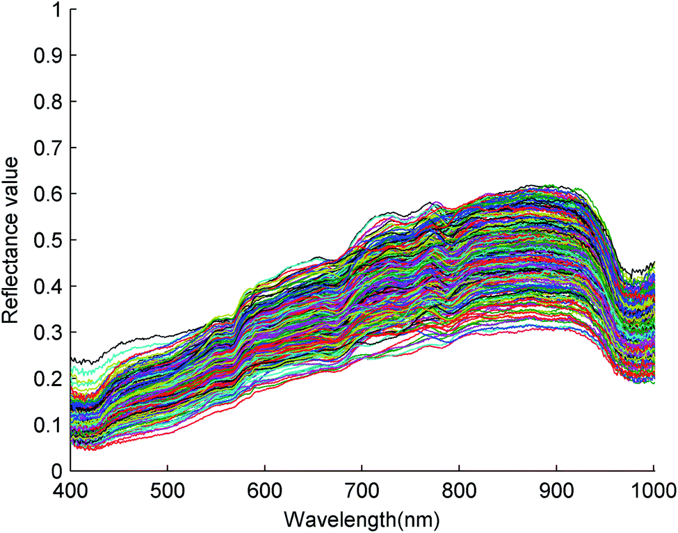
For hyperspectral images of Ruditapes philippinarum samples, the region of interest (ROI) was a rectangle area (1000 pixels) around the centre of a sample. The ROI area was controlled by ENVI 4.8 software (Research Systems Inc., USA). The pixel spectra within each ROI were extracted and averaged to represent the original sample spectrum. The spectra of all the Ruditapes philippinarum samples, from the five groups (healthy, contaminated by Zn, Cd, Pb, and Cu), were presented in Fig. 3. Because all five spectra were related to the same species, the spectra of samples were similar. To fully observe the differences in the spectra among the five groups of Ruditapes philippinarum, the average spectral curve of each group was shown in Fig. 4. Similar trends were observed in the average spectral curves; however, there were some differences in the spectral reflectance values.

Fig. 3 The spectra of all Ruditapes philippinarum samples.

Fig. 4 Average spectral curve of each group.

In the region of 700 to 1000 nm, samples contaminated by Cd had the lowest average spectral reflectance, followed by the healthy samples. The spectral curves of samples contaminated by Cu, Zn, and Pb serious overlapped and were above the spectra of the healthy samples and samples contaminated by Cd. However, in the region of 400 to 650 nm, the spectral reflectance of samples contaminated by Zn was lower than that of the healthy samples. The spectra of these biological samples were extremely complex due to the light absorption and scattering processes associated with their microstructure. It was difficult to identify the obvious visual differences in the spectra caused by heavy metal contamination. Therefore, to ensure the distinction among the data, chemometrics and pattern recognition methods were employed. In our study, different pretreatment methods were employed to accentuate the differences between samples and amplify changes in the spectra. Waveband selection methods of the NRS theory were utilized to solve the problem that it was difficult to select the useful wavebands, caused by the overlapping spectra.

The collected HSI data usually contained noise. Therefore, before the setup of classification models, the spectra were supposed to be pretreated and the noise was reduced. In this study, four pretreatment methods (MSC, SG, SNV, and DER) were applied. The SG was an effective tool to reduce the high-frequency noise component, and an SG method using the third-order polynomial and a 21-point window was employed.¹⁷ The MSC coped with additive and multiplicative effects of light scattering.¹⁸ The DER identified overlapping spectrum peaks and adjusted the baseline effect.¹⁹ For the SNV, the standard deviations and mean spectrum were calculated and the value of spectrum then was recalculated.²⁰ The spectra obtained by pretreatments were used for further data analyses. It was found that spectral pretreatments were effective to improve the accuracy of classification models.

2.3 Waveband selection algorithms

It is crucial to select the appropriate wavebands to reduce the dimension of HSI and decrease computation time. The NRS, which is an extension of rough set (RS) theory,²¹ can be implemented to the real HSI dataset.

A dataset is an information system IS = (U, C ∪ D), in which C and D are the condition and decision features, respectively, with C ∩ D = ϕ. U = {x₁, x₂, ⋯, x_n} is the universe set. For HSI datasets, the class labels of s samples are denoted by D = {d₁, d₂, ⋯, d_s}, where d_i = k (i = 1, 2, ⋯, s) indicates the sample i belongs to class k (k = 1, 2, ⋯, c). S = {s₁, s₂, ⋯, s_n} is a set of samples, and W = {w₁, w₂, ⋯, w_m} is a set of wavebands. C = {c_ij|i = 1, 2, ⋯, n; j = 1, 2, ⋯, m} is a hyperspectral-waveband matrix, in which c_ij is the expression of waveband j in sample i.

Definition 1. Given a neighbourhood relation N over U and a set of samples, a neighborhood decision system (NDS) is defined as (U, C ∪ D, N).

By different evaluation criteria, different waveband algorithms were generated. It was employed about the consistency measure (CON-NRS),²² dependency measure (DM-NRS),²³ mutual information (MI-NRS)²⁴ and variable precision (VP-NRS)²⁵ with the purpose to search wavebands which identify contaminated Ruditapes philippinarum.

To adopt neighbourhood dependency, the DM-NRS algorithm was introduced with the following framework.

Definition 2. Given an NDS (U, C ∪ D, N), B ⊆ C, the neighbourhood dependency of B with respect to D is defined as

In the formula, | | is the cardinality of a subset. The (where ) is defined as the lower approximations of D.²³

Based on the DM-NRS algorithm, the VP-NRS algorithm avoided high sensitivity of calculation results by allowing a certain degree of misclassification. With the use of a precision coefficient β, the goal was achieved to divide the samples with a particular condition class as the same decision class. Based on a previous study,²⁵ the value of the precision coefficient β was set as 0.7.

Definition 3. Given any subset X ⊆ U in an NDS (U, C ∪ D, N), the variable precision lower and upper approximations of X are defined as

where I(δ(x_i),X) is the extent of inclusion of δ(x_i) in X.

To estimate the significance of the subsets, the dependency measure in the DM-NRS algorithm was also used in the VP-NRS algorithm.

In the CON-NRS algorithm, the samples in the positive region were calculated, while the samples of the majority class in boundary regions were calculated. The ratio of consistent samples to the entire set of samples was denoted as consistency.²²

Definition 4. Given an NDS (U, C ∪ D, N), the neighbourhood of x_i is δ(x_i) and the class probability of class ω_j is P(ω_j|δ(x_i)) (j = 1, 2, ⋯, c). If , the neighbourhood decision of x_i is denoted as ND(x_i) = ω_l, where P(ω_j|δ(x_i)) = n_j/K, K and n_j are the number of samples in the neighbourhood and δ(x_i) with a decision ω_j.

For misclassified samples, the definition of 0–1 loss function is

Definition 5. The neighbourhood decision error rate (NDER)²² is defined as

For convenience, the neighbourhood recognition rate (NRR) was used to denote 1-NDER.²²

In the MI-NRS algorithm, mutual information (MI) was used as the evaluation standard to estimate the correlation between wavebands and class labels.

Definition 6. Given S, R ⊆ C are two different subsets, the neighbourhood MI (NMI) of R and S is defined as

When D is the class labels of samples, the NMI of D and R is

The NMI(R;D) estimates the amount of information which the waveband subset R contains the decision D.²⁴

Definition 7. Given an NDS (U, C ∪ D, N), B ⊂ C, a ∈ C − B, the significance of waveband a is defined as

(1) For the DM-NRS and VP-NRS algorithms,

SIG(a,B,D) = γ_B∪a(D) − γ_B(D). (8)

(2) For the CON-NRS algorithm,

SIG(a,B,D) = NRR_B∪a(D) − NRR_B(D). (9)

(3) For the MI-NRS algorithm,

SIG(a,B,D) = NMI(B ∪ {a};D) − NMI(B;D). (10)

The forward-greedy search method²⁶ was described as follows: first, a NDS was established. Then, beginning with a null subset, new wavebands were continuously added to the subset. The waveband with maximum significance was selected first. Finally, an ELM classifier was used to evaluate the classification performance of the subsets.

The neighbourhood δ played an important role in the NRS. When the value of the neighbourhood was adjusted, the significance of wavebands varied accordingly. Optimum value of the neighbourhood depended on the research objects and was determined experimentally. Based on previous studies^22,24,25 and the results of pre-experiments, the value for neighbourhood δ was set to vary between 0.01 and 0.50 and the increment was 0.01 in this experiment.

2.4 Classification models

The ELM has been demonstrated effectiveness in learning speed, computational stability, and generalisation performance.²⁷ An ELM is a simple supervised algorithm of a feed-forward neural network, with a single hidden layer. Unlike traditional training of feed-forward networks, the hidden layers in the ELM are assumed to be known, with no need for tuning. Thus, the hidden neurons' biases, input weights, and parameters in the hidden layer, are selected randomly. The output weight of the hidden layer is selected by minimising the training error.

The idea behind an ELM classifier was presented as follows.²⁸

For N arbitrary distinct samples {(x_i,t_i)}, i = 1, 2, ⋯, N, a standard ELM, with n inputs, m outputs, L hidden neurons and activation function g(x) is mathematically modelled by

where ω_i = [ω_i1, ω_i2, ⋯, ω_in]^T is the weight vector connecting the ith hidden neuron and the input neurons, β_i = [β_i1, β_i2, ⋯, β_im]^T is the weight vector connecting the ith hidden neuron and the output neurons, b_i is the threshold of the ith hidden neuron.

The ELM can be employed to reliably approximate these N samples with zero error, meaning that , and there exist {β_i, ω_i, b_i} such that

The N equations above can be written compactly as

Hβ = T, (13)

where , and .

For fixed arbitrary input weights ω_i and the hidden layer bias b_i, training a ELM equals to find a least squares error solution [small beta, Greek, circumflex] of the linear system Hβ = T. The unique smallest norm least-squares solution of the linear system is

[small beta, Greek, circumflex] = H^†T, (14)

where H^† is the Moore–Penrose generalized inverse of hidden layer output matrix H.

The procedure of an ELM was summarized as follows.

Step 1: assign arbitrary input weights ω_i and biases b_i, i = 1, 2, ⋯, L.

Step 2: calculate the hidden layer output matrix H.

Step 3: calculate the output weights. [small beta, Greek, circumflex] = H^†T.

In this study, the sigmoidal function g(x) = 1/[1 + exp(−x)] was chosen as the activation function. According to the experiments, the number of neurons L was chosen as the optimal value.

3. Results and discussions

3.1 Analyses of identification results of models based on different pretreatment methods

The overlapping of samples' spectra complicated the selection of wavebands. Therefore, it was necessary to pretreat spectra before wavebands selecting and models building. The SG, MSC, SNV, and DER methods were utilised to pretreat spectra. Then, the specific method was determined as the most effective way to improve the performance of contamination detection. The HSI data included irrelevant and redundant information; hence, waveband selection methods were usually adopted after pretreatment.

In this study, DM-NRS, VP-NRS, CON-NRS, and MI-NRS waveband selection methods were used to select the characteristic spectral variables. Then, an ELM classification model was built based on the selected wavebands as the input variables. There were five datasets, each of which contained 60 contaminated Ruditapes philippinarum samples per heavy metal (Zn, Pb, Cu, and Cd) and 60 healthy samples. For the contaminated and healthy samples, 45 samples were served as a training dataset, and 15 samples as a testing dataset. The datasets containing healthy samples and those contaminated with Cu were used to investigate the effects of various pretreatments.

Owing to the random selection of samples for the training and testing datasets, the ELM model was built 30 times to reduce random errors. The classification performance was evaluated with the maximum and average values of the classification accuracy for 30 times. The classification results of the healthy samples and Cu contaminated samples were illustrated in Fig. 5–8, respectively, in the SG, MSC, SNV, and DER pretreatment methods. The subgraphs in the first row showed the classification accuracy, including the maximum classification accuracy (MCA) and average classification accuracy (ACA). The subgraphs in the second row represented the number of selected wavebands. The abscissas of the graphs were the size of neighbourhood δ. The number of selected wavebands changed with the size of neighbourhood. To achieve dimension reduction, the optimal waveband subset was selected from subsets with less than 20 wavebands. Waveband subsets with a top five ACA were selected to compare the performance of the MI-NRS, VP-NRS, CON-NRS, and DM-NRS waveband selection algorithms.

Fig. 5 Identification results of healthy samples and samples contaminated by Cu in MSC pretreatment method.

Fig. 6 Identification results of healthy samples and samples contaminated by Cu in DER pretreatment method.

Fig. 7 Identification results of healthy samples and samples contaminated by Cu in SNV pretreatment method.

Fig. 8 Identification results of healthy samples and samples contaminated by Cu in SG pretreatment method.

In Fig. 5–8, the ACA of identifying healthy samples and Cu contaminated samples exceed 85%, and the MCA exceed 93%. In only a few cases, performance of the MSC pretreatment method was slightly inferior to that of other pretreatment methods. But a comparison of the figures clearly proved that the best overall classification result was obtained from the MSC pretreatment. To identify samples contaminated with the other three heavy metals, the MSC pretreatment method was superior to the other pretreatment methods overall. Owing to space limitations, detailed experimental results were not provided here. Throughout the subsequent parts of our study, the MSC was used as the pretreatment method.

Among the waveband selection algorithms, the CON-NRS algorithm usually selected fewer wavebands than other algorithms; however, its classification performance was similar to that of other algorithms. As for the DER pretreatment method, the classification performance of a 12-waveband subset selected by the CON-NRS algorithm was as effective as that of 17 and 19 wavebands selected by the VP-NRS and MI-NRS algorithms, respectively.

3.2 Analyses of the influence of neighbourhood size on the number of selected wavebands and classification accuracy

The size of neighbourhood δ was an important parameter that affected the NDS and results of waveband selection. Thus, it was vital to choose the appropriate neighbourhood size. In this section, the classification of healthy Ruditapes philippinarum samples and Cd contaminated samples was taken as an example to study the influence of neighbourhood size on the number of wavebands and classification accuracy. This part of the study was based on the MSC pretreatment and CON-NRS waveband selection algorithm. The range of neighbourhood δ was 0.01 to 0.50 and increased in 0.01 increments.

The number of wavebands changed with the size of neighbourhood δ, as shown in Fig. 9(a). With an increase in δ, the number of wavebands did not show an increasing or decreasing trend but fluctuate within the range of 2 to 11. In some cases, despite the neighbourhood δ values differing, the number of selected wavebands was consistent. By applying the CON-NRS waveband selection algorithm, the dimensionality of the hyperspectral data was reduced from the original 450 wavebands to less than 10 wavebands, providing significant dimensionality reduction.

Fig. 9 (a) The variation of the number of selected wavebands with neighbourhood δ. (b) The variation of MCA and ACA with neighbourhood δ.

For the task to classify healthy samples and samples contaminated by other heavy metals, the trend of the number of wavebands selected by the other waveband selection algorithms was similar to this example. To determine the appropriate value of neighbourhood δ, the classification performance was also required as it was insufficient to only rely on the number of wavebands.

For classifying healthy samples and Cd contaminated samples, an ELM classification model was built based on the selected wavebands. Fig. 9(b) showed the variation of the MCA and ACA with neighbourhood δ. The MCA and ACA did not change linearly with the increase in neighbourhood δ. When the neighbourhood was 0.18, the best identification results were achieved. In this case, the MCA value was 100%, the ACA value 96.89%, and the number of wavebands 8.

In combination with Fig. 9(a), the classification accuracy did not increase with an increase in the number of wavebands. For example, when δ was 0.26, the ACA was 93.56% with 5 wavebands. However, when δ was 0.25, the ACA was only 90.44% with 7 wavebands. The compared results demonstrated that the classification performance did not necessarily improve when the number of wavebands increased. Therefore, to obtain a satisfactory classification performance, it was crucial to identify a reasonable value of neighbourhood δ. Thus, in Section 3.1, the selected neighbourhoods were those that correspond to subsets whose ACA ranked in the top five.

3.3 Analyses of identification results of healthy samples and samples contaminated by single heavy metal

The identification results were presented in Fig. 10–12 about for the healthy samples and heavy metal (Zn, Pb, Cu, and Cd) contaminated samples with various waveband selection algorithms. The corresponding subset sizes were also shown in these figures. The pretreatment method was MSC, and the classifier was ELM. The figures showed that the HSI technology can serve as a useful tool to identify heavy metal contaminated Ruditapes philippinarum.

Fig. 10 Identification results of Cd contamination samples and healthy samples.

Fig. 11 Identification results of Pb contamination samples and healthy samples.

Fig. 12 Identification results of Zn contamination samples and healthy samples.

The classification models performed satisfactorily with MCA values reaching or approaching 100%. The identification for Cd and Pb contaminated samples was more accurate than that for samples contaminated with Cu and Zn. The model identified Cd and Pb contaminated samples with ACA values of over 95% and 93.5%, respectively. However, when identifying Cu and Zn contaminated samples, the ACA values were over 86% and 87.5%, respectively. Heavy metal contamination indirectly changed the vibrational spectrum by affecting the synthesis of detoxifying proteins and the activity levels of antioxidant enzymes. Because Cu and Zn were essential nutrients, it was postulated that the changes in spectral information induced by Cu and Zn contamination may be smaller than those induced by Cd and Pb contamination. The overall spectra of the Cu and Zn contaminated samples were slightly different from those of healthy samples. Therefore, there was a disparity in the identification effect on Cd and Pb contaminated samples versus Cu and Zn contaminated samples.

In the identification of a specific heavy metal, different waveband selection algorithms showed limited differences in identification performance but a significant difference in the number of wavebands. In general, the CON-NRS algorithm selected the lowest number of wavebands, and the DM-NRS algorithm selected the highest. As an example, for the healthy and Pb contaminated sample datasets, the CON-NRS algorithm selected approximately 10 wavebands, but the DM-NRS algorithm selected more than 15 wavebands. For the MI-NRS algorithm, the ACA was 94.23% when selected wavebands were 9, but it was 93.67% when selected wavebands were 18. An increase in the number of selected wavebands did not improve the identification accuracy but reduced the accuracy. These results were consistent with those in Section 3.2. Overall, to achieve the purpose of reduction and identification, we should select the appropriate neighbourhood value according to the number of wavebands and identification results.

For a more detailed description of identification results, the average accuracy and standard deviation (SD) of the task of identifying Cd contaminated and healthy samples were shown in Table 1. The results were obtained after the samples were randomly divided into testing and training sets and were processed 30 times. The five cases of different waveband selection algorithms were listed in Table 1, which corresponded to the five cases of different neighbourhood sizes in Fig. 10. The SDs of the various waveband selection algorithms were between 2.1% and 3.3%. This indicated that the algorithms were stable, with a small SD. The mean of the SDs of the VP-NRS algorithm was the smallest, 2.83%, and that of the CON-NRS algorithm was the greatest, 2.97%. For the samples contaminated by the other heavy metals, the SDs were approximately 3%, similar to the results in Table 1.

Table 1 The ACA and SD of identifying Cd contamination and healthy samples

No.	VP-NRS	MI-NRS	DM-NRS	CON-NRS
1	95.89% ± 3.11%	96.89% ± 3.15%	97.00% ± 2.53%	96.89% ± 2.77%
2	95.78% ± 2.13%	96.33% ± 2.89%	96.56% ± 3.09%	96.22% ± 2.87%
3	95.56% ± 2.73%	96.00% ± 2.54%	95.56% ± 3.29%	95.89% ± 3.12%
4	95.44% ± 3.05%	96.00% ± 3.08%	95.56% ± 2.83%	95.33% ± 3.11%
5	95.11% ± 3.12%	95.78% ± 3.02%	95.11% ± 3.00%	94.89% ± 2.99%

---

Fig. 10–12 showed the number of selected wavebands but not specific wavelengths. To visualize wavelengths or ranges of wavelengths selected by different waveband selection algorithms, Fig. 13 showed the specific wavelengths contained in selected subsets for identifying Cd contamination and healthy Ruditapes philippinarum samples. For a particular algorithm, many selected wavelengths overlapped across different neighbourhood values. This indicated that these wavelengths were more useful when differentiating the specific type of heavy metal contamination. For the different neighbourhood values, although the subsets might vary in size, some common representative wavelengths were selected, or given priority.

Fig. 13 Wavelengths contained in selected subsets to identify Cd contamination and healthy samples.

For the different waveband selection algorithms, some characteristic wavelengths were always selected, such as wavelengths in the vicinity of 400 nm and 800 nm, respectively. However, wavelengths between 500 and 700 nm were rarely selected. The prioritised wavelengths reflected the molecular structural changes caused by heavy metal contamination in Ruditapes philippinarum.

3.4 Effect of reducing the number of training samples on identification results

The performance of the classifiers was related to the number of training samples. In this part of the study, by taking identification of healthy samples and Cd contaminated samples as examples, the effect of reducing the number of training samples was investigated. For the healthy and Cd contaminated samples, the number of training samples was reduced to 30 and 15, respectively.

Tables 2–5 showed the identification results for the VP-NRS, MI-NRS, DM-NRS, and CON-NRS waveband selection algorithms. In each table, the identification results of 45 training samples corresponded to earlier data in Fig. 10. As can be seen from the tables, generally, when the number of training samples reduced, the identification accuracy declined. This was to be expected and was in line with the law of classification algorithms in pattern recognition.

Table 2 Identification results for the VP-NRS algorithm

δ	45 training samples		30 training samples		15 training samples
	MCA	ACA	MCA	ACA	MCA	ACA
0.47	100%	95.89%	100%	94.33%	100%	92.56%
0.44	100%	95.78%	100%	93.89%	100%	92.44%
0.09	100%	95.56%	100%	93.56%	100%	92.22%
0.15	100%	95.44%	100%	93.44%	100%	91.44%
0.24	100%	95.11%	100%	93.33%	96.67%	91.11%

---

Table 3 Identification results for the MI-NRS algorithm

δ	45 training samples		30 training samples		15 training samples
	MCA	ACA	MCA	ACA	MCA	ACA
0.20	100%	96.89%	100%	96.56%	100%	94.44%
0.19	100%	96.33%	100%	95.89%	100%	93.56%
0.21	100%	96.00%	100%	95.56%	100%	93.33%
0.18	100%	96.00%	100%	94.78%	100%	91.78%
0.17	100%	95.78%	100%	94.11%	100%	91.67%

---

Table 4 Identification results for the DM-NRS algorithm

δ	45 training samples		30 training samples		15 training samples
	MCA	ACA	MCA	ACA	MCA	ACA
0.19	100%	97.00%	100%	96.44%	100%	93.33%
0.22	100%	96.56%	100%	95.89%	100%	93.11%
0.23	100%	95.56%	100%	94.33%	100%	92.22%
0.16	100%	95.56%	100%	94.11%	100%	92.11%
0.20	100%	95.11%	100%	93.67%	100%	91.56%

---

Table 5 Identification results for the CON-NRS algorithm

δ	45 training samples		30 training samples		15 training samples
	MCA	ACA	MCA	ACA	MCA	ACA
0.18	100%	96.89%	100%	95.22%	100%	92.56%
0.19	100%	96.22%	100%	95.00%	100%	92.22%
0.20	100%	95.89%	100%	94.89%	100%	91.78%
0.14	100%	95.33%	100%	94.33%	100%	90.89%
0.33	100%	94.89%	100%	93.33%	96.67%	90.11%

---

When the number of training samples decreased from 45 to 30, the identification performance did not decrease significantly. The classification accuracy of the MI-NRS algorithm decreased the least when δ was 0.20, and the ACA only decreased by 0.33%. The classification accuracy of the VP-NRS algorithm decreased the most. When the number of training samples decreased from 30 to 15, the identification performance decreased significantly. The identification performance of the CON-NRS algorithm decreased the most, while the performance of the VP-NRS algorithm decreased the least. However, even when there were only 15 training samples, the MCA of all the waveband selection algorithms was over 96.67% and the ACA was over 90%, indicating the model was suitable to identify Cd contaminated Ruditapes philippinarum. Overall, the results showed that the HSI technology was suitable to identify Cd contamination in Ruditapes philippinarum even only with a small number of training samples. Similar results appeared in the identification of Ruditapes philippinarum contaminated by the other heavy metals.

3.5 Analyses of identification results of healthy samples and samples contaminated by different heavy metals

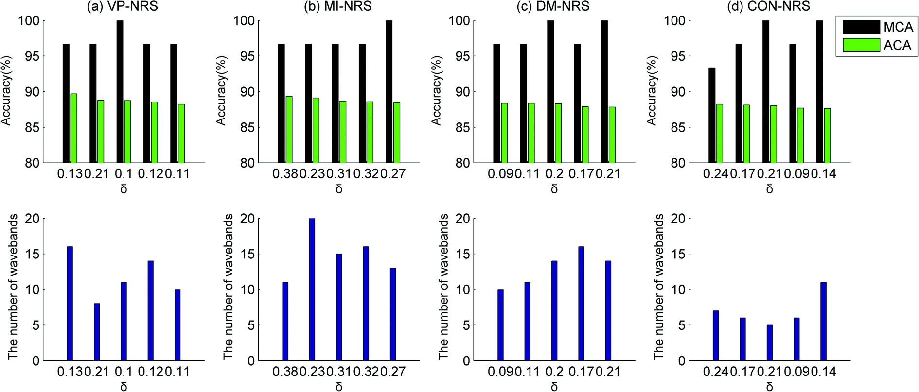
This dataset consisted of 120 healthy and 120 contaminated samples (30 samples each of Cu, Pb, Cd, and Zn contamination). For the 240 samples, 180 samples were assigned to training sets and 60 samples were assigned to testing sets. The dataset was employed to investigate the model's ability to identify healthy samples from samples contaminated with different heavy metals. The identification results were shown in Fig. 14.

Fig. 14 Identification results of healthy samples and different contamination samples.

The identification models achieved a satisfactory performance, as indicated by the MCA of over 95%. All ACA values were all above 90%, except for the DM-NRS algorithm when δ was 0.36. The results showed that the model can be used to distinguish contaminated samples from healthy samples. The CON-NRS algorithm selected a lower number of wavebands than the other waveband selection algorithms. The minimum number of wavebands selected by the CON-NRS algorithm was 7, with an ACA of 90.63% and an MCA of 95%. For an example, with a result of classification accuracy 91.67%, 4 healthy samples were identified as contaminated, and 1 contaminated sample was identified as healthy. For an identification model, if misclassification did exist, it was expected that the model could identify healthy samples as contaminated samples, for which it did not cause any food safety issues. The model explored in this study followed that characteristic.

4. Conclusions

Due to toxicity, accumulation, and difficulty in the degradation of heavy metals, improving the detection ability of shellfish contaminated by heavy metals has become a necessity to ensure consumer safety. In this study, the HSI technology was evaluated as a means to distinguish healthy samples of Ruditapes philippinarum from those contaminated with heavy metals. Compared with traditional laboratory-based techniques, HSI was a fast and convenient technique. The HSI system was portable and easy to use in the field. The findings of this study could provide technical support for the safety and quality management of shellfish products.

In this study, Ruditapes philippinarum were exposed to high concentrations of heavy metals for a short time. The concentrations of heavy metals in the cultured Ruditapes philippinarum were much higher than those found in polluted seawater. Therefore, the heavy metal content in the Ruditapes philippinarum may also be much higher than that in Ruditapes philippinarum harvested from polluted seawater. In future work, it should be studied further about the model's ability to distinguish Ruditapes philippinarum reared in progressively lowered concentrations of heavy metals.

Conflicts of interest

There are no conflicts of interest to declare.

Acknowledgements

This work was supported by the National Natural Science Foundation of China [grant number 62005109], Guangdong Basic and Applied Basic Research Foundation [grant numbers 2020A1515011368, 2021A1515012440], Technology Innovation Strategy Fund Project of Guangdong Province [grant number 2018A03017], Characteristic Innovation Projects of Universities in Guangdong Province [grant numbers 2019KTSCX094, 2019KQNCX074], Lingnan Normal University Nature Science Research Project [grant numbers ZL1902, ZL2007], Young Innovative Talents Training Program for Universities of Heilongjiang Province [grant number UNPYSCT-2018143].

References

1. G. Esposito, D. Meloni, M. C. Abete, G. Colombero, M. Mantia and P. Pastorino, et al., The bivalve Ruditapes decussatus: A biomonitor of trace elements pollution in Sardinian coastal lagoons (Italy), Environ. Pollut., 2018, 242, 1720–1728.
2. Z. Li, L. Pan, R. Guo, Y. Cao and J. Sun, A verification of correlation between chemical monitoring and multi-biomarker approach using clam Ruditapes philippinarum and scallop Chlamys farreri to assess the impact of pollution in Shandong coastal area of China, Mar. Pollut. Bull., 2020, 155, 111155.
3. M. H. Hu, X. J. Chen, P. C. Ye, X. Chen, Y. J. Shi and G. T. Zhai, et al., Combination of multiple model population analysis and mid-infrared technology for the estimation of copper content in Tegillarca granosa, Infrared Phys. Technol., 2016, 79, 198–204.
4. X. Chen, K. Liu, J. Cai, D. Zhu and H. Chen, Identification of heavy metal-contaminated Tegillarca granosa using infrared spectroscopy, Anal. Methods, 2015, 7(5), 2172–2181.
5. S. M. Elgammal, M. A. Khorshed and E. H. Ismail, Determination of heavy metal content in whey protein samples from markets in Giza, Egypt, using inductively coupled plasma optical emission spectrometry and graphite furnace atomic absorption spectrometry: A probabilistic risk assessment study, J. Food Compos. Anal., 2019, 84, 103300.
6. L. Yuan, X. Chen, Y. Lai, X. Chen, Y. Shi and D. Zhu, et al., A novel strategy of clustering informative variables for quantitative analysis of potential toxics element in Tegillarca granosa using laser-induced breakdown spectroscopy, Food Anal. Methods, 2018, 11(5), 1405–1416.
7. W. Wang, J. Yang, Q. Li, R. Ji, X. Gong and L. Li, Development of calibration models for rapid determination of chemical composition of Pacific Oyster (Crassostrea gigas) by near infrared reflectance spectroscopy, J. Shellfish Res., 2015, 34(2), 303–309.
8. X. Chen, L. Yuan, X. Chen, Y. Shi and D. Zhu, A strategy for rapid identification of healthy Tegillarca granosa from among those contaminated with unspecified heavy metals using infrared spectroscopy, Anal. Methods, 2017, 49(30), 4447–4454.
9. L. Li, S. Xie, J. Ning, Q. Chen and Z. Zhang, Evaluating green tea quality based on multisensor data fusion combining hyperspectral imaging and olfactory visualization systems, J. Sci. Food Agric., 2019, 99, 1787–1794.
10. L. Guo, Y. Yu, H. Yu, Y. Tang, J. Li, Y. Du, Y. Chu, S. Ma, Y. Ma and X. Zeng, Rapid quantitative analysis of adulterated rice with partial least squares regression using hyperspectral imaging system, J. Sci. Food Agric., 2019, 99, 5558–5564.
11. F. Tao, H. Yao, F. Zhu, Z. Hruska, Y. Liu and K. Rajasekaran, et al., A rapid and nondestructive method for simultaneous determination of aflatoxigenic fungus and aflatoxin contamination on corn kernels, J. Agric. Food Chem., 2019, 67(18), 5230–5239.
12. Y. Liu, H. Pu and D. W. Sun, Hyperspectral imaging technique for evaluating food quality and safety during various processes: A review of recent applications, Trends Food Sci. Technol., 2017, 69, 25–35.
13. J. Qin, F. Vasefi, R. S. Hellberg, A. Akhbardeh, R. B. Isaacs and A. G. Yilmaz, et al., Detection of fish fillet substitution and mislabeling using multimode hyperspectral imaging techniques, Food Control, 2020, 114, 107234.
14. J. H. Cheng and D. W. Sun, Hyperspectral imaging as an effective tool for quality analysis and control of fish and other seafoods: Current research and potential applications, Trends Food Sci. Technol., 2014, 37(2), 78–91.
15. M. Al-Sarayreh, M. M. Reis, W. Q. Yan and R. Klette, Potential of deep learning and snapshot hyperspectral imaging for classification of species in meat, Food Control, 2020, 117, 107332.
16. X. Zhu and G. Li, Rapid detection and visualization of slight bruise on apples using hyperspectral imaging, Int. J. Food Prop., 2019, 22(1), 1709–1719.
17. D. Wu, X. Chen, F. Cao, D. W. Sun, Y. He and Y. Jiang, Comparison of infrared spectroscopy and nuclear magnetic resonance techniques in tandem with multivariable selection for rapid determination of ω-3 polyunsaturated fatty acids in fish oil, Food Bioprocess Technol., 2014, 7(6), 1555–1569.
18. P. Baranowski, W. Mazurek and J. Pastuszka-Woźniak, Supervised classification of bruised apples with respect to the time after bruising on the basis of hyperspectral imaging data, Postharvest Biol. Technol., 2013, 86, 249–258.
19. D. Ye, L. Sun, W. Tan, W. Che and M. Yang, Detecting and classifying minor bruised potato based on hyperspectral imaging, Chemom. Intell. Lab. Syst., 2018, 177, 129–139.
20. C. Rogel-Castillo, R. Boulton, A. Opastpongkarn, G. Huang and A. E. Mitchell, Use of near-infrared spectroscopy and chemometrics for the nondestructive identification of concealed damage in raw almonds (Prunus dulcis), J. Agric. Food Chem., 2016, 64(29), 5958–5962.
21. M. M. Mafarja and S. Mirjalili, Hybrid binary ant lion optimizer with rough set and approximate entropy reducts for feature selection, Soft Comput., 2019, 23(15), 6249–6265.
22. Y. Liu, H. Xie, K. Tan, Y. Chen, Z. Xu and L. Wang, Hyperspectral band selection based on consistency-measure of neighborhood rough set theory, Meas. Sci. Technol., 2016, 27(5), 055501.
23. Q. Hu, D. Yu, J. Liu and C. Wu, Neighborhood rough set based heterogeneous feature subset selection, Inf. Sci., 2008, 178(18), 3577–3594.
24. Y. Liu, H. Xie, Y. Chen, K. Tan, L. Wang and W. Xie, Neighborhood mutual information and its application on hyperspectral band selection for classification, Chemom. Intell. Lab. Syst., 2016, 157, 140–151.
25. Y. Liu, H. Xie, L. Wang and K. Tan, Hyperspectral band selection based on a variable precision neighborhood rough set, Appl. Opt., 2016, 55, 462–472.
26. F. Macedo, M. Rosário Oliveira, A. Pacheco and R. Valadas, Theoretical foundations of forward feature selection methods based on mutual information, Neurocomputing, 2019, 325, 67–89.
27. D. B. Heras, F. Argüello and P. Quesada-Barriuso, Exploring ELM-based spatial–spectral classification of hyperspectral images, Int. J. Remote Sens., 2014, 35(2), 401–423.
28. C. Cheng, W. P. Tay, and G. B. Huang, Extreme learning machines for intrusion detection, in the 2012 International joint conference on neural networks (IJCNN), IEEE, 2012, pp. 1–8.

---