Effect of amorphous cellulose on the deformation behavior of cellulose composites: molecular dynamics simulation

Abstract

This study was aimed at predicting and enhancing the properties of the blend, as well as exploring the mechanism, of a polylactic acid (PLA)/amorphous cellulose composite system through molecular characterization. The static properties of the amorphous cellulose/PLA blend model and the mechanical response of the material under uniaxial tension were studied by molecular dynamics simulation to establish the structure–property relationship. PLA and cellulose showed poor miscibility, the change in the compatibility of the mixture can be attributed to the hydrogen bond interaction between the cellulose and PLA functional groups. The radius of gyration, interaction and free volume of the molecular chain in the blend were analyzed. The conformational changes under tensile deformation indicated that the load-bearing role of cellulose in the system was the main reason for increasing the strength of the material. The yield process was considered to be the infiltration of free volume caused by deformation.

---

1 Introduction

Natural fiber reinforced polymer composites are designed to creating low cost, high performance and lightweight materials to replace commonly used petroleum derived polymers.¹ Although polylactic acid (PLA) and cellulose belong to the class of biodegradable polymers, the drawbacks of PLA such as high cost, low crystallization rate, poor toughness and slow degradation rate limit its further application.² The synthesis of biodegradable and environmentally friendly composites could be achieved by improving the mechanical and thermal properties and crystallinity of PLA using the addition of cellulose.^3,4 For examples, Bagheriasl et al.⁵ found that the Young's modulus of PLA composites containing 6 wt% cellulose nanocrystal increased up to 23% compared with pure PLA. Purnama et al.⁶ prepared the bio-based composite of stereocomplex polylactide containing cellulose nanowhiskers with improved mechanical properties up to 2.70 GPa (Young's modulus) and thermal degradation temperature.

Cellulose is the most abundant renewable and biodegradable natural polymer in the biosphere and is one of the most commonly used polysaccharides in industry.⁷ The aggregate structure of cellulose is a complex system composed of an amorphous region and an interwoven crystalline region, wherein the crystalline region has no obvious boundary with the amorphous region but a gradual transitional region process. Molecules in the crystalline zone are orderly and stable arranged and bound together, so they have high mechanical strength.^8,9 In the amorphous region, the molecules are arranged irregularly, with more cracks and holes, showing lower strength and larger deformation.¹⁰ The mechanical properties of cellulose depend to some extent on the ratio between the crystalline and amorphous phases.

The properties of the material depend on the conformational characteristics of each chain and its interaction.^11,12 A large amount of research has focused on crystalline cellulose,^13,14 but contrary to the great efforts to characterize the crystal structure of cellulose, the amorphous region lacks structural exploration. Structural information on amorphous cellulose is limited.

Molecular simulation technology plays an increasingly important role in material design for studying the material properties and interactions of fillers and polymer matrices at the atomic scale,^15,16 to provide details of microscopic information or molecular interactions within the material, characterizing polymer compatibility.^17,18 It can reveal potential mechanisms that are not available or difficult to be obtained by experiments, guide the formulation of composite materials, and provide theoretical predictions and scientific evidence. It complements the deficiencies in the experiment to predict the nature of new materials that are already used or to be studied.

In this study, the changes in mechanical properties and miscibility caused by the addition of amorphous cellulose to the PLA matrix were investigated by using the atomic modeling technique. In order to explore the mechanism of action of amorphous cellulose on materials, the radius of gyration was calculated to analyze its conformation, and the radial distribution function was used to evaluate the structural properties of blends. The change of molecular interaction between cellulose and PLA was examined. The contribution of free volume to the blend was also investigated (Fig. 1).

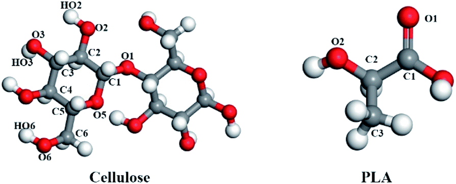Fig. 1 The structural unit of PLA and cellulose, the red is oxygen atoms, the gray is carbon atoms, the white is hydrogen atoms.

2 Experimental

2.1 Model and simulation method

All MD simulations were carried out using the Materials Studio 7.0 package with the COMPASS II force field.¹⁹ Five systems with different weight fractions of cellulose (0%, 10%, 20%, 30% and 100%) were considered. One of the important choices in polymer modeling is the number of repeating units of the polymer chain in the cubic unit modeled. The specific length of the chain is mainly determined by two factors. Firstly, the length of the chain was chosen to be sufficient to eliminate the sensitivity of the molecular weight of the polymer chain to polymer properties. Secondly, the chain length of the polymer chain should be short enough to speed up the equilibrium process.²⁰ Previous studies determined the representative length by calculating the solubility parameters of PLA chains of different sizes and selecting a length above which the solubility parameter reached a constant value. When the number of repeating units of PLA exceeds 10, the solubility parameter tends to be stable.²¹ The model of amorphous region composed of cellulose chains of different lengths is not obvious in terms of molecular conformation or physical and chemical properties.^22,23 In this study, the degrees of polymerization of PLA and cellulose was set to 50 and 10. The parameters of the simulated blends are listed in Table 1.

Table 1 Details of the simulated blends

System no.	Degree of polymerization		No. of chains		Weight fraction, %		Density (g cm^−3)	Length of the box side, nm
	PLA	Cellulose	PLA	Cellulose	PLA	Cellulose
1	50	10	20	0	100.00	0.00	1.176	4.66
2	50	10	20	5	89.80	10.20	1.189	5.12
3	50	10	18	10	79.90	20.10	1.223	5.14
4	50	10	16	15	70.20	29.80	1.237	5.16
5	50	10	0	20	0.00	100.00	1.486	4.18

---

Initially, the bulk phases were constructed with the Amorphous Cell program, which combined the use of an algorithm developed by Theodorou and Suter²⁴ and the scanning method of Meirovitch.²⁵ The molecular chains were randomly loaded into a simulation box with a larger inter-chain spacing. This method was used for the construction of amorphous cellulose model.^22,23,26,27 Periodic boundary conditions (PBC) are used in all model constructions, which can simulate real systems through molecular models with smaller amount of atoms. A periodic cube box was filled with a chosen amount of PLA and cellulose chains of sufficiently low density.²⁶ After the initial construction, a 5000-step geometry optimization was performed on the constructed model to eliminate the local non-equilibrium structure with a convergence threshold of 0.001 kcal mol⁻¹ Å⁻¹. The models were carried out in the NPT ensemble for 2 ns at a pressure of 1 bar and a temperature of 500 K to ensure that the polymer was in a molten (amorphous) state (above the glass transition temperature of the material). In order to further relax local hot-spots and to allow the system to achieve equilibrium, the structures were subjected to the 5 cycles thermal annealing from 300 to 800 K and then back to 300 K with 50 K intervals. At each temperature, 100 ps of NPT MD simulation was performed at 1 bar. Then, the lowest energy configuration was selected for the molecular dynamics' calculation. Subsequently, the production MD simulations were carried out in the NVT ensemble for 5 ns at the temperature of 298 K, during which trajectories were stored, periodically, for the later post processing. The Nosé–Hoover^28,29 thermostat and Berendsen³⁰ thermostat were applied to keep the temperature and pressure constant. The long-range electrostatic interaction was calculated by the Ewald method with the accuracy of 0.001 kcal mol⁻¹ and the buffer width of 0.5 Å. The van der Waals interaction used the atom-based method, the cut-off distance was set to be 12.5 Å, the spline width was set to be 1 Å, the buffer width was set to be 0.5 Å and the time step was set to be 1 fs.

Choosing an appropriate force field is an important step in atomic simulation, which determines the accuracy of the material's atomic interaction and other properties. The COMPASS force field is a molecular force field suitable for condensed state applications. It can accurately predict the molecular structure, conformation, vibration and thermodynamic properties of condensed state molecules. The COMPASS potential function is expressed as:³¹

U = E_b + E_θ + E_ϕ + E_χ + E_b,b′ + E_b,θ + E_b,ϕ + E_θ,θ′ + E_θ,ϕ + E_θ,θ′,ϕ + E_i,j + E_Coul (1)

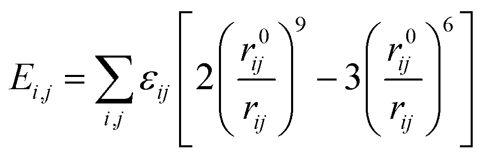
The functions can be divided into two categories of valence terms including diagonal and off-diagonal cross-coupling terms and nonbond interaction terms. The valence terms represented internal coordinates of bond (b), angle (θ), torsion angle (ϕ), and out-of-plane angle (χ), and the cross-coupling terms included combinations of two or three internal coordinates (E_b,b′, E_b,θ, E_b,ϕ, E_θ,θ′, E_θ,ϕ, E_θ,θ′,ϕ). Nonbond interactions included interactions between 9 to 6 Lennard-Jones potentials of the van der Waals term and coulomb functions of the electrostatic term, being used for interactions between atomic pairs separated by two or more intermediate atoms or pairs belonging to different molecules. It has been applied to the simulation of PLA, cellulose, organic and inorganic molecules. In the previous research, the COMPASS force field had advantages in the expression of the mechanical properties of cellulose crystal.³² Table 2 lists the atomic charges for cellulose and PLA in COMPASS force field.

Table 2 The partial atomic charges of PLA and cellulose, in elementary charge unit (e)

	C1	O1	C2	O2	HO2	C3	O3	HO3	C4	C5	O5	C6	O6	HO6
Cellulose	0.107	−0.320	0.107	−0.570	0.410	0.107	−0.570	0.410	0.247	0.107	−0.320	0.054	−0.570	0.410
PLA	0.562	−0.450	0.107	−0.272	—	−0.159	—	—	—	—	—	—	—	—

---

2.2 Calculation of system properties

The free volume theory proposed by Fox and Hory is to refer to the holes between the molecules inside the material as free volume,³³ which mainly includes defects in the size of the polymer atoms and voids due to random packing of atoms. The value of the free volume fraction (FFV) was calculated using the following formula:where V_O = 1.3V_w is the occupied volume, V is the cell volume, and V_w is the van der Waals volume obtained from the van der Waals surface.³⁴ It should be noted that the FFV value obtained with a probe of radius 0 Å takes into account the smallest space that is not filled by polymer atoms.

The solubility parameter δ is defined as the square root of the cohesive energy density (CED) that describes the strength of the intermolecular forces of the system.^35,36

2.3 Equilibration

The equilibrium of all systems was monitored by potential energy and radius of gyration (R_g). The autocorrelation function of the radius of gyration of the system was shown in Fig. 2. The relaxation time corresponds to the time when the autocorrelation function of the radius of gyration is 1/e. The energy and radius of gyration of all systems were stable within the first 700 ps. According to the relaxation time, the simulation time was long enough for sampling to give enough independent configuration to fully average the static characteristics.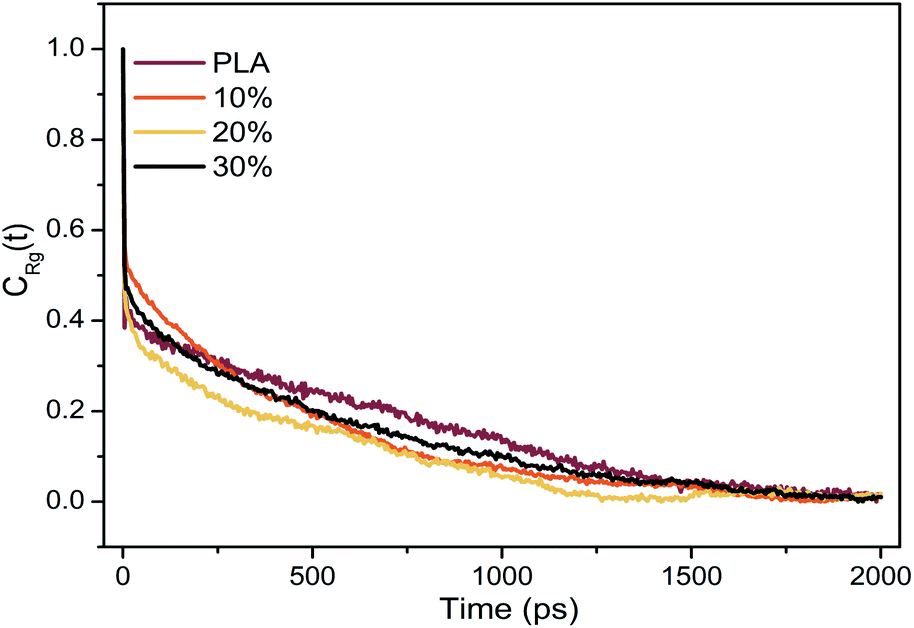

Fig. 2 Autocorrelation function of the radius of gyration.

3 Results and discussion

3.1 Static structure of composite materials

In the molecular chain of the polymer, the intermolecular force is actually a comprehensive reflection of various forces. Polymer molecular weight is very large, and has multiple dispersity, so the interaction between macromolecular chains cannot be expressed by a certain force. Generally, cohesive energy or cohesive energy density are commonly used to measure the force between macromolecules. The cohesive energy density (CED) refers to the total energy of a mole of molecules gathered together, or the energy required to overcome the intermolecular force that moves a mole of aggregated molecules out of its molecular gravity range.^35,36 Fig. 3 shows the cohesive energy density of the material. The energy contribution of the interaction of electrostatic (Elec) and van der Waals (vdW) to the cohesive energy density were studied.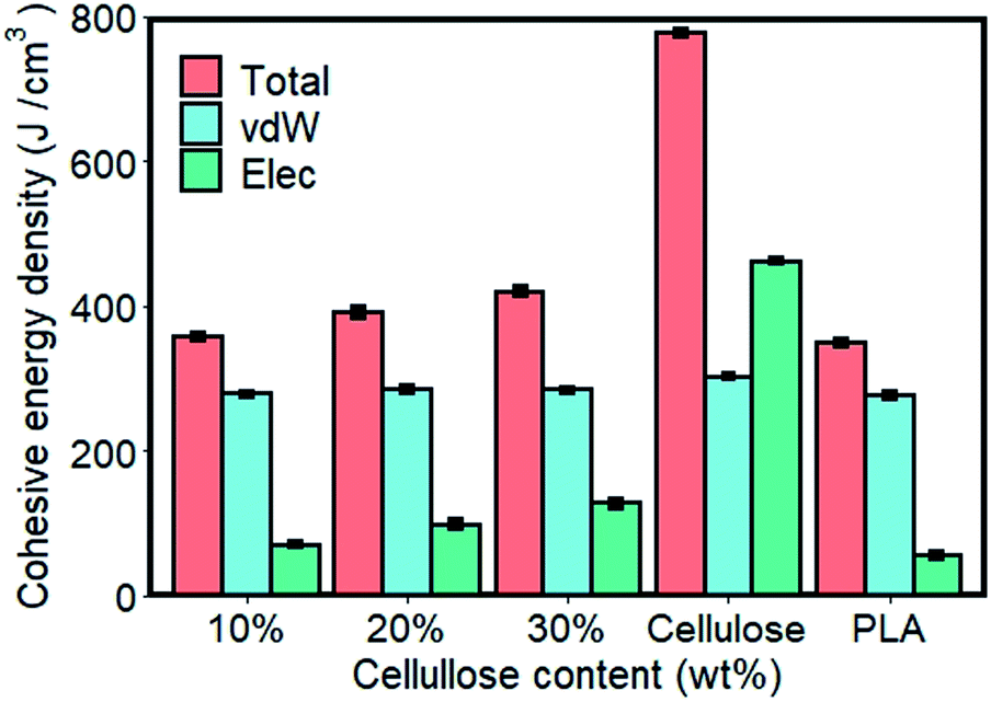

Fig. 3 Cohesive energy density and energy contribution of the materials.

As shown in Fig. 3, CED of cellulose calculated by MD simulation data was significantly higher than that of pure PLA. For composite materials, the value of CED laid between pure components and increased with the content of cellulose added. In order to further understand the cause of the difference in CED of materials, the energy contribution of CED decomposed into electrostatic and van der Waals components. Pure components and composite materials had nearly equal van der Waals strengths on CED, and the difference between them depended more on electrostatic interactions. Among them, the electrostatic interaction of cellulose was 46.97% stronger than that of vdW, and 727.99% higher than that of pure PLA. This was mainly due to the structure, in which hydrogen bonds can be formed within and between the molecules of cellulose. The increase in the cellulose content in the composite made the system to provide more sites for hydrogen bonding, resulting in increased intermolecular forces in the system. Hydrogen bond analysis further confirmed this observation.

Hydrogen bonding was detected from geometric standards; if the donor–acceptor distance was less than 3.5 Å and the hydrogen-donor–acceptor bond angle, i.e. H–O⋯O bond angle is less than 30°, they were considered to be hydrogen bonds.^37,38 The number of intramolecular and intermolecular hydrogen bonds between cellulose in a unit volume in the system is shown in Fig. 4a. The hydrogen bonds between cellulose and cellulose in composite materials mainly existed in the form of intramolecular hydrogen bonds. With 10 wt% cellulose, the intermolecular hydrogen bonds formed between cellulose and PLA, account for only 21.03% of the total, which was far lower than the intramolecular and intermolecular hydrogen bonds of cellulose. As the cellulose content increased, the contact between the cellulose molecular chains increased, and the ratio of intermolecular and intramolecular hydrogen bonds formed per unit volume increased significantly. However, the number of intermolecular hydrogen bonds formed by cellulose and PLA only increased slightly.

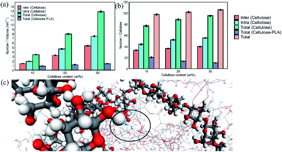Fig. 4 (a) The number of hydrogen bonds per unit volume in system. (b) The number of hydrogen bonds formed by each cellulose and surrounding molecule in the system. (c) The partial molecular snapshot of the composite material under 10 wt% cellulose. The ball-and-stick model is cellulose, the line model is PLA, the red is oxygen atoms, the gray is carbon atoms, the white is hydrogen atoms, and the blue dashed line is hydrogen bonds.

Interestingly, the number of intramolecular and intermolecular hydrogen bonds formed by each cellulose in the material is shown in Fig. 4b. The tendency of the number of hydrogen bonds formed by PLA and cellulose per unit volume in the system with the cellulose content was opposite to that formed by each cellulose and PLA. Although the number of hydrogen bonds in the material increased, the binding capacity between PLA and cellulose decreased. The number of hydrogen bonds formed by a single cellulose seems to be fixed, and PLA was not as competitive as cellulose to occupy the site of hydrogen bonds.

One of the reasons for the change in CED of the material was the hydrogen bonding interaction between the functional groups of the two polymers. Analysis of the radial distribution function (RDF) obtained from molecular models can provide insights into the contribution of interactions between different types of atomic pairs. It can provide the probability of finding other atoms at a distance r near the atom.³⁹

The RDF between the oxygen atom from PLA and the cellulose is shown in Fig. 5. As shown in Fig. 5a, the hydroxyl groups of O2H, O3H and O6H at the C2, C3 and C6 positions of cellulose showed a large peak at about 1.85 Å between the Od in PLA, indicating that –OH···O=C interaction, the peak distance indicated the most likely distance between hydrogen-bonded atoms. The hydroxyl group at the C6 position of cellulose had high activity due to small steric hindrance and showed the highest peak on the curve. In addition, as the amount of cellulose increased, the peak area decreased significantly, indicating that the spatial correlation between them decreased. The value of the RDF corresponding to Od–CH in the distance before the sum of the vdW radii of H and O was zero, showing a small peak at 2.90 Å, indicating that the interaction between them is more in the form of vdW force.

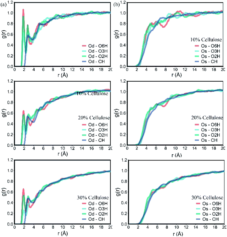Fig. 5 RDF between the oxygen atom O from PLA and the cellulose: (a): double bond oxygen atom Od; (b): single bond oxygen atom Os.

The spatial correlation between the single-bonded oxygen atom Os in PLA (Fig. 5b) and the groups in cellulose was obviously weaker than the double-bonded oxygen atom, and there were small peaks or few peaks between them. With the increase of cellulose content, this spatial correlation gradually disappeared. At 30% cellulose content, there was almost no obvious peak in the curve. The interaction between PLA and cellulose was mainly composed of the electrostatic force between the double bond oxygen atom Od and cellulose OH in PLA, and the van der Waals force between molecular chains. With the increase of cellulose, this interaction weakened and the bonding between atoms impaired.

It was also verified the CED using the free volume fraction (FFV). Fig. 6 shows the free volume distribution of the materials. It should be noted that the FFV value obtained with a probe of radius 0 Å took into account the smallest space that was not filled by polymer atoms. It can be seen that pure PLA had the highest FFV of 21.30%, and there was a large amount of free volume in the system. The FFV value decreased with the increase of cellulose content, indicating that the addition of cellulose can make the material denser. Combined with the results of CED and hydrogen bonds, the value of CED reflected the intermolecular energy between cellulose–cellulose, PLA–PLA, and PLA–cellulose molecules. With the increase of cellulose content, the intermolecular interaction of the material increased, and the cellulose can form intermolecular hydrogen bonds with PLA and itself, so that the material formed an entangled network structure, and the distance between molecules was shortened, thus making the system more dense.

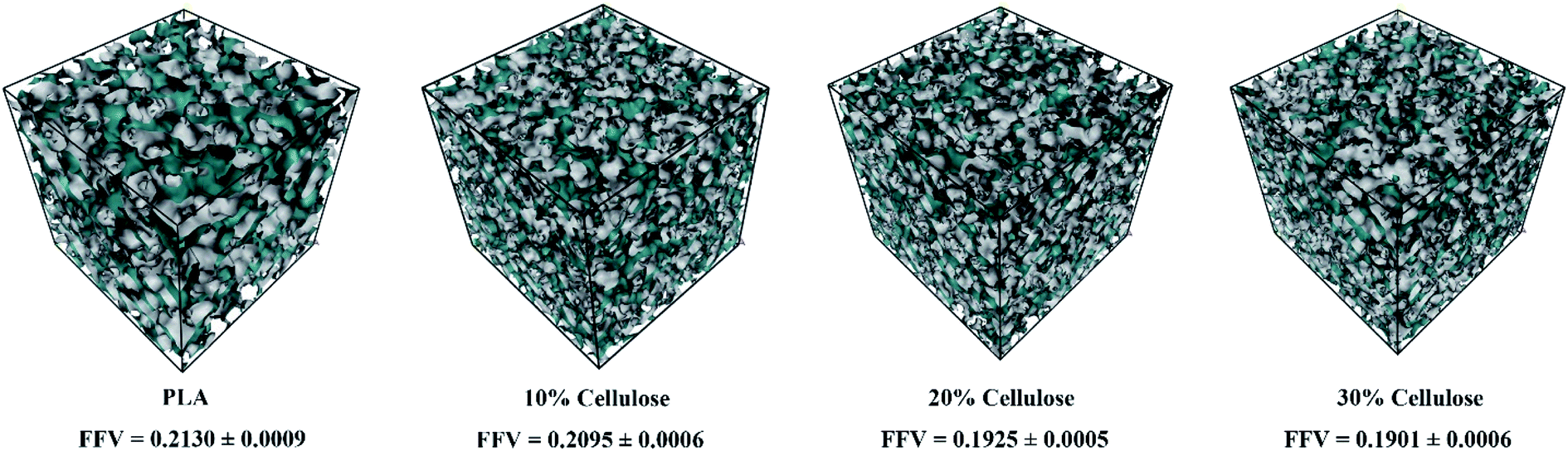Fig. 6 The free volume distribution of the materials. The green area represents the free volume and the grey area represents the volume of polymer materials.

3.2 Compatibility of composite materials

The δ of pure PLA calculated by MD was 18.66 ± 0.07 (J cm⁻³)^0.5, which was underestimated by 1.79% compared to the lower value in the experimental range (19–20.50 (J cm⁻³)^0.5).^40–43 This behavior was also observed in several polymers such as PHB, PPDO, PAM and PVPh.^35,44,45 The δ of amorphous cellulose was 27.86 ± 0.05 (J cm⁻³)^0.5, which was 4.91% lower than the δ of microcrystalline cellulose 29.30 (J cm⁻³)^0.5.⁴⁶ This is predictable because the crystallization zone cellulose structure is more stable than the amorphous zone. The more mismatches in the solubility parameters between the pure components, the more unfavorable the energy changes during mixing.⁴⁷ For weakly interacting polymers, this difference should not exceed 2 (J cm⁻³)^0.5.⁴⁸ Clearly, PLA is immiscible with cellulose.

For binary polymer systems, the intermolecular distribution function has been used to determine the degree of miscibility of polymer blends. Miscibility occurred when the heterogeneous contact between the two components in the mixture reached a higher g(r) value than the contact between the same components.⁴⁴ If PLA and cellulose were completely miscible, the PLA–cellulose curve was above the PLA–PLA and cellulose–cellulose curve. In the case of immiscibility, the PLA–cellulose curve would lie below the two curves. Fig. 7 shows the RDF between all types of PLA and cellulose atoms in the system. Here an intermediate situation was observed, which meant that PLA and cellulose were semi-miscible in the length range of 2 nm. Because of the stronger interaction between celluloses, the cellulose–cellulose curve was higher than the other two curves. As the cellulose content increased, the difference between the PLA–PLA, PLA–cellulose and cellulose–cellulose curves further expanded, and the PLA–cellulose curve was at the bottom. Therefore, within this length range, PLA and cellulose were immiscible, which also meant that the miscibility of PLA and cellulose depended on the scale. Fig. 7 shows a typical snapshot of a blend of PLA and cellulose, which clearly showed the distribution of cellulose and PLA molecular chains in the blend. Combining the results in the CED, as the cellulose content increased, the probability of contact between cellulose chains increased dramatically. Compared with PLA, cellulose may form a more stable connection through hydrogen bond interaction with each other, and cellulose cannot provide sufficient hydrogen bonding sites for PLA. The change in compatibility of the mixture can be attributed to the hydrogen bonding interaction between the functional groups of the two polymers.

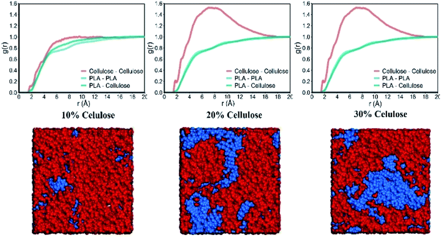Fig. 7 The RDF of PLA–PLA, PLA–cellulose and cellulose–cellulose in the system, and snapshots of PLA and cellulose blends. Cellulose and PLA chains are colored in blue and red.

3.3 Mechanical behavior of composite materials

The stress–strain curve of the tensile deformation of pure PLA and composite materials is depicted in Fig. 8. In this work, the strain rate was set to be 10⁸ s⁻¹. At this strain rate, PLA exhibited obvious plastic behavior and strain hardening. In practice, PLA is usually hard and brittle, showing brittle fracture. This difference may be that the molecular weight of the simulated polymer cannot reach the molecular weight of the actual polymer. The structure used in theoretical estimation is often ideal, and sufficient entanglement cannot be achieved. In practice, it was found that PLA changed from brittleness to toughness after the pre-stretching or quenching treatment.⁴⁹ Therefore, these estimated elastic limits cannot be directly compared with experimental values. Nevertheless, the relative elastic limits in the simulations and experiments should be comparable. In this study, only the elastic stage and yield behavior of the composite material were discussed.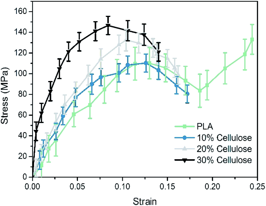

Fig. 8 The stress–strain curves of materials.

The results showed that the Young's modulus of the PLA matrix was 1.14 ± 0.16 GPa, the yield stress was 109.68 ± 15.92 MPa. The Young's modulus of the composites was 1.71 ± 0.24 GPa, 1.81 ± 0.11 GPa and 2.02 ± 0.20 GPa, respectively, which had a great improvement as the cellulose content increased. The Young's modulus of the system at the 30% cellulose content was 80.70% higher than that of the PLA matrix. In terms of yield stress, it was increased by 31.12% compared to the PLA matrix.

The evolution of the microstructure can be used to explain the difference in the stress–strain response.⁵⁰ Fig. 9 shows the structural evolution of the material during stretching, in which, only the representative molecular chains in the model are presented. For the PLA matrix, the polymer chain stretched in the stretching direction, and the end-to-end distance increased from 34.89 Å to 40.40 Å. In the composite material, the variation trend of the end-to-end distance between the cellulose molecular chains and the PLA molecular chains under different cellulose content was different. The different configurations of polymer chains were the possible reasons for their different stress–strain responses. For this reason, the changes in the radius of gyration (R_g) and the mean square end-to-end distance (H_end-to-end) of the cellulose and PLA molecular chains with respect to 0 strain case are shown in Fig. 10.

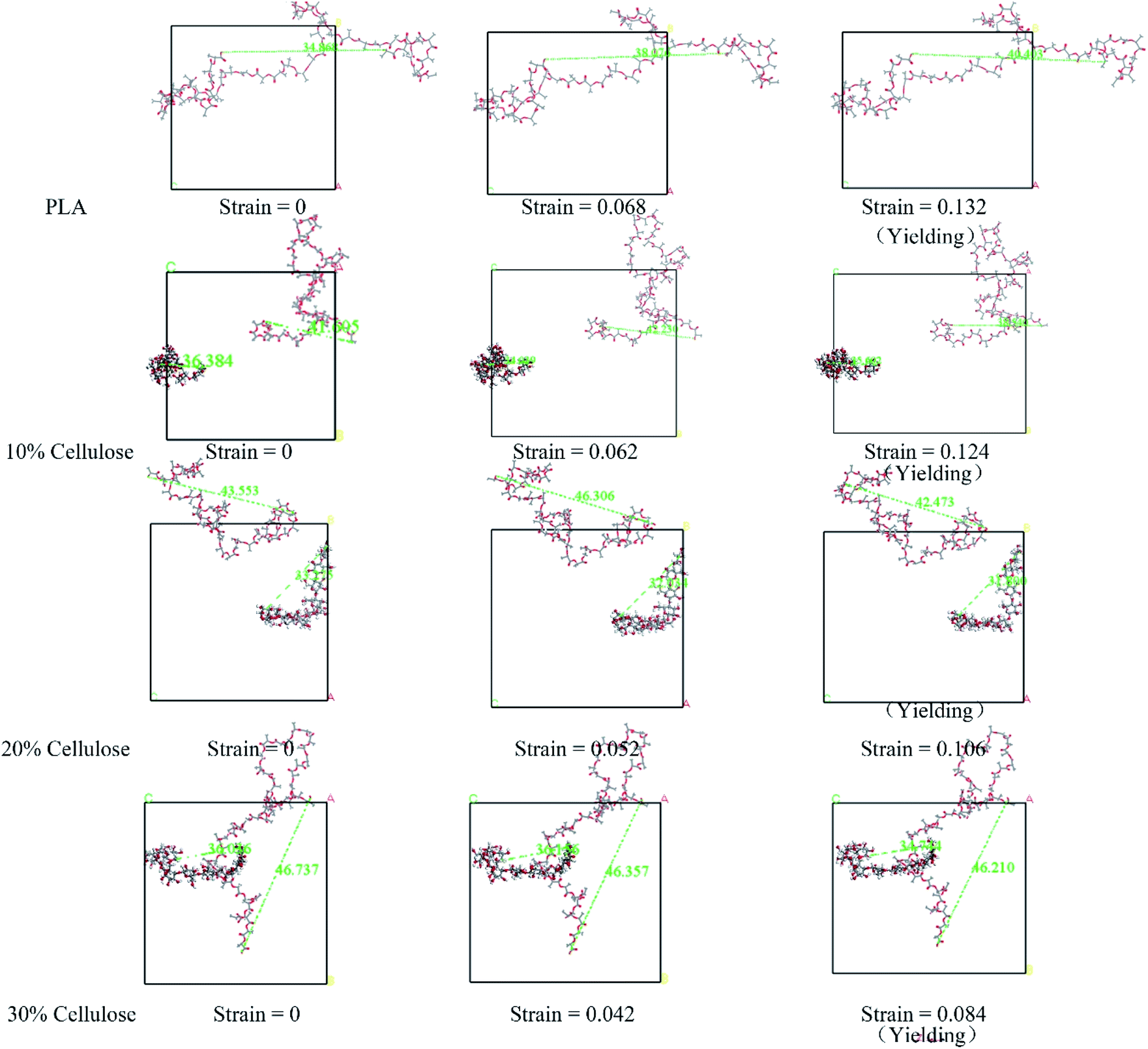Fig. 9 The structural evolution of the material during stretching. The ball-and-stick model is cellulose, the line model is PLA, and the green dotted line is the end-to-end distance of the molecular chain.

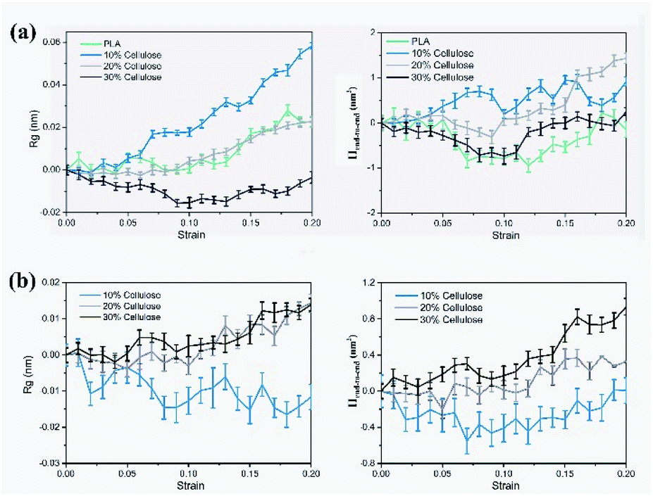Fig. 10 Evolution of the radius of gyration (R_g) and mean square end-to-end distance (H_end-to-end), relative to the 0 strain case: (a) PLA; (b) cellulose.

The results showed that in the PLA matrix, the configuration of the PLA molecular chain did not change significantly at the initial stage of tensile deformation, and the R_g of the molecular chain increased significantly near the yield point. After adding cellulose, as the cellulose content increased, the R_g and H_end-to-end of the cellulose molecular chain increased significantly, while the PLA molecular chain decreased to a certain extent. Cellulose itself had high strength. Adding cellulose to the PLA matrix can effectively bear part of the stress, reduce the stretching of the PLA molecular chain, and improve the strength of the material.

Generally, the yield behavior of a material is related to the generation of voids in the system with tensile deformation.⁵¹ In order to investigate the yield mechanism of the system from the molecular scale, the change of free volume in the system was studied. The snapshot of the free volume distribution near the cellulose molecular chain in the 10 wt% cellulose is shown in Fig. 11.

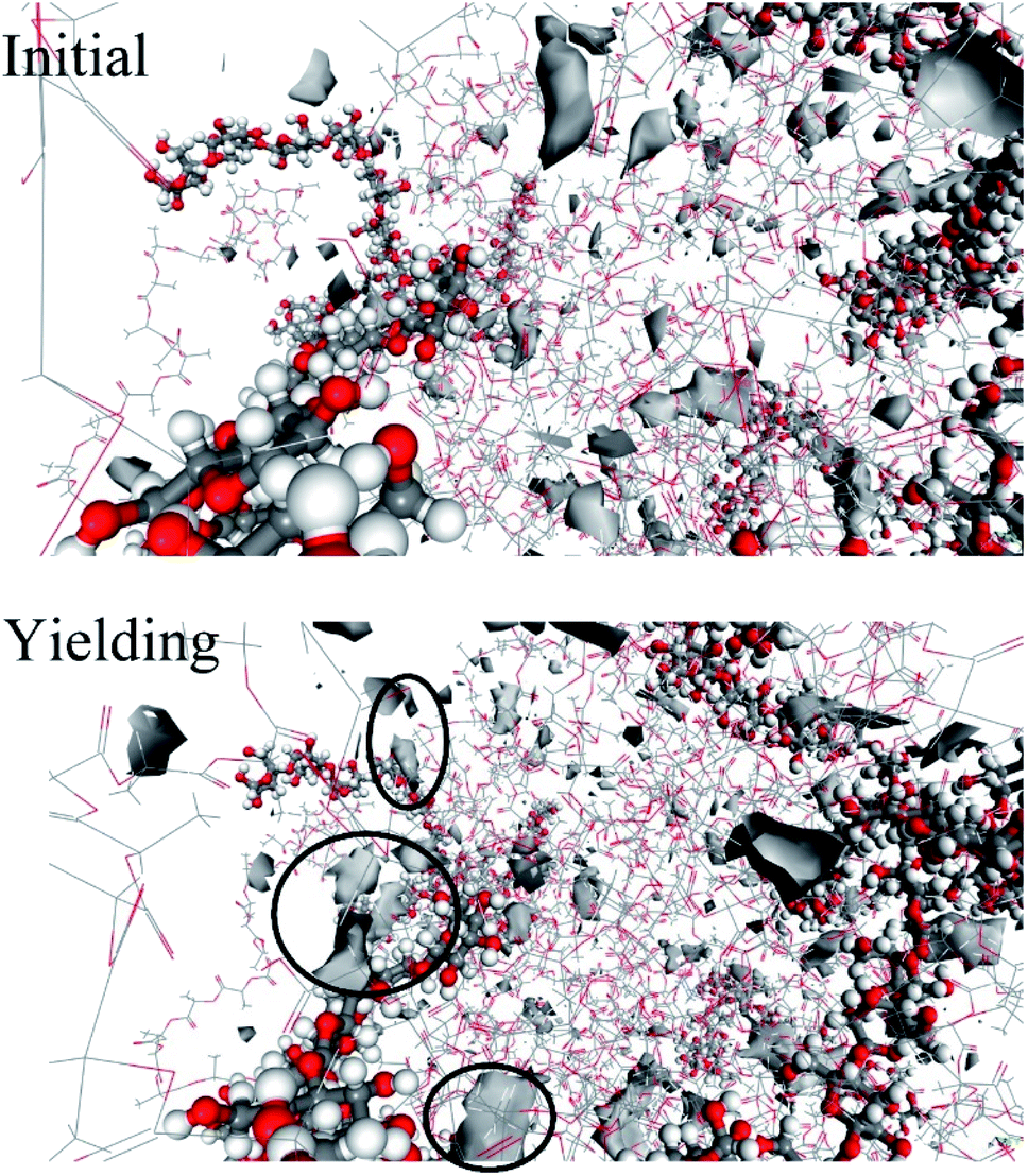Fig. 11 The snapshot of the free volume distribution near the cellulose molecular chain before and after yielding in 20 wt% cellulose.

There was a certain amount of free volume near the cellulose molecular chain, and the amount of free volume increased with the stretching process. Usually, the size of the free volume depends on the size of the test particles scanning the free volume area. The applied methods to obtain free volume data from the experimentally observed PALS spectra due to respective corrections were supposed to be related with the real size of holes starting from a cutoff radius of about 1.1 Å, which was the size of a positronium molecule.⁵² In this study, the total free volume in the material was calculated using a grid with a grid step of δ = 0.7 and a probe molecular radius of 1.1 Å (the size of the positronium molecule). The change in free volume with strain is shown in Fig. 12. Before yielding, the free volume of the system maintained a relatively low growth rate. Near the yield point, the free volume of the system increased sharply. There may be a threshold for the generation of free volume in the system. Before reaching the threshold, the free volume of the system rose almost in accordance with the Hooke elastic behavior. When the threshold was reached, the system instantaneously generated a large number of holes and then yielded.

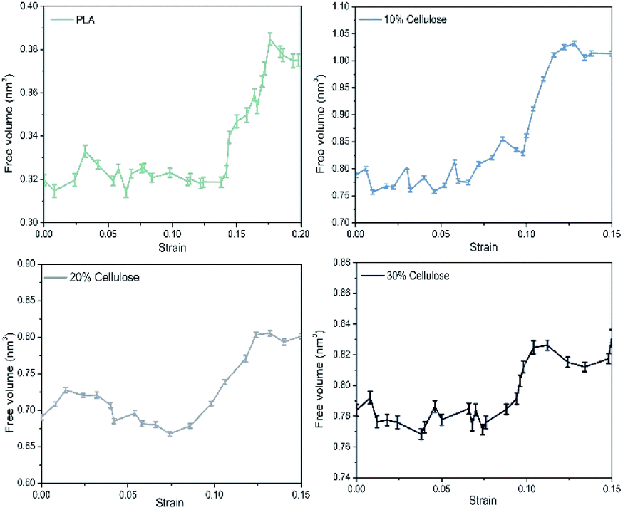Fig. 12 Evolution of free volume in the materials with strain.

To further reveal the enhancement mechanism of cellulose in the material, Fig. 13a and b depict the corresponding changes in potential energy and valence interactions. The potential energy of a system can be expressed as a sum of valence (or bond), crossterm, and non-bond interactions. The energy of valence interactions is generally accounted for by diagonal terms: bond stretching (bond), valence angle bending (angle), dihedral angle torsion (torsion), inversion, also called out-of-plane interactions terms, which are part of nearly all force fields for covalent systems. The curve change can be explained by inter-chain and intra-chain phenomena. For pure PLA, the change of potential energy during tensile deformation was mainly related to the increase of non-bond energy. This confirmed the common belief that stretching an amorphous polymer would cause its chain arrangement to increase continuously, which in turn led to the formation of more inter-chain van der Waals contacts and continuous monotonic changes in non-bonding energy.⁵³ After adding cellulose to the PLA matrix, the contribution of non-bonding energy to the change of potential energy gradually decreased during the gradual deformation of the material, and the change of potential energy was mainly related to the increase of valence interaction. Specifically, the energy changes of bonds, angle and inversion angle were negligible. In contrast, the dihedral energy experienced a considerable strain rate-dependent change, possibly due to the gradual rotation of C–C bonds to transmute gauche conformations to the lower-energy trans conformations. Combining the free volume in the material and CED, due to the relatively low packing density and intermolecular interactions in pure PLA, molecular chains obtained greater mobility and contact between molecules was easier. After the cellulose was incorporated, the molecular chain was fixed to a certain extent, which depended more on the changes within the chain.

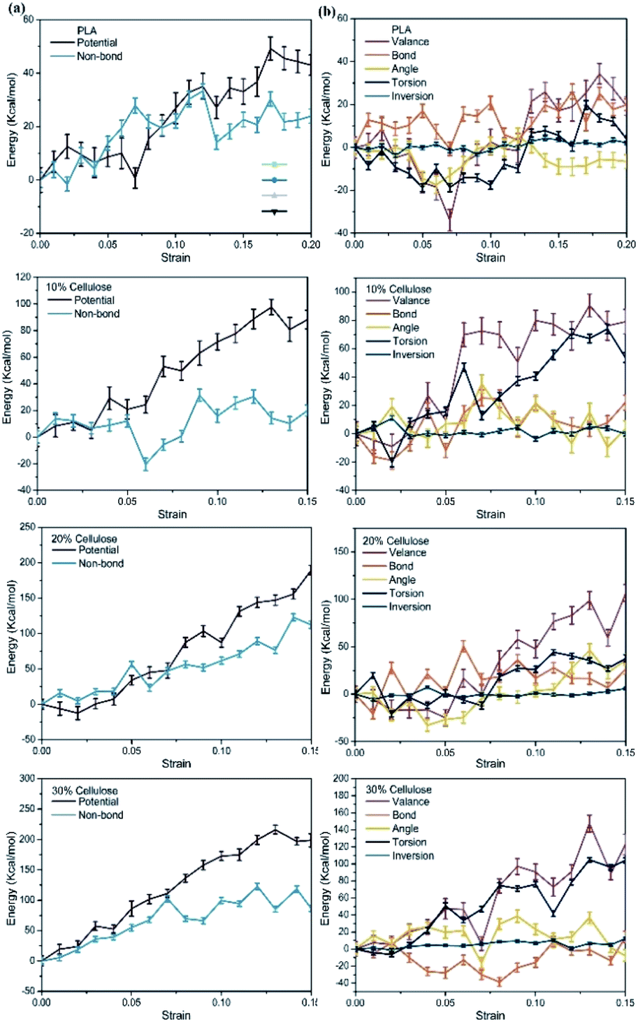Fig. 13 Evolution of energy with strain in the materials, relative to the 0 strain case: (a) potential energy; (b) valence energy.

In addition, the effects of three strain rates of 10⁸ s⁻¹, 10⁹ s⁻¹, and 10¹⁰ s⁻¹ on the mechanical properties of materials were also considered. Fig. 14 shows the stress–strain curve of the material at three strain rates with 20% cellulose content. The stress–strain curve had a similar changing trend. As the strain rate increased, the Young's modulus and yield stress of the material increased. When the maximum strain rate was 10¹⁰ s⁻¹, the yield stress reached 188.92 ± 11.79 MPa, the Young's modulus was 2.66 ± 0.15 GPa and the lower strain rate (10⁸ s⁻¹) yield stress was 132.52 ± 10.44 MPa and Young's modulus was 1.81 ± 0.11 GPa. At different strain rates, the free volume curves of the materials were similar and did not show a significant difference (Fig. 14b). In addition, the energy of models with different strain rates was calculated (Fig. 14c–f). It can be seen that the change of energy mainly depended on the change of non-bonding energy. The bond energy and the angle energy remained relatively constant throughout the entire range of deformation, and the torsion angle energy change exhibited a considerable strain rate dependence. A lower strain rate allowed the polymer chain to obtain a greater mobility, and at a higher deformation rate, because the degree of relaxation of atoms was smaller and the polymer chains would hinder each other's movement, thereby increasing the yield stress.

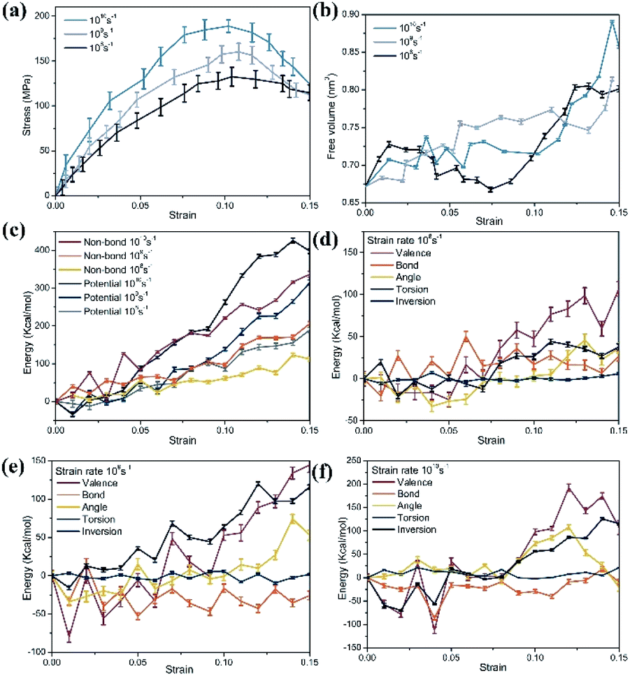Fig. 14 (a) Stress–strain curve of 20% cellulose content composite material at three strain rates; (b) free volume evolution; (c) potential and non-bonding energy evolution at three strain rates, relative to the 0 strain case; (d) energy evolution at the strain rate of 10⁸ s⁻¹, relative to the 0 strain case; (e) energy evolution at the strain rate of 10⁹ s⁻¹, relative to the 0 strain case; (f) energy evolution at the strain rate of 10¹⁰ s⁻¹, relative to the 0 strain case.

4 Conclusions

In this work, PLA composites were reinforced by adding amorphous cellulose to enhance their mechanical properties. Using MD simulation, the molecular details of PLA combined with amorphous cellulose and the mechanical properties of composite materials under the tensile deformation were studied.

After the amorphous cellulose was added to the PLA matrix, the composite material had a stronger intermolecular force due to the formation of intermolecular and intramolecular hydrogen bonds of cellulose, resulting in a denser structure. As the cellulose content increased, the repulsion between PLA and cellulose increased due to the poor compatibility between cellulose and PLA.

In the process of tensile deformation of PLA, non-bonding interaction played an important role. As the deformation progressed, the arrangement of its chains increased, which in turn led to more van der Waals contacts between chains. The movement of the molecular chain was accompanied by the rapid micro-cavitation, which in turn provided space for the change of the molecular chain. The yield of the material was the result of the evolution of free volume.

After the addition of cellulose, the material had a more improvement in young's modulus than PLA. In the process of stretching, the PLA molecular chain configuration in the composite material did not change significantly, but the cellulose chain configuration changed greatly, which was attributed to the strength of the cellulose itself and played a more bearing role in the system. There was not enough room for the movement of the molecular chain due to the more compact accumulation of composites. The energy change of the material was mainly based on valence interaction. Changes in the chain configuration such as bond angle bending and chain rotation were mainly related to significant changes in the energy associated with the torsion angle. These analyses helped to understand the interaction between cellulose/PLA composites and provided a theoretical basis for formulation design.

Conflicts of interest

There are no conflicts to declare.

Acknowledgements

The authors are grateful for financial support by the National Key R&D Program of China (2018YFD0600302). We are grateful for the support of related hardware and software computing resources provided by the National Supercomputing Center in Shenzhen.

Notes and references

1. K. Kummerer, Green Chem., 2007, 9, 899–907.
2. R. Auras, B. Harte and S. Selke, Macromol. Biosci., 2004, 4, 835–864.
3. D. Battegazzore, S. Bocchini, J. Alongi, A. Frache and F. Marino, Cellulose, 2014, 21, 1813–1821.
4. F. A. dos Santos, G. C. V. Iulianelli and M. I. B. Tavares, Polym. Eng. Sci., 2017, 57, 464–472.
5. D. Bagheriasl, P. J. Carreau, B. Riedl and C. Dubois, Polym. Compos., 2018, 39, 2685–2694.
6. P. Purnama and S. H. Kim, Polym. Degrad. Stab., 2014, 109, 430–435.
7. D. Klemm, B. Heublein, H.-P. Fink and A. Bohn, Angew. Chem., Int. Ed, 2005, 44, 3358–3393.
8. P. Zugenmaier, Prog. Polym. Sci., 2001, 26, 1341–1417.
9. Z. Benková and M. N. D. S. Cordeiro, Langmuir, 2015, 31, 10254–10264.
10. H. Montès, K. Mazeau and J. Y. Cavaillé, Macromolecules, 1997, 30, 6977–6984.
11. K. Mazeau, Carbohydr. Polym., 2011, 84, 524–532.
12. Y. Nishiyama, U. J. Kim, D. Y. Kim, K. S. Katsumata, R. P. May and P. Langan, Biomacromolecules, 2003, 4, 1013–1017.
13. G. Carrard, A. Koivula, H. Söderlund and P. Béguin, Proc. Natl. Acad. Sci., 2000, 97, 10342–10347.
14. S. P. Chundawat, G. Bellesia, N. Uppugundla, L. da Costa Sousa, D. Gao, A. M. Cheh, U. P. Agarwal, C. M. Bianchetti, G. N. Phillips Jr, P. Langan, V. Balan, S. Gnanakaran and B. E. Dale, J. Am. Chem. Soc., 2011, 133, 11163–11174.
15. J. Lu, D. M. Liu, X. N. Yang, Y. Zhao, H. X. Liu, H. Tang and F. Y. Cui, Appl. Surf. Sci., 2015, 357, 1114–1121.
16. N. Silvestre, B. Faria and J. N. C. Lopes, Compos. Struct., 2012, 94, 1352–1358.
17. A. Ahmadi and J. J. Freire, Polymer, 2009, 50, 4973–4978.
18. T. Ge, G. S. Grest and M. O. J. A. M. L. Robbins, 2013, 2, 882–886.
19. Accelrys, Accelrys Materials Studio, Accelrys Inc., San Diego, California, 2013.
20. S. V. Lyulin, S. V. Larin, V. M. Nazarychev, S. G. Fal’kovich and J. M. Kenny, Polym. Sci., Ser. C, 2016, 58, 2–15.
21. S. S. Jawalkar and T. M. Aminabhavi, Polymer, 2006, 47, 8061–8071.
22. K. Mazeau and L. Heux, J. Phys. Chem. B, 2003, 107, 2394–2403.
23. K. Kulasinski, S. Keten, S. V. Churakov, D. Derome and J. Carmeliet, Cellulose, 2014, 21, 1103–1116.
24. D. N. Theodorou and U. W. Suter, Macromolecules, 1985, 18, 1467–1478.
25. H. Meirovitch, J. Chem. Phys., 1983, 79, 502–508.
26. W. Xia, X. Qin, Y. Zhang, R. Sinko and S. Keten, Macromolecules, 2018, 51, 10304–10311.
27. X. Wang, C. Tang, Q. Wang, X. Li and J. Hao, Energies, 2017, 10, 1377.
28. S. Nosé, Mol. Phys., 1984, 52, 255–268.
29. W. G. Hoover, Phys. Rev. A, 1985, 31, 1695–1697.
30. H. J. C. Berendsen, J. P. M. Postma, W. F. van Gunsteren, A. DiNola and J. R. Haak, J. Chem. Phys., 1984, 81, 3684–3690.
31. H. Sun, J. Phys. Chem. B, 1998, 102, 7338–7364.
32. F. Tanaka and T. Iwata, Cellulose, 2006, 13, 509–517.
33. T. G. Fox and P. J. Flory, J. Appl. Phys., 1950, 21, 581–591.
34. A. Bondi, J. Phys. Chem., 1964, 68, 441–451.
35. I. M. de Arenaza, N. Hernandez-Montero, E. Meaurio and J. R. Sarasua, J. Phys. Chem. B, 2013, 117, 719–724.
36. D. Mu, X. R. Huang, Z. Y. Lu and C. C. Sun, Chem. Phys., 2008, 348, 122–129.
37. L. Kunche and U. Natarajan, Comput. Mater. Sci., 2021, 186, 110043.
38. A. Luzar, J. Chem. Phys., 2000, 113, 10663–10675.
39. Z. Zuo, Y. L. Yang and L. Z. Song, Fiber. Polym., 2015, 16, 510–521.
40. H. Tsuji and K. Sumida, J. Appl. Polym. Sci., 2001, 79, 1582–1589.
41. W. Xiaobo, T. Chao, W. Qian, L. Xiaoping and H. J. E. Jian, 2017, 10, 1377.
42. Y. Fu, L. Liao, L. Yang, Y. Lan, L. Mei, Y. Liu and S. Hu, Mol. Simul., 2013, 39, 415–422.
43. I. Martinez de Arenaza, E. Meaurio, B. Coto and J.-R. Sarasua, Polymer, 2010, 51, 4431–4438.
44. A. D. Glova, S. G. Falkovich, D. I. Dmitrienko, A. V. Lyulin, S. V. Larin, V. M. Nazarychev, M. Karttunen and S. V. Lyulin, Macromolecules, 2018, 51, 552–563.
45. Q. H. Wei, Y. N. Wang, Y. Che, M. M. Yang, X. P. Li and Y. F. Zhang, J. Mech. Behav. Biomed. Mater., 2017, 65, 565–573.
46. N. Huu-Phuoc, H. Nam-Tran, M. Buchmann and U. W. Kesselring, Int. J. Pharm., 1987, 34, 217–223.
47. R. P. White and J. E. G. Lipson, Macromolecules, 2014, 47, 3959–3968.
48. H. Abou-Rachid, L. S. Lussier, S. Ringuette, X. Lafleur-Lambert, M. Jaidann and J. Brisson, Propellants, Explos., Pyrotech., 2008, 33, 301–310.
49. Y. Chen, L. Han, D. Ju, T. Liu and L. Dong, Polymer, 2018, 140, 47–55.
50. G. Allegra, G. Raos and M. Vacatello, Prog. Polym. Sci., 2008, 33, 683–731.
51. T. Ichinomiya, I. Obayashi and Y. Hiraoka, Phys. Rev. E: Stat. Phys., Plasmas, Fluids, Relat. Interdiscip. Top., 2017, 95, 012504.
52. D. Hofmann, M. Heuchel, Y. Yampolskii, V. Khotimskii and V. Shantarovich, Macromolecules, 2002, 35, 2129–2140.
53. H. Yazdani, H. Ghasemi, C. Wallace and K. Hatami, Polym. Compos., 2019, 40, E1850–E1861.

---