 Open Access Article
Novel and versatile artificial intelligence algorithms for investigating possible GHSR1α and DRD1 agonists for Alzheimer's disease†
Zi-Qiang Tang‡
a,
Lu Zhao‡ab,
Guan-Xing Chena and
Calvin Yu-Chian Chen *acd
*acd
aArtificial Intelligence Medical Center, School of Intelligent Systems Engineering, Sun Yat-sen University, Shenzhen, Guangzhou 510275, China. E-mail: chenyuchian@mail.sysu.edu.cn
bDepartment of Clinical Laboratory, The Sixth Affiliated Hospital, Sun Yat-sen University, Guangzhou, 510655, China
cDepartment of Medical Research, China Medical University Hospital, Taichung 40447, Taiwan
dDepartment of Bioinformatics and Medical Engineering, Asia University, Taichung, 41354, Taiwan
First published on 4th February 2021
Abstract
Hippocampal lesions are recognized as the earliest pathological changes in Alzheimer's disease (AD). Recent researches have shown that the co-activation of growth hormone secretagogue receptor 1α (GHSR1α) and dopamine receptor D1 (DRD1) could recover the function of hippocampal synaptic and cognition. We combined traditional virtual screening technology with artificial intelligence models to screen multi-target agonists for target proteins from TCM database and a novel boost Generalized Regression Neural Network (GRNN) model was proposed in this article to improve the poor adjustability of GRNN. R-square was chosen to evaluate the accuracy of these artificial intelligent models. For the GHSR1α agonist dataset, Adaptive Boosting (AdaBoost), Linear Ridge Regression (LRR), Support Vector Machine (SVM), and boost GRNN achieved good results; the R-square of the test set of these models reached 0.900, 0.813, 0.708, and 0.802, respectively. For the DRD1 agonist dataset, Gradient Boosting (GB), Random Forest (RF), SVM, and boost GRNN achieved good results; the R-square of the test set of these models reached 0.839, 0.781, 0.763, and 0.815, respectively. According to these values of R-square, it is obvious that boost GRNN and SVM have better adaptability for different data sets and boost GRNN is more accurate than SVM. To evaluate the reliability of screening results, molecular dynamics (MD) simulation experiments were performed to make sure that candidates were docked well in the protein binding site. By analyzing the results of these artificial intelligent models and MD experiments, we suggest that 2007_17103 and 2007_13380 are the possible dual-target drugs for Alzheimer's disease (AD).
1 Introduction
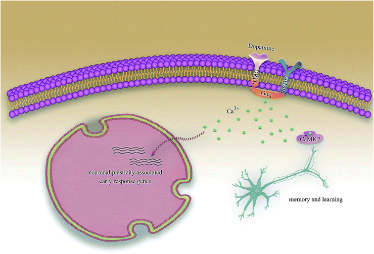
Alzheimer's disease (AD) is a progressive degenerative disease of the nervous system characterized by generalized dementia. The clinical symptoms include memory impairment, aphasia, dyslexia, visual spatial skills impairment, executive dysfunction, and personality and behavior changes. Although, so far, the mechanisms of AD are not completely clear and the existing drugs are effective only in alleviating symptoms and not cure them, it is already clear that early diagnosis and early therapy of AD play a significantly positive role in improving the prognosis of patients as well as reducing the disease burden. In addition, with the development of computer technology, computer-aided diagnosis and drug discovery has become one of the hottest research topics in the diagnosis and therapy of AD.1,2Hippocampal lesions have been considered as the early and defining pathology of AD;3 recent researches have demonstrated that growth hormone secretagogue receptor 1α (GHSR1α) and dopamine receptor D1 (DRD1), which are profusely co-expressed in the hippocampus, are involved in pathological processes.4,5 Activated GHSR1α could shift DRD1 from a Gαs to a Gαq state by forming GHSR1α/DRD1 heterodimers, then regulates DRD1-mediated initiating hippocampal synaptic reorganization via the non-canonical Gαq-Ca2+ signaling pathway, which results in the activation of Ca2+ dependent protein kinase II (CaMKII); the phosphorylation of CaMKII could activate the synaptic plasticity. However, a direct interaction of GHSR1α with β-amyloid (Aβ) in the hippocampus of patients with AD has been reported recently, which inhibited the activation of GHSR1α and prevented GHSR1α/DRD1 heterodimerization, leading to compromised GHSR1α regulation of DRD1 in the hippocampus of patients with AD. Several recent studies also show that the co-activation of GHSR1α/DRD1 protects GHSR1α from Aβ toxicity as well as prevents AD-mediated synaptic abnormalities and behavioral impairments in AD models.6,7 Even more interestingly, the new pathway has proved to be the cAMP-independent signaling pathway in the regulation of learning and memory, which is different from previous studies that have generally believed that AD is related to the cAMP signaling pathway.8 The proposal of the above studies provides a possible theoretical basis for the treatment of AD. We have been devoted to the computer-aided drug screening for many years.9 iScreen10 and iSMART11 were applied for virtual drug screening and computer-aided drug design. Traditional Chinese Medicine (TCM) is an independent theoretical system totally different from western medicine and has made encouraging achievements in the treatment of many diseases, especially chronic diseases, and has been applied widely. The TCM database12 has been applied to the development and promotion of TCM as well as the discovery of potential new drug. In addition, artificial intelligence technology has been greatly developed due to a substantial increase in the computing power, which has laid the foundation for the “hardware” and “software” of computer-aided drug design, protein–protein interaction, and the prediction of target proteins.13–15 Therefore, we can easily predict drug activity,16,17 perform molecular dynamics (MD) simulation experiments18,19 for small molecules, and predict the drug targets.20
2 Materials and methods
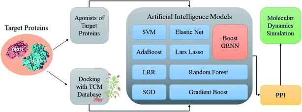
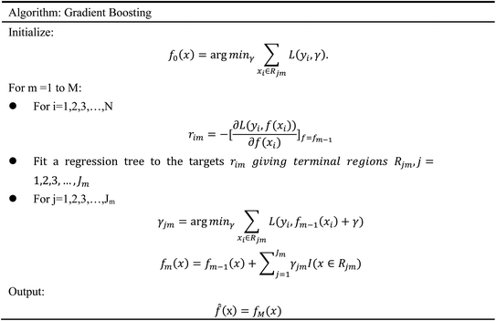
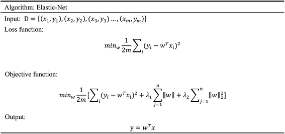
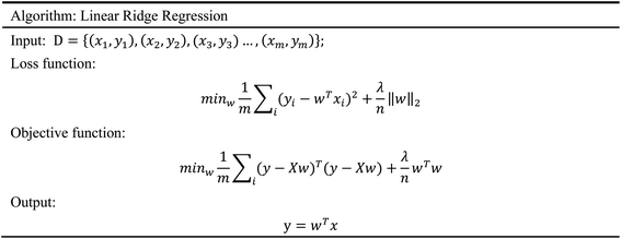
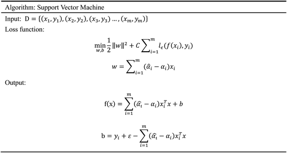
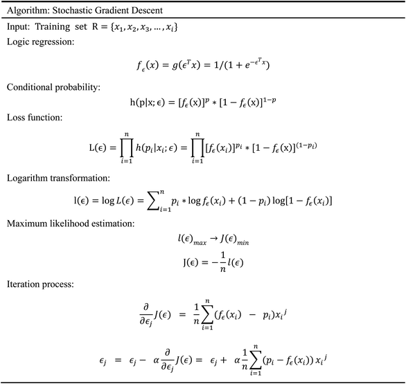
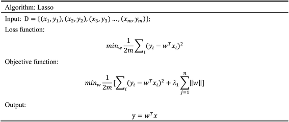
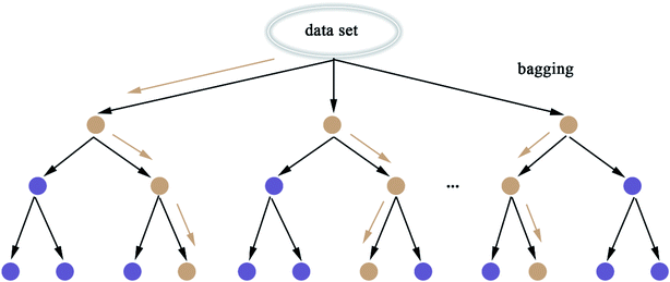
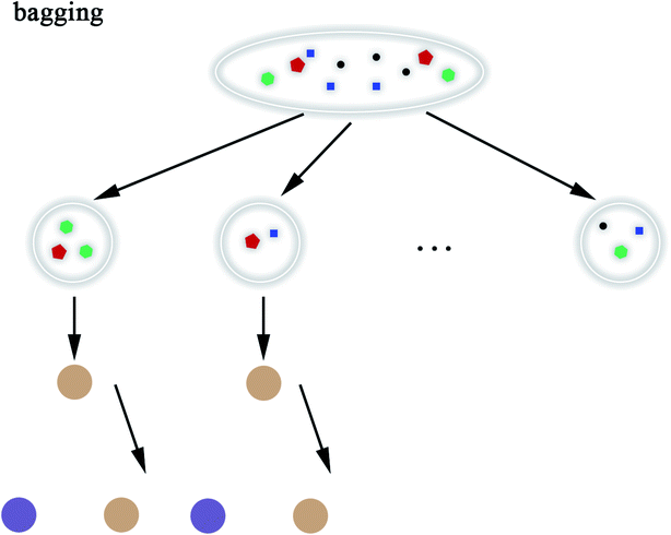
Accumulating evidence suggests that the lack of GHSR1α and DRD1 has a crucial role in the development of AD. Hence, in this paper, we chose nine artificial intelligent models to predict the drug activity for the new target proteins, which aims to identify the highest value of estimate binding affinity and the best docking score compounds from the TCM database that cloud activates the expressions of GHSR1α and DRD1 for the treatment of AD. In order to solve the problem of the overfitting of small data sets and incomplete properties of multi-feature data sets, we propose a novel boost Generalized Regression Neural Network (GRNN). A further experiment, MD, was performed to verify whether these candidate compounds obtained from virtual screening can bind to the target protein stably. The flow chart of the entire experiment is shown in Fig. 1.2.1 Network pharmacology analysis
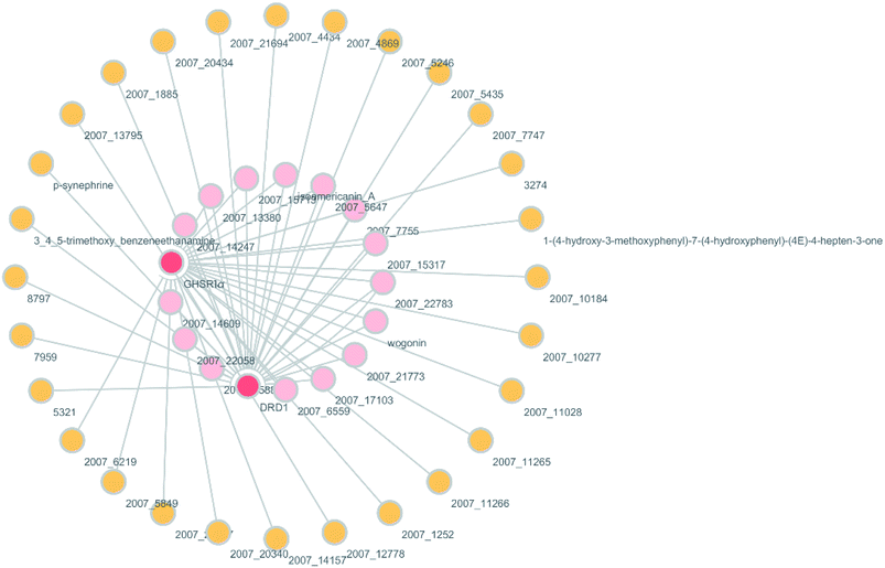
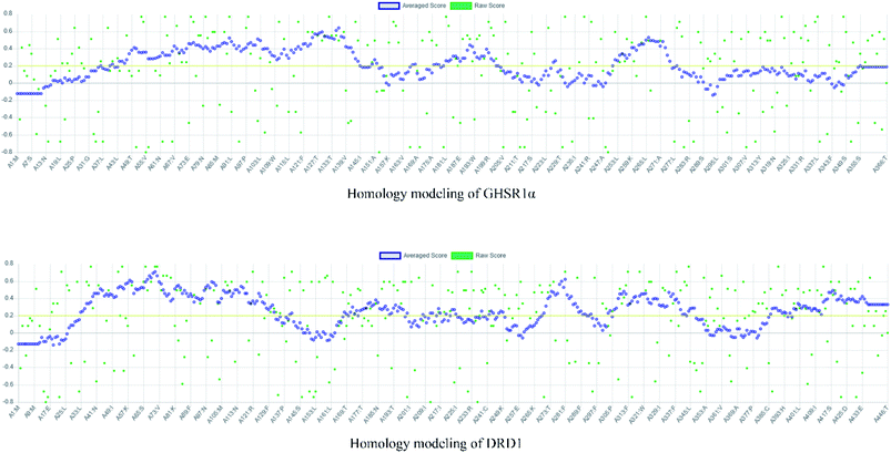
According to previous studies, we have determined that the target proteins are GHSR1α and DRD1; signal transmission depends on G Protein-Coupled Receptors (GPCRs), especially GHSR1α.4,6,7 Pathway data obtained from the novel research about AD and KEGG database21 was used to analyze the pathogenesis of AD, and the pathway diagram is shown in Fig. 2. GHSR1α and DRD1 were docked with the TCM database. The top 30 compounds from the TCM database with the dock scores were selected to draw the drug–protein interaction diagram by the Cytoscape software,22 which is shown in Fig. 3. Through the relevant research of the drug–protein interaction diagram, we are committed to finding out potential multi-target drugs that can interact with both GHSR1α and DRD1 at the same time.2.2 Screening and molecular docking
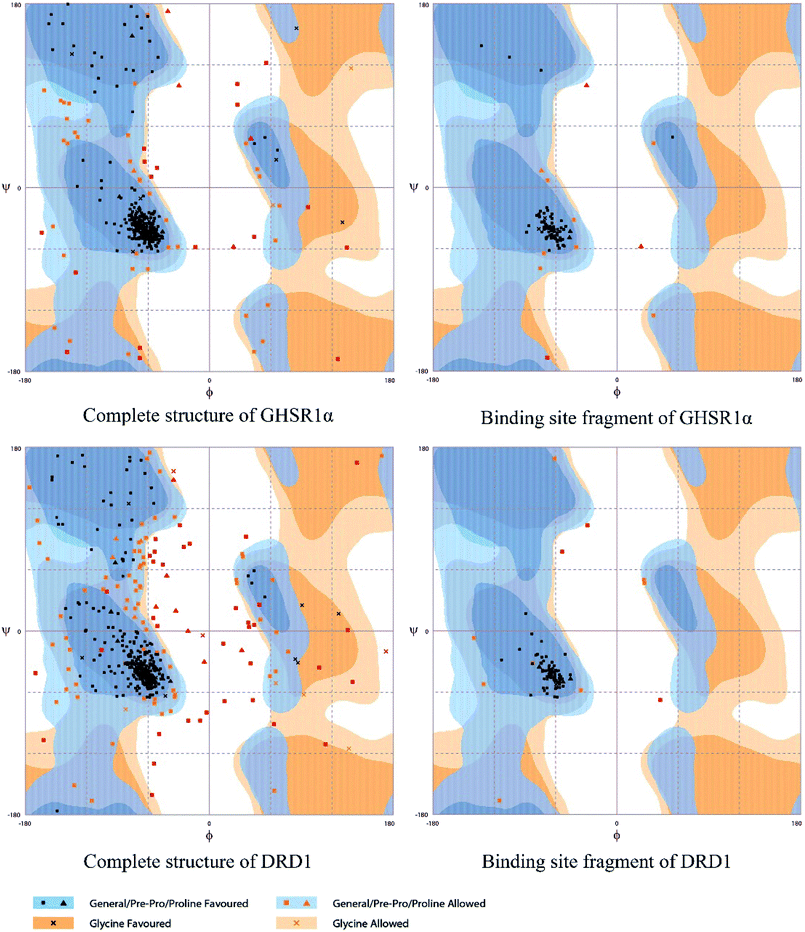
The crystal structures of DRD1 for AD were obtained from Protein Dara Bank (PDB ID: 1oz5).23 The protein sequences of GHSR1α and DRD1 were derived from Uniprot Knowledgebase (Uniprot ID: Q92847, Q6FH34).24,25 We input the protein sequence and crystal structure of different target proteins into I-Tasser26–29 for homology modeling. Through I-Tasser's modeling process, the complete protein crystal structures and ligands of the target proteins were obtained. In specific experimental operations, we selected the modeling structures with the highest stability and reliability for the next experiment. In order to judge whether the proteins 3D model obtained from I-Tasser are reliable, we drew the Ramachandran plot diagram and 3D-profile diagram for the target proteins, which are shown in Fig. 4 and 5, respectively.In order to make the target proteins more stable and reliable, the target proteins were removed from the crystal water and prepared by the Discovery Studio software (DS). At the same time, the ligands were used to define the binding sites of different target proteins. The TCM database,12 including 18![[thin space (1/6-em)]](https://www.rsc.org/images/entities/char_2009.gif) 776 small molecules of Chinese herbal medicine ingredients, has proved to be the best choice for molecular docking experiments.30,31 The ‘LigandFit module’32 was applied to dock the target proteins with the TCM database, which was included in the DS software. In our experiments, Chemistry at HARvard Macromolecular Mechanics (CHARMm27) was used to preprocess the target proteins, which could minimize the docking pose.33–35 For different targets, according to the results of molecular docking, we selected the top 30 compounds with the highest molecular docking score as the input data of the artificial intelligent models. ADMET descriptors module in DS include absorption, distribution, metabolism, excretion, toxicity, and other information, which were used to describe and comprehensively analyze the solubility, blood–brain barrier (BBB) penetration, hepatotoxicity, and cytochrome P450 2D6 (CYP2D6) of small molecules in the TCM database.36,37 In addition, SwissADME38 was used to judge whether the candidate compounds are the substrates of P-glycoprotein. According to the dock scores, ADMET descriptors results, and the predict results, we selected three possible candidates as the multi-target drugs for AD to perform the subsequent experiments.
776 small molecules of Chinese herbal medicine ingredients, has proved to be the best choice for molecular docking experiments.30,31 The ‘LigandFit module’32 was applied to dock the target proteins with the TCM database, which was included in the DS software. In our experiments, Chemistry at HARvard Macromolecular Mechanics (CHARMm27) was used to preprocess the target proteins, which could minimize the docking pose.33–35 For different targets, according to the results of molecular docking, we selected the top 30 compounds with the highest molecular docking score as the input data of the artificial intelligent models. ADMET descriptors module in DS include absorption, distribution, metabolism, excretion, toxicity, and other information, which were used to describe and comprehensively analyze the solubility, blood–brain barrier (BBB) penetration, hepatotoxicity, and cytochrome P450 2D6 (CYP2D6) of small molecules in the TCM database.36,37 In addition, SwissADME38 was used to judge whether the candidate compounds are the substrates of P-glycoprotein. According to the dock scores, ADMET descriptors results, and the predict results, we selected three possible candidates as the multi-target drugs for AD to perform the subsequent experiments.
2.3 Material and data preprocessing
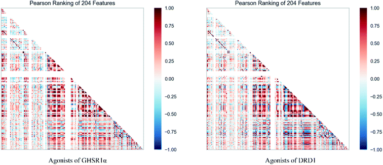
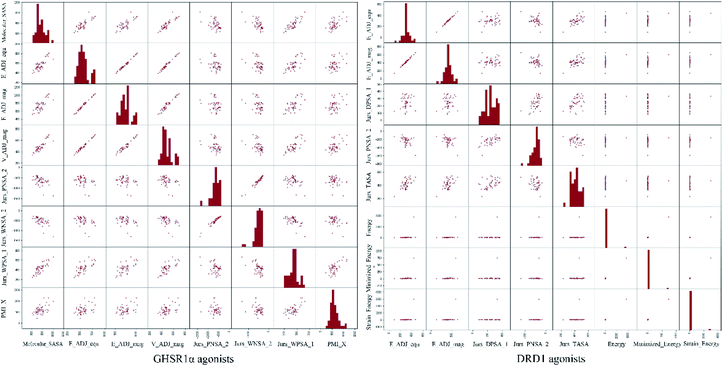
The agonists of the target proteins came from the ChEMBL database.39,40 We used these compounds to calculate the molecular properties. The number of these parameters describing molecular properties is as high as 204. During computer modeling, we selected the features so that the molecular features obtained can fit a more reasonable computer model. Excellent feature selection method is the basis to ensure the accuracy of the artificial intelligence models. We used Pearson correlation41 diagram to show the degree of correlation between each feature, which is shown in Fig. 6. Through this diagram, the relationship between each sample feature can be seen intuitively and it is clearly that there are quite a few molecular properties that are highly correlated with both the data sets of GHSR1α and DRD1. In order to show the relationship between the high-dimensional pairwise features more clearly, the scatter matrix diagrams were drawn based on the eight most relevant molecular properties. From the scatter matrix diagram, it can be clearly seen that there is a certain distribution correlation between each other of these molecular properties. The scatter matrix diagrams are shown in Fig. 7.2.4 Molecular dynamics simulation
In order to evaluate whether the candidates could become possible drugs more accurately, we choose to conduct MD simulation experiments. By analyzing the results of MD simulations, we could effectively analyze the stability of the compounds and the target proteins' binding. We used SwissParam web server to preprocess the candidates and generated the topology file, which provided a variety of information about the candidates including but not limited to atom type and bonding situation. Six 100 ns MD simulation experiments were implemented on the three candidates and two target proteins. The system temperature in NVT was set at 310 K for Maxwell distribution. Lincs constraint algorithm was adopted in these experiments to simulate the biological environment. Root mean square deviation (RMSD), total energy, the radius of gyrate, solvent-accessible solvent area (SASA), and root mean square deviation (RMSF) were used for the verification of the results of the MD simulation experiments.2.5 Artificial intelligence algorithms
3 Results and discussion
3.1 Network pharmacology analysis
A large number of previous studies have shown that the combined activation of GHSR1α and DRD1 is an effective treatment for AD.4,5,7,8 GHSR1α and DRD1 were considered as the target proteins for molecular docking with the TCM database. We selected the top 30 small molecule compounds ranked by the docking score in the docking results for network pharmacology analysis. The drug–protein interaction diagram is shown in Fig. 3. According to the results of network pharmacology analysis, we can easily understand that 15 small molecule compounds can simultaneously interact with GHSR1α and DRD1. These 15 compounds will be further analyzed to select the suitable candidates, which may be the possible drugs for AD.3.2 Virtual screening
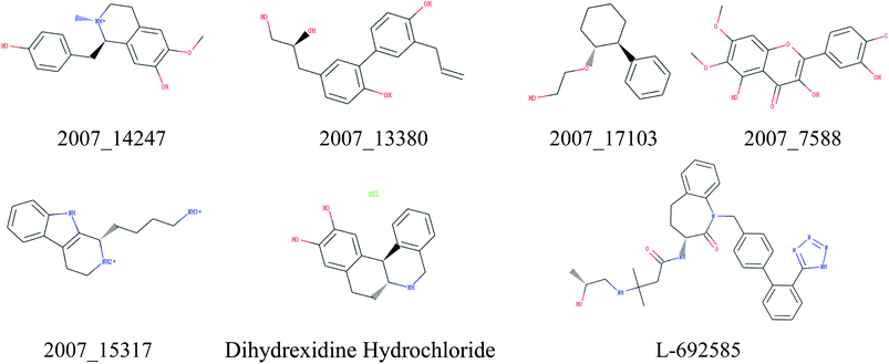
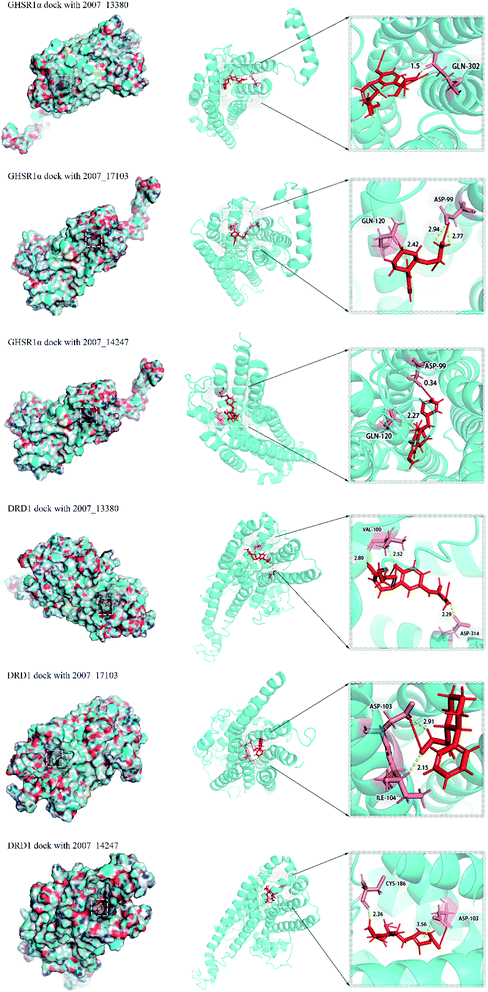
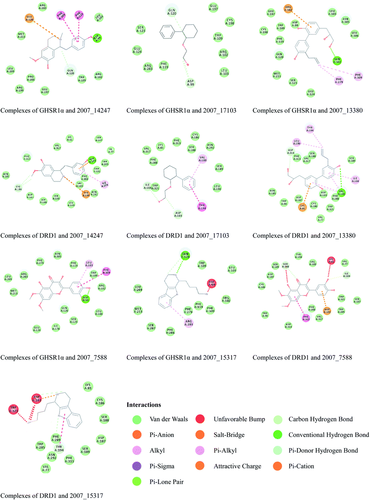
Through the drug–protein interaction diagram, we know that 15 compounds from TCM database can interact with two target proteins. However, through comprehensive analysis, we selected five compounds, namely, 2007_13380, 2007_17103, 2007_7588, 2007_15317, and 2007_14247, for the next experiment, which have a good affinity with both GHSR1α and DRD1. L-692585 (ref. 55) and dihydrexidine hydrochloride56 are the reference compounds of GHSR1α and DRD1, respectively. Compared with the reference compounds, the docking scores of the selected compounds are higher and the values of pEC50 are relatively close. The details of reference compounds are given in Table 1. The two-dimensional structures of the selected compounds and the reference compounds are given in Fig. 11. The docking results of the candidates are shown in Table 2 and Fig. 12. In order to evaluate the crystal structures of the target proteins, the 3D-profile diagrams were drawn. The results show that only a very small number of evaluation scores are less than 0, which means that our models are reasonable and reliable. Ramachandran plot was used to analyze whether the amino acid conformation is reasonable. The results show that almost all the conformation points fall within the allowable range. Ramachandran plots and 3D-profile diagrams are shown in Fig. 4 and 5, respectively. Finally, we choose 2007_14247, 2007_17103, and 2007_13380 as the candidate compounds. The complexes formed by these compounds from the TCM database and the target proteins are displayed in Fig. 13. 2007_14247 formed a carbon–hydrogen bond with GLN120 of GHSR1α at a distance of 2.27 Å and formed two carbon–hydrogen bonds with CYS186 of DRD1 at the same distance of 2.36 Å. 2007_17103 and GLN120 of GHSR1α formed a carbon–hydrogen bond with a distance of 2.42 Å and two carbon–hydrogen bonds with APS99; the distances are 2.94 Å and 2.77 Å, respectively. 2007_17103 and ILE104, APS103 of DRD1 formed two carbon–hydrogen bonds with a distance of 2.15 Å and 2.91 Å, respectively. 2007_13380 formed a hydrogen bond with GLN302 of GHSR1α at a distance of 1.5 Å and formed a hydrogen bond with VAL100 of DRD1 at a distance of 2.52 Å. 2007_15317 formed a 3.64 Å hydrogen bond with GHSR1α but at the same time, it also formed a bond with a strong adverse effect; the unfavorable bond length is 3.19 Å. Unfortunately, this compound forms three unfavorable bonds with DRD1. 2007_7588 and DRD1 formed two unfavorable bonds with GHSR1α. Therefore, we will not consider these two compounds from the TCM database in the later experiments. In order to more accurately determine whether the compounds are the effective Chinese medicine herbs for the treatment of AD, we used the ADMET descriptors37,57 to further evaluate these compounds. The results of ADMET descriptors are shown in Table 3. The parameter of absorption was used to evaluate the pure passive transport of compounds across the membrane. According to the results of the absorption level, 2007_14247, 2007_17103, 2007_13380, and 2007_15317 have excellent absorption. AlogP98 was used to evaluate the lipophilicity, which is an evaluation index for the hydrophilicity of these compounds. Drugs that require a central nervous system can bind to the target proteins only after passing the BBB. Comparing the BBB level evaluation values of these compounds, we believed that the penetration ability of 2007_7588 and 2007_15317 is poor. The indicator of CYP2D6 reflects whether these compounds have an inhibitory effect on the CYP2D6 enzyme. Among these compounds, only 2007_15317 has an inhibitory effect on the CYP2D6 enzyme. Hepatotoxicity was used to verify whether the compound has liver toxicity. The ADMET descriptor evaluation results shown that, except for 2007_17103 and 2007_15317, the other three compounds all have some hepatotoxic. The solubility parameter of the ADMET descriptors was used to express the solubility characteristics of these drugs. In order to verify the effectiveness of these compounds, we have to judge whether these compounds are the substrates of P-glycoprotein. According to the result, 2007_14247 and 2007_15317 are the substrates of P-glycoprotein. Considering the above factors, we selected 2007_13380, 2007_17103, and 2007_14247 as the possible compounds for the next experiment.| Name | Relationship | EC50 (nM) | pEC50 (nM) | Dock score |
|---|---|---|---|---|
| L-692585 | Reference compound of GHSR1α | 3 | 8.523 | 80.695 |
| Dihydrexidine hydrochloride | Reference compound of DRD1 | 72 | 7.143 | 68.67 |
| Name | Dock score of GHSR1α | Dock score of DRD1 |
|---|---|---|
| 2007_14247 | 121.472 | 114.392 |
| 2007_17103 | 108.997 | 114.699 |
| 2007_13380 | 114.163 | 110.554 |
| 2007_7588 | 133.836 | 113.422 |
| 2007_15317 | 129.466 | 108.701 |
| Name | Absorption | AlogP98 | BBB level | CYP2D6 | Hepatotoxicity | Log solubility | Substrate of P-glycoprotein |
|---|---|---|---|---|---|---|---|
| 2007_14247 | 0 | 1.85 | 2 | 0 | 1 | −2.342 | Yes |
| 2007_17103 | 0 | 2.72 | 1 | 0 | 0 | −2.838 | No |
| 2007_13380 | 0 | 3.078 | 2 | 0 | 1 | −2.244 | No |
| 2007_7588 | 1 | 1.84 | 4 | 0 | 1 | −3.185 | No |
| 2007_15317 | 0 | −0.017 | 3 | 1 | 0 | −0.333 | Yes |
3.3 Artificial intelligence algorithms analysis
| Name | Model | ||||||||
|---|---|---|---|---|---|---|---|---|---|
| AdaBoost | GB | EN | LRR | SVM | SGD | LL | RF | Boost GRNN | |
| 2007_14247 | 7.875 | 6.891 | 7.493 | 9.201 | 8.193 | 8.085 | 7.981 | 8.177 | 8.639 |
| 2007_17103 | 8.026 | 7.687 | 8.667 | 10.057 | 8.004 | 8.902 | 8.552 | 8.414 | 6.590 |
| 2007_13380 | 8.441 | 6.891 | 9.732 | 11.079 | 8.398 | 10.039 | 10.407 | 8.454 | 6.571 |
| 2007_7588 | 8.022 | 7.855 | 7.991 | 7.929 | 7.996 | 9.061 | 7.633 | 7.808 | 6.462 |
| 2007_15317 | 7.730 | 8.519 | 6.834 | 7.004 | 7.604 | 6.255 | 7.007 | 7.902 | 8.068 |
| Name | Model | ||||||||
|---|---|---|---|---|---|---|---|---|---|
| AdaBoost | GB | EN | LRR | SVM | SGD | LL | RF | Boost GRNN | |
| 2007_14247 | 8.695 | 8.353 | 9.002 | 8.434 | 8.342 | 8.778 | 8.747 | 8.543 | 7.878 |
| 2007_17103 | 7.704 | 7.172 | 8.021 | 8.416 | 8.044 | 7.632 | 7.618 | 7.997 | 7.097 |
| 2007_13380 | 7.490 | 7.713 | 7.629 | 7.489 | 7.625 | 7.602 | 7.671 | 7.501 | 7.007 |
| 2007_7588 | 7.818 | 7.936 | 8.382 | 7.541 | 7.773 | 8.206 | 8.380 | 7.997 | 7.097 |
| 2007_15317 | 9.194 | 7.978 | 8.312 | 8.650 | 7.916 | 8.214 | 8.478 | 8.929 | 7.007 |
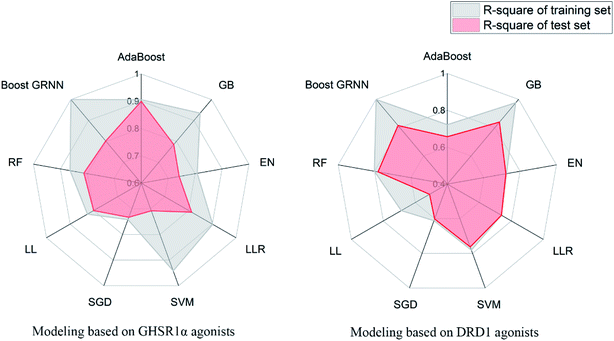
The model evaluation results are shown in Table 6. The visualized training results are shown in Fig. 14. According to this diagram, we can obviously see that compared to other models, our boost GRNN model has better accuracy and the R-square values of the training sets reached 0.8 or more for data sets of both GHSR1α and DRD1. Using artificial intelligence technology, we predict drug activity based on the features of the agonists of target proteins. In order to further explore the druggability of 2007_14247, 2007_17103, and 2007_13380, several MD experiments were performed to validate the stability of the protein-ligand complex.
| Model | GHSR1α | DRD1 | ||
|---|---|---|---|---|
| R2 of training set | R2 of test set | R2 of training set | R2 of test set | |
| AdaBoost | 0.906 | 0.900 | 0.722 | 0.657 |
| GB | 0.935 | 0.785 | 0.976 | 0.839 |
| EN | 0.808 | 0.741 | 0.725 | 0.722 |
| LRR | 0.902 | 0.813 | 0.738 | 0.738 |
| SVM | 0.942 | 0.708 | 0.781 | 0.763 |
| SGD | 0.742 | 0.733 | 0.611 | 0.601 |
| LL | 0.827 | 0.801 | 0.688 | 0.511 |
| RF | 0.864 | 0.813 | 0.801 | 0.781 |
| Boost GRNN | 0.999 | 0.802 | 0.999 | 0.815 |
3.4 Molecular dynamics simulation analysis
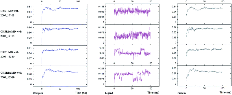
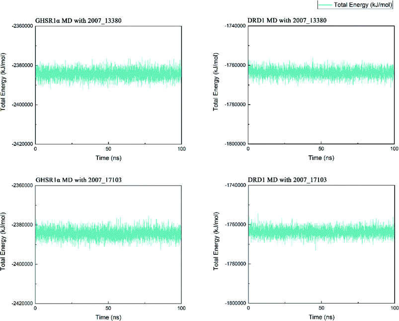
Three possible compounds that simultaneously interact with both GHSR1α and DRD1 were selected for the 100 ns MD simulation experiments. MD results showed that only 2007_13380 and 2007_17103 could stably interact with the two target proteins, while 2007_14247 completely deviated from GHSR1α during the process of MD. Therefore, the 2007_14247 cloud not interact with two target proteins stably. According to the results of RMSD analysis (Fig. 15), the RMSD curve of the complex formed by GHSR1α and 2007_13380 had an obvious upward trend in the range of 0–20 ns and had obvious fluctuations in the range of 0–35 ns. We considered that the fluctuations of the RMSD curve of the complex might be cause by the change in the conformation because of the ligand bound into the target protein. At about the same time, the same situation appeared on the RMSD curves of the complexes formed by DRD1 and 2007_13380, GHSR1α and 2007_17103, DRD1 and 2007_17103, respectively. Similarly, we considered that the same reason caused the same situation. Within 20–50 ns, there was a certain fluctuation in the RMSD curve of the complex composed of DRD1 and 2007_17103. It might be due to the change in the conformation of the complex after the ligand entered the target protein. However, fortunately, the RMSD curve returned to a calm and stable state after fluctuations. The RMSD curve of the complex formed by DRD1 and 2007_13380 almost showed a flat trend at 15–100 ns. These curves of the four complexes eventually showed a state of convergence. In the MD simulation experiments of GHSR1α, the RMSD of 2007_13380 fluctuated greatly, the RMSD curve of 2007_17103 was relatively stable and flat; in the MD simulation experiment of DRD1, the RMSD curve of 2007_13380 had a small fluctuation, and the curve of 2007_17103 was flat and stable. On the whole, compared to the RMSD curves of the complexes, the fluctuation of the RMSD curves of the ligands were negligible. The curves of the target proteins and the complexes had a great similarity; it can be shown that the target proteins have a larger effect of the overall RMSD curves trend. At the same time, we also analyzed the total energy of the four simulation experiments. The results showed that the total energy of the system in these MD simulation experiments were stable, which were maintained between −2![[thin space (1/6-em)]](https://www.rsc.org/images/entities/char_2009.gif) 390
390![[thin space (1/6-em)]](https://www.rsc.org/images/entities/char_2009.gif) 000 KJ mol−1 to −2
000 KJ mol−1 to −2![[thin space (1/6-em)]](https://www.rsc.org/images/entities/char_2009.gif) 380
380![[thin space (1/6-em)]](https://www.rsc.org/images/entities/char_2009.gif) 000 KJ mol−1, −1
000 KJ mol−1, −1![[thin space (1/6-em)]](https://www.rsc.org/images/entities/char_2009.gif) 777
777![[thin space (1/6-em)]](https://www.rsc.org/images/entities/char_2009.gif) 000 KJ mol−1 to −1
000 KJ mol−1 to −1![[thin space (1/6-em)]](https://www.rsc.org/images/entities/char_2009.gif) 760
760![[thin space (1/6-em)]](https://www.rsc.org/images/entities/char_2009.gif) 000 KJ mol−1, −2
000 KJ mol−1, −2![[thin space (1/6-em)]](https://www.rsc.org/images/entities/char_2009.gif) 390
390![[thin space (1/6-em)]](https://www.rsc.org/images/entities/char_2009.gif) 000 KJ mol−1 to −2
000 KJ mol−1 to −2![[thin space (1/6-em)]](https://www.rsc.org/images/entities/char_2009.gif) 380
380![[thin space (1/6-em)]](https://www.rsc.org/images/entities/char_2009.gif) 000 KJ mol−1 and −1
000 KJ mol−1 and −1![[thin space (1/6-em)]](https://www.rsc.org/images/entities/char_2009.gif) 777
777![[thin space (1/6-em)]](https://www.rsc.org/images/entities/char_2009.gif) 000 KJ mol−1 to −1
000 KJ mol−1 to −1![[thin space (1/6-em)]](https://www.rsc.org/images/entities/char_2009.gif) 760
760![[thin space (1/6-em)]](https://www.rsc.org/images/entities/char_2009.gif) 000 KJ mol−1, respectively. The diagrams of total energy are shown in Fig. 16.
000 KJ mol−1, respectively. The diagrams of total energy are shown in Fig. 16.
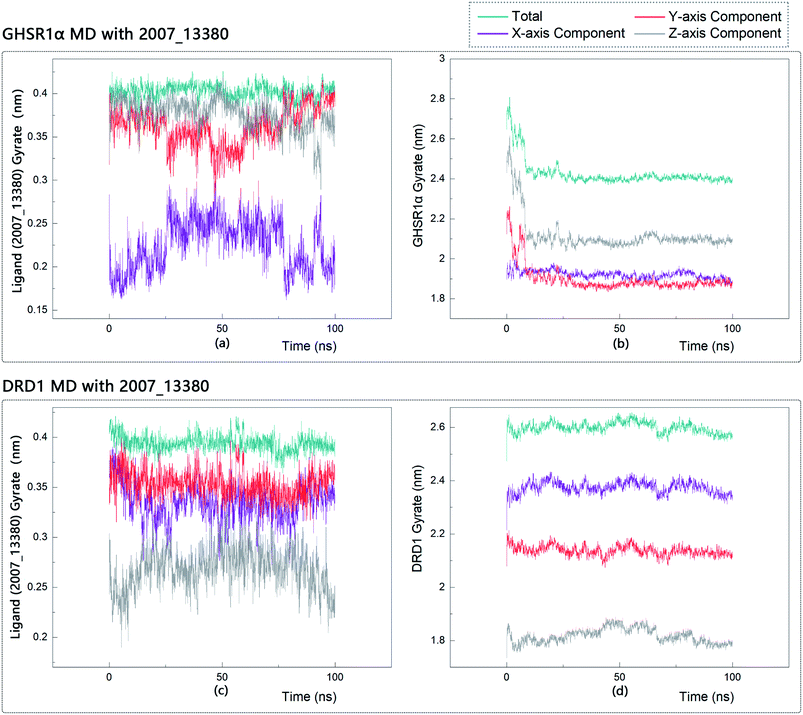
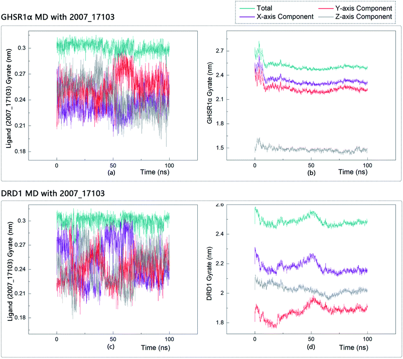
The radius of gyration reflects the volume and shape of the complex. The larger the radius of gyration, the more expansion of the complex. We calculated the gyration radius of the total, X axis, Y axis, and Z axis. From our experimental results of gyration, it could be seen that during 0–15 ns, the rotation rate of GHSR1α showed a rapid decline (Fig. 17b and 18b), which indicated that the GHSR1α protein structure was tightening rapidly during the process of MD simulation; the gyration curve of DRD1 was relatively flat in the experiment of DRD1 MD with 2007_13380 (Fig. 17d) while the DRD1 gyration curve has a great fluctuation in the experiment of DRD1 MD with 2007_17103 (Fig. 18d) during 0–65 ns. Fortunately, the curves tend to be stable in the range of 65–100 ns. In the range of 15–100 ns, the gyration curve of GHSR1α MD with 2007_13380 (Fig. 17b) tended to be flat; the gyration curve of GHSR1α MD with 2007_17103 (Fig. 18b) has a slight fluctuation close to flat. Ligands MD with GHSR1α, X axis, Y axis, and Z axis curves fluctuated greatly for both GHSR1α MD with 2007_13380 and GHSR1α MD with 2007_17103; fortunately, the decisive indicator total curves are nearly flat (Fig. 17a and 18a). In the experiment of DRD1 MD with 2007_13380, the gyration curves of 2007_13380 (Fig. 17c), total, X axis, and Y axis curves are relatively stable; however, the curve of Z axis has a certain range of fluctuations. In the experiment of DRD1 MD with 2007_17103, there existed fluctuations in the X axis, Y axis, and the Z axis (Fig. 18c), while the total curve tended to be flat. Generally speaking, although there are fluctuations of different amplitudes on the X axis, Y axis, and Z axis, the decisive indicator total components tend to be stable; thus, we have reason to believe that ligand binding in the protein is relatively stable.
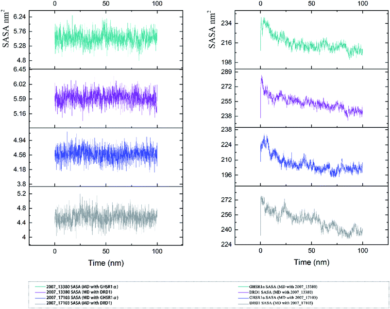
The SASA indicator helped us to judge the hydrophobicity of the protein and the state of the protein surface. We calculated the SASA data of the four MD experiments of GHSR1α and DRD1 (Fig. 19). The SASA results showed that the ligands were quite stable in these MD experiments and the SASA curves of the two target proteins dropped sharply at 0–50 ns. However, the SASA curves tends to be flat at 50–100 ns. The results of SASA further demonstrated that during the simulation timescale, the ligand–protein complexes formed by the target proteins and candidates are stable.
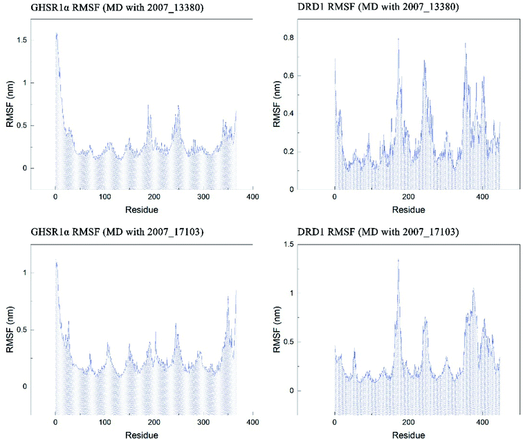
The RMSF indicator was used to evaluate the variation of each residue in these simulation experiments. The higher the RMSF value, the more unstable the residue is. In other words, the residue changed greatly before and after the simulation experiments. We calculated the RMSF values of the two target protein residues, as shown in Fig. 20. From the RMSF curve diagram, we could see that the GHSR1α residues behave well overall in the experiment of MD with 2007_13380 and there exist local residues with poor stability; residues in the range of 0–25 and 340–366 had higher RMSF values when MD with 2007_17103 was performed. For the MD simulation experiment of DRD1 and 2007_13380, there exist two ranges of 150–250 ns and 350–400 ns in which the stability of the residues was poor; the last picture of the RMSF curves showed that a small number of residues in the tail of DRD1 was unstable.
We superimposed these proteins obtained from the simulation experiments and used the RMSD indicator to evaluate these conformations. The conformations of GHSR1α and DRD1 before and after the experiment were superimposed, which are shown in Fig. 21. The RMSD of GHSR1α superposition structures reached 2.267 and 2.493 for the MD experiments of 2007_13380 and 2007_17103, respectively. The RMSD of DRD1 superposition structures reached 5.500 and 3.725 for the MD experiments of 2007_13380 and 2007_17103, respectively.
The superimposed results of the average structure and the final conformation obtained from the MD experiments are shown in Fig. 22. Both GHSR1α and DRD1 achieved good superposition results reaching 1.161 and 1.746, respectively, which indicate that these structures have great similarities.
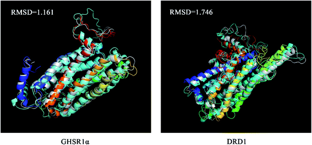 | ||
| Fig. 22 The average structure (silver) and the final state structure were superimposed to obtain the RMSD values. | ||
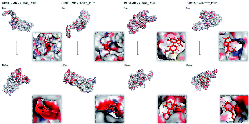
Finally, we drew the comparison diagram of the conformational changes of the complexes in the four MD experiments (Fig. 23). From the diagram, we can clearly see that all the ligands are still firmly bound to the target proteins in the protein at the end of the MD simulation experiments.
4 Conclusion
Overall, relying on the world's largest TCM database and the versatile artificial intelligence technology, we have found the Chinese medicine ingredients suitable for AD. The prediction results of artificial intelligent models show that 2007_14247, 2007_17103, 2007_13380, 2007_7588, and 2007_15317 have high drug activity. In order to verify whether the prediction results are reliable, we performed MD simulation experiments simulating 2007_14247, 2007_13380, and 2007_17103 with GHSR1α and DRD1. 2007_14247 was detached from GHSR1α. 2007_13380 and 2007_17103 still binds to the two target proteins stably. Therefore, we consider that 2007_13380 and 2007_17103 are the possible multi-target candidates for AD.Author contributions
Calvin Yu-Chian Chen designed research. Zi-Qiang Tang, Lu Zhao worked together to complete the experiment and analyzed the data. Calvin Yu-Chian Chen, Lu Zhao contributed to analytic tools. Zi-Qiang Tang, Lu Zhao, and Calvin Yu-Chian Chen wrote the manuscript together.Conflicts of interest
The author reports no conflicts of interest in this work.Acknowledgements
This work was supported by Guangzhou Science and Technology fund (Grant No. 201803010072), Science, Technology and Innovation Commission of Shenzhen Municipality (JCYL 20170818165305521) and China Medical University Hospital (DMR-110-097). We also acknowledge the start-up funding from SYSU “Hundred Talent Program”.References
- H. Parmar, B. Nutter, R. Long, S. Antani and S. Mitra, J. Med. Imaging, 2020, 7, 1–14 Search PubMed.
- S. Simpraga, R. Alvarez-Jimenez, H. D. Mansvelder, J. M. A. van Gerven, G. J. Groeneveld, S.-S. Poil and K. Linkenkaer-Hansen, Sci. Rep., 2017, 7, 5775 CrossRef.
- S. W. Scheff, D. A. Price, F. A. Schmitt and E. J. Mufson, Neurobiol. Aging, 2006, 27, 1372–1384 CrossRef CAS.
- J. Tian, L. Guo, S. Sui, C. Driskill, A. Phensy, Q. Wang, E. Gauba, J. M. Zigman, R. H. Swerdlow, S. Kroener and H. Du, Sci. Transl. Med., 2019, 11, eaav6278 CrossRef.
- G. Navarro, D. Aguinaga, E. Angelats, M. Medrano, E. Moreno, J. Mallol, A. Cortés, E. I. Canela, V. Casadó and P. J. McCormick, J. Biol. Chem., 2016, 291, 13048–13062 CrossRef CAS.
- A. Kern, M. Mavrikaki, C. Ullrich, R. Albarran-Zeckler, A. F. Brantley and R. G. Smith, Cell, 2015, 163, 1176–1190 CrossRef CAS.
- A. Kern, C. Grande and R. G. Smith, Front. Endocrinol., 2014, 5, 129 Search PubMed.
- T. Abel, P. V. Nguyen, M. Barad, T. A. Deuel, E. R. Kandel and R. J. C. Bourtchouladze, Cell, 1997, 88, 615–626 CrossRef CAS.
- Y.-C. Chen, Trends Pharmacol. Sci., 2015, 36, 78–95 CrossRef.
- T.-Y. Tsai, K.-W. Chang and C. Y.-C. Chen, J. Comput.-Aided Mol. Des., 2011, 25, 525–531 CrossRef CAS.
- K.-W. Chang, T.-Y. Tsai, K.-C. Chen, S.-C. Yang, H.-J. Huang, T.-T. Chang, M.-F. Sun, H.-Y. Chen, F.-J. Tsai and C. Y.-C. Chen, J. Biomol. Struct. Dyn., 2011, 29, 243–250 CrossRef CAS.
- C. Y.-C. Chen, PLoS One, 2011, 6, e15939 CrossRef CAS.
- M. Hassan Baig, K. Ahmad, S. Roy, J. Mohammad Ashraf, M. Adil, M. Haris Siddiqui, S. Khan, M. Amjad Kamal, I. Provazník and I. Choi, Curr. Pharm. Des., 2016, 22, 572–581 CrossRef.
- S. Ekins, A. C. Puhl, K. M. Zorn, T. R. Lane, D. P. Russo, J. J. Klein, A. J. Hickey and A. M. Clark, Nat. Mater., 2019, 18, 435–441 CrossRef CAS.
- X. Wang, B. Yu, A. Ma, C. Chen, B. Liu and Q. Ma, Bioinformatics, 2019, 35, 2395–2402 CrossRef CAS.
- E. Lounkine, M. J. Keiser, S. Whitebread, D. Mikhailov, J. Hamon, J. L. Jenkins, P. Lavan, E. Weber, A. K. Doak and S. Côté, Nature, 2012, 486, 361–367 CrossRef CAS.
- X. Yang, Y. Wang, R. Byrne, G. Schneider and S. Yang, Chem. Rev., 2019, 119, 10520–10594 CrossRef CAS.
- A. Khan, S. S. Ali, M. T. Khan, S. Saleem, A. Ali, M. Suleman, Z. Babar, A. Shafiq, M. Khan and D.-Q. Wei, J. Biomol. Struct. Dyn., 2020, 1–12 Search PubMed.
- S. A. Hollingsworth and R. O. Dror, Neuron, 2018, 99, 1129–1143 CrossRef CAS.
- G. Bitencourt-Ferreira, A. D. da Silva and W. F. de Azevedo, Curr. Med. Chem., 2020, 253–265 CrossRef.
- E. Altermann and T. R. Klaenhammer, BMC Genomics, 2005, 6, 60 CrossRef.
- P. Shannon, A. Markiel, O. Ozier, N. S. Baliga, J. T. Wang, D. Ramage, N. Amin, B. Schwikowski and T. Ideker, Genome Res., 2003, 13, 2498–2504 CrossRef CAS.
- R. K. Sunahara, H. B. Niznik, D. M. Weiner, T. M. Stormann, M. R. Brann, J. L. Kennedy, J. Gelernter, R. Rozmahel, Y. Yang and Y. Israel, Nature, 1990, 347, 80–83 CrossRef CAS.
- R. G. Smith, R. J. Leonard, A. R. T. Bailey, O. C. Palyha, S. D. Feighner, C. Tan, K. K. Mckee, S. Pong, P. R. Griffin and A. D. Howard, Endocrine, 2001, 14, 9–14 CrossRef CAS.
- R. Apweiler, A. M. Bairoch, C. H. Wu, W. C. Barker, B. Boeckmann, S. Ferro, E. Gasteiger, H. Huang, R. Lopez and M. Magrane, Nucleic Acids Res., 2004, 32, 115–119 CrossRef.
- J. Yang and Y. Zhang, Curr. Protoc. Bioinf., 2015, 52, 5.8.1–5.8.15 Search PubMed.
- J. Yang, R. Yan, A. Roy, D. Xu, J. Poisson and Y. Zhang, Nat. Methods, 2015, 12, 7–8 CrossRef CAS.
- W. Zheng, C. Zhang, E. W. Bell and Y. Zhang, Future Gener. Comput. Syst., 2019, 99, 73–85 CrossRef.
- J. Yang and Y. Zhang, Nucleic Acids Res., 2015, 43, W174–W181 CrossRef CAS.
- S. Thangapandian, S. John, S. Sakkiah and K. W. Lee, J. Chem. Inf. Model., 2011, 51, 33–44 CrossRef CAS.
- R. H. Khan, M. K. Siddiqi, V. N. Uversky and P. Salahuddin, Int. J. Biol. Macromol., 2019, 127, 250–270 CrossRef CAS.
- C. M. Venkatachalam, X. Jiang, T. Oldfield and M. Waldman, J. Mol. Graphics Modell., 2003, 21, 289–307 CrossRef CAS.
- K. Vanommeslaeghe, E. Hatcher, C. Acharya, S. Kundu, S. Zhong, J. Shim, E. Darian, O. Guvench, P. E. M. Lopes and I. Vorobyov, J. Comput. Chem., 2009, 31, 671–690 Search PubMed.
- B. R. Brooks, C. L. Brooks, A. D. Mackerell, L. Nilsson, R. J. Petrella, B. Roux, Y. Won, G. Archontis, C. Bartels and S. Boresch, J. Comput. Chem., 2009, 30, 1545–1614 CrossRef CAS.
- B. R. Brooks, R. E. Bruccoleri, B. D. Olafson, D. J. States, S. Swaminathan and M. Karplus, J. Comput. Chem., 1983, 4, 187–217 CrossRef CAS.
- A. Ghaleb, A. Aouidate, H. B. E. Ayouchia, M. Aarjane, H. Anane and S.-E. Stiriba, J. Biomol. Struct. Dyn., 2020, 1–11 CrossRef.
- H. van de Waterbeemd and E. Gifford, Nat. Rev. Drug Discovery, 2003, 2, 192–204 CrossRef CAS.
- A. Daina, O. Michielin and V. Zoete, Sci. Rep., 2017, 7, 42717 CrossRef.
- A. Gaulton, L. J. Bellis, A. P. Bento, J. Chambers, M. Davies, A. Hersey, Y. Light, S. McGlinchey, D. Michalovich and B. Al-Lazikani, Nucleic Acids Res., 2012, 40, D1100–D1107 CrossRef CAS.
- G. Papadatos, A. Gaulton, A. Hersey and J. P. Overington, J. Comput.-Aided Mol. Des., 2015, 29, 885–896 CrossRef CAS.
- P. Sedgwick, BMJ, 2012, 345, e4483 CrossRef.
- T. Hastie, S. Rosset, J. Zhu and H. Zou, Stat. Its Interface, 2009, 2, 349–360 CrossRef.
- L. Deng, W. Yang and H. Liu, Front. Genet., 2019, 10, 637 CrossRef CAS.
- J. Friedman, T. Hastie and R. Tibshirani, J. Stat. Softw., 2010, 33, 1 Search PubMed.
- A. Schneider, G. Hommel and M. Blettner, Dtsch. Arztebl. Int., 2010, 107, 776 Search PubMed.
- H. Asai, S. Tanaka and K. Uegima, IEEE Trans Syst Man Cybern Syst, 1982, 12, 903–907 Search PubMed.
- M. A. Hearst, S. T. Dumais, E. Osuna, J. Platt and B. Scholkopf, IEEE Intell. Syst., 1998, 13, 18–28 Search PubMed.
- A. J. Smola and B. Scholkopf, Stat. Comput., 2004, 14, 199–222 CrossRef.
- M. W. Huang, C. W. Chen, W. C. Lin, S. W. Ke and C. F. Tsai, PLoS One, 2017, 12, e0161501 CrossRef.
- B. Kuo, H. Ho, C. Li, C. Hung and J. S. Taur, IEEE J. Sel. Top. Appl. Earth Obs. Remote Sens., 2014, 7, 317–326 Search PubMed.
- L. Wang, Y. Yang, R. Min and S. Chakradhar, Neural Netw., 2017, 93, 219–229 CrossRef.
- C. Khanji, L. Lalonde, C. Bareil, M.-T. Lussier, S. Perreault and M. Schnitzer, Med. Care, 2019, 57, 63–72 CrossRef.
- A. Avdeef, ADMET DMPK, 2020, 8, 29–77 CrossRef.
- Y. Chtioui, S. Panigrahi and L. Francl, Chemom. Intell. Lab. Syst., 1999, 48, 47–58 CrossRef CAS.
- R. G. Smith, L. H. Van der Ploeg, A. D. Howard, S. D. Feighner, K. Cheng, G. J. Hickey, M. J. Wyvratt Jr, M. H. Fisher, R. P. Nargund and A. A. Patchett, Endocr. Rev., 1997, 18, 621–645 CrossRef CAS.
- M. M. Lewis, V. J. Watts, C. P. Lawler, D. E. Nichols and R. B. Mailman, J. Pharmacol. Exp. Ther., 1998, 286, 345–353 CAS.
- B. Bayel Secinti, G. Tatar and T. Taskin Tok, J. Biomol. Struct. Dyn., 2019, 37, 2457–2463 CrossRef CAS.
Footnotes |
| † Electronic supplementary information (ESI) available. See DOI: 10.1039/d0ra10077c |
| ‡ These authors contributed equally to this work. |
| This journal is © The Royal Society of Chemistry 2021 |

