A transfer learning approach for improved classification of carbon nanomaterials from TEM images

Abstract

The extensive use of carbon nanomaterials such as carbon nanotubes/nanofibers (CNTs/CNFs) in industrial settings has raised concerns over the potential health risks associated with occupational exposure to these materials. These exposures are commonly in the form of CNT/CNF-containing aerosols, resulting in a need for a reliable structure classification protocol to perform meaningful exposure assessments. However, airborne carbonaceous nanomaterials are very likely to form mixtures of individual nano-sized particles and micron-sized agglomerates with complex structures and irregular shapes, making structure identification and classification extremely difficult. While manual classification from transmission electron microscopy (TEM) images is widely used, it is time-consuming due to the lack of automation tools for structure identification. In the present study, we applied a convolutional neural network (CNN) based machine learning and computer vision method to recognize and classify airborne CNT/CNF particles from TEM images. We introduced a transfer learning approach to represent images by hypercolumn vectors, which were clustered via K-means and processed into a Vector of Locally Aggregated Descriptors (VLAD) representation to train a softmax classifier with the gradient boosting algorithm. This method achieved 90.9% accuracy on the classification of a 4-class dataset and 84.5% accuracy on a more complex 8-class dataset. The developed model established a framework to automatically detect and classify complex carbon nanostructures with potential applications that extend to the automated structural classification for other nanomaterials.

---

Introduction

Carbon nanomaterials such as carbon nanotubes/nanofibers (CNTs/CNFs) are an essential class of engineered nanomaterials (ENMs) for a wide range of industrial and scientific applications. As the global market expands from research and development to industrial high-volume production, there is an increasing concern over the safety and health risks associated with the occupational exposure to these materials.¹ Unlike other manufactured nanomaterials, CNT/CNF materials can have vastly different physical–chemical properties, depending on their synthesis methods and post-production treatments.^1,2 Recent epidemiology and toxicological studies for CNT/CNF suggest that tube/fiber dimensional characteristics, as well as the surface properties of agglomerates/bundles, are important determinants of their toxic effects.^1–3 Results from these studies indicate a need for improved particle identification, counting, and classification protocol to refine our ability to perform meaningful risk assessments for potential exposure to CNTs/CNFs. Transmission electron microscopy (TEM) imaging is a standard method for the size-specific measurement of nanomaterials. While TEM methods provide fundamental information for structural determination, manual classification of structures from TEM images is time-consuming and subject to operator bias—it depends on the operator's experience and background, and is restricted by the available time and resources. Many attempts were made to achieve automated identification and classification of airborne particles by combining analytical electron microscopy (AEM) imaging with the model-based classifier⁴ and artificial neural networks.^5,6 However, these classification models were primarily used to identify regular shapes of airborne particles rather than agglomerated fibrous structures. In contrast, CNT/CNF aerosols emitted in workplaces are often present in complex agglomerates mixed with fibrous structures;⁷ moreover, these agglomerates do not always possess readily identifiable morphologies, making it difficult to distinguish them from other non-fibrous/background particles by the conventional pattern recognition methods. To reduce bias and uncertainty by human classification and improve overall classification efficiency, there is a need for a robust method that can automate the recognition and classification of structures with high accuracy and computational efficiency.

In recent years, data scientists and materials researchers have proposed many innovative approaches utilizing artificial machine intelligence to understand materials microstructure properties.^8–16 By applying computer vision techniques to materials science image datasets, surface properties, phase distributions, and structural features of materials can be captured, measured with high precision, and quantified to investigate the underlying structure–properties relationship.¹⁷ These machine learning and computer vision methods often used supervised learning techniques such as Support Vector Machine (SVM)^9,10,13,14 and Convolutional Neural Network (CNN),^10,11 and unsupervised dimensionality reduction techniques such as t-distributed Stochastic Neighbor Embedding (t-SNE).^9–11 Machine learning algorithms make predictions on unseen data using the statistical models that were trained on previously collected data, by assuming that the distributions of the two data sets are the same.¹⁸ Since the first introduction of the ImageNet Large-Scale Visual Recognition Challenge (ILSVRC)¹⁹ and AlexNet²⁰ with a CNN framework,^21–24 numerous attempts have been made to construct high-performance architectures for image classification, single-object localization, and object detection. More recently, data-driven machine learning models have been successfully applied to classify experimental images of nanomaterials such as graphene,²⁵ metallic nanoparticles,²⁶ and colloidal nanoparticles.²⁷

In this work, we used a dataset consisting of 5323 greyscale TEM images of various nanostructured carbon samples collected by the National Institute for Occupational Safety and Health (NIOSH). The dataset was split into a training set (80% of the dataset) to train the machine learning model, and a validation set (remaining 20% of the dataset) to evaluate the model performance via the 5-fold cross-validation method. To achieve the desired classification performance, we applied a deep CNN based supervised learning model with unsupervised embedding algorithms to the TEM image dataset for feature representation and structure classification.

Dataset and methods

TEM image dataset

Airborne samples containing carbon nanomaterials were collected on three-piece cassettes with mixed cellulose ester (MCE) filters, processed under the guidance of the modified NIOSH 7402 method and analyzed by a TEM for structure determination and classification.^1,2 The dataset consists of 5323 greyscale bright field images that covered all major types of airborne carbon nanostructures in workplaces during the manufacturing operations and handling of CNT/CNF materials. Structural classification based on these TEM images can provide useful information to assist the risk assessment for occupational exposure to these materials.

The hybridizations in electronic structures of carbon atoms allow them to constitute various carbon nanostructures with distinctive functionality.^28,29 CNT/CNFs are distinguishable from other carbonaceous nanomaterials by their unique fibrous and multi-layered structures.^29,30 Considering the native structures of CNT/CNFs and other alternative structural forms observed in the field samples, we specifically defined five major classes representing the most commonly seen CNT/CNF structures: Cluster (Cl), Fiber (Fi), Matrix (Ma), Matrix-Surface (MS) and Non-CNT (NC) as shown in Fig. 1, respectively. By definition, cylindrical carbon nanostructures with various stacking arrangements of graphene sheets and aspect ratios greater than 3 : 1 are classified as CNT/CNF fibers (Fi). A bundle of such fibers can form a cluster (Cl) where similar fibers are loosely contacted. It is known that CNT/CNFs aggregate easily due to the presence of inter-fiber interaction and their high level of flexibility.²⁸ For air samples collected in workplaces, CNT/CNF particles are most likely to aggregate and pack into a condensed matrix (Ma) structure. CNT/CNF fibers can be also found in large particles comprised of other carbonaceous materials, catalytic particles, and intermediate product particles emitted during the manufacturing and/or mixing operations of CNT/CNF materials. These mixed structures were especially examined at higher magnifications to verify the presence of extruded tube/fiber structures from their surfaces and classified as matrix-surface (MS). The remaining undefined structures were categorized as non-CNT (NC) structures, consisting of other carbonaceous materials such as graphene and soot, and environmental particles containing metals, minerals, and polymer contents.

Fig. 1 TEM images showing the pre-labeled major classes from the full dataset (columns a–e): (a) clusters (Cl) formed by loosely packed fibers, (b) single fibers (Fi), (c) condensed matrix (Ma) structures with embedded CNT/CNFs, (d) oversized mixed structures with CNT/CNFs on surfaces (MS), and (e) non-CNT structures (NC).

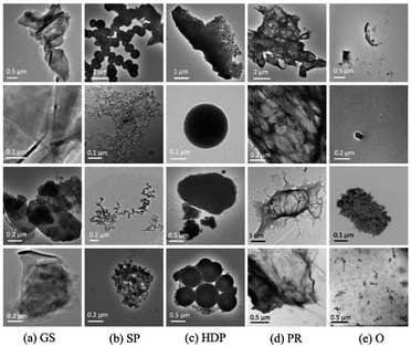
Considering the diverse particle types and morphologies in the NC class, we further classified the 1195 NC images, based on their shapes and edge characteristics, into five mini-classes (see Fig. 2): Graphene Sheets (GS), Soot Particles (SP), High-Density Particles (HDP), Polymer Residuals (PR), and Others (O). Graphene sheets are two-dimensional planar structures formed by sp² hybridized carbon atoms, represented by the layered structure and well-defined edges in TEM images.²⁸ Soot particles are typically fractal hydrophobic aggregates consisting of black carbon spherules with diameters in the range of 20–40 nm.³¹ High-density particles referred to metal or mineral particles with distinctive stacking patterns due to their closely packed crystalline structures. Polymer residues are segments of polymeric materials showing continuous and porous structures. The rest of the non-distinguishable structures were all grouped as others.

Fig. 2 TEM images showing representative structures of five sub-groups of the NC class (columns a–e): (a) overlapped multi-layer graphene sheets (GS), (b) aggregated soot particles (SP), (c) mineral or metal particles with high densities (HDP), (d) polymer residual fragments from the sampling environment (PR), (e) other particulates with the undetermined composition and morphologies (O).

The images in this dataset were manually identified, sorted into groups, pre-labeled, and cropped to match the size (224 × 224 pixels) required for the computational models. The distribution of pre-labeled images in the major classes and sub-groups of the NC class is illustrated in Fig. 3. These TEM images were taken under various magnifications to capture the entire particles as well as the specific surface structures. Because of the nature of samples, the size of features was not considered as important as the morphological properties for classification. Therefore, images were processed and highlighted on edge features but not on size information. Based on highly condensed vectorized edge information, the models can predict classifications for images taken at different magnification conditions.

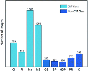Fig. 3 The number distribution of pre-labeled images in the CNT classes (Cl, Fi, Ma, MS) and sub-groups of the NC class (GS, SP, HDP, PR, and O).

Classification model

We constructed an image classification pipeline (Fig. 4) to include the following steps: (1) image pre-processing, (2) transfer learning using a pre-trained deep CNN, (3) hypercolumns as pixel descriptors³² to extract information from each pixel at different length scales, (4) Vector of Locally Aggregated Descriptors (VLAD) encoding and K-means clustering to classify the particle types, and (5) visualization and analysis of results. Each component is described in the following sections.

Fig. 4 A schematic of the image classification model: (1) blue arrows indicate the conventional image classification pipeline with a linear-softmax classifier (VGG16 + LS); (2) red arrows indicate the hypercolumn (Hcol) model followed by VLAD classifiers. In our model, pre-processed images were imported to the pre-trained CNN architecture as input, followed by the hypercolumn feature extraction. A K-means library was then used as a visual feature dictionary and introduced to a VLAD encoder to compute the residuals. Finally, the classifier was trained with a boosting cycle to make predictions.

Image pre-processing. The purpose of image pre-processing is to mitigate the imbalanced distribution of input data among different classified structures. As illustrated in Fig. 3, the Fi class only contributes about 8% of the total number of labeled images, compared to Ma's 32% and MS's 24%. Since the penalty for misclassifying the minority images as the majority images is smaller than that of the reverse error,³³ we applied a data augmentation technique to create additional artificial training images by modifying the original images. This approach³³ has been successfully applied in many computer vision tasks to overcome the issues associated with the deficient or imbalanced dataset.^34,35

Artificial augmentation can be achieved by either affine transformations (translation, shearing, rotation) or elastic distortions.³⁶ In this work, we applied 90 degree rotation transformations to the small size datasets (Cl, Fi, and mini-classes in NC) to add three times more images from the original images. By rotating the image, the pixels are completely rearranged while the structural features in the image are preserved. Therefore, artificial micrographs made by rotations can represent the real data for the images. Examples of original and corresponding augmented images with the affine transformation (normalized to 224 × 224 pixels) are shown in Fig. 5. To prevent the potential bias introduced by overfitting the large groups, we only augmented minor groups for the imbalanced dataset and mixed them with un-augmented major groups to create evenly distributed classes.

Fig. 5 Data augmentation with the affine transformation (90 degree rotation) on an image from the Cl class: (a) original image and (b–d) corresponding augmented images.

Transfer learning. A conventional CNN architecture requires a large training dataset (on the order of millions of images) to achieve the desirable prediction accuracy. Just like humans can parse unfamiliar images, CNNs trained from natural image datasets can be transferred to perform tasks on unseen image types. The rationale is that these deep neural networks can learn visual features that apply to a wide range of image types. Thus, we utilize a transfer learning approach based on the VGG-16 (ref. 21) CNN pre-trained with weights learned from the ILSVRC.^19,20

Hypercolumn representation. Selecting a representation scheme for images is a critical step for successful transfer learning. We tested two approaches: (1) a conventional CNN where the fully-connected (FC) layer is used in a linear softmax (LS) classifier, as shown by the blue arrows in Fig. 4, and (2) a hypercolumn (Hcol) feature representation that collects information at multiple length scales, as seen in the red arrows in Fig. 4. As illustrated in Fig. 6, the VGG-16 architecture consists of five convolutional (Conv) blocks and one FC classifier block. Each Conv block contains multiple Conv layers for pattern processing and a single Maxpooling layer for image size reduction. The FC classifier block has a flatten layer at the top for transforming 3-dimensional tensor to 1-dimensional long vector, followed by two FC layers and a softmax layer that enables certain controlled categories or classes as output.

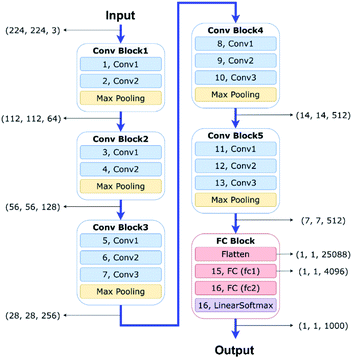Fig. 6 A schematic of our VGG-16 Deep Convolutional Neural Network (DCNN) architecture adapted from ref. 8 with permission from Elsevier.

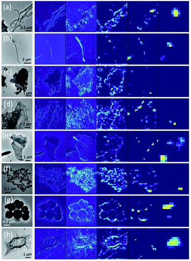
The feature vector produced by a conventional CNN only contains the large length scale information generated from the deepest layer of the network. In contrast, a hypercolumn is a vector that captures all network information at multiple length scales for a given pixel in the input image.³² A hypercolumn vector concatenates selected Conv layer activations and aggregates information from the various Conv blocks. For our model, we extracted 5 convolution layers (2, 4, 6, 9, and 12, as shown in Fig. 6) as the hypercolumn representation. Fig. 7 shows examples of Conv layer activations for the various hypercolumn components from 8 categories in our dataset. The length of the hypercolumn vector is the sum of the length scale for these layers, representing 1472 features per pixel. A full density hypercolumn of a 224 × 224 image can cover over 73 million features in the image. In contrast to the conventional transfer learning where the FC layer contains only 4096 features per image, the large number of features represented in the hypercolumn model enables a better coverage on different levels of information in the image. Instead of using a memory-intensive full density hypercolumn approach, we chose a fraction of the pixels at random in each image to be represented by the hypercolumns. Since the hypercolumn density had little impact on the classification performance in a range from 5% to 60%, we used a frugal hypercolumn density of 10%. The hypercolumn density is defined as the fraction of pixels that are used to create the hypercolumn representation.

Fig. 7 Examples of hypercolumn representations for eight image classes (a) Cl, (b) Fi, (c) Ma, (d) MS, (e) GS, (f) SP, (g) HDP, and (h) PR. Columns from left to right: original, hypercolumn representations for b1c2, b2c2, b3c2, b4c3, and b5c3 layers.

Machine learning pipeline. Using the hypercolumn feature vectors to perform classification of images includes three steps: (1) construction of a K-means library: use K-means³⁷ to cluster the feature vectors in the high-dimensional space, and represent visual features in K values by cluster centroids; (2) calculation of the residuals: calculate the residuals for local features relative to the closest cluster centroids³⁸ and concatenate the residuals to create the VLAD^38–40 as a compact representation for the image as a whole; (3) classification: construct a weak classifier by minimizing the residuals to reduce the differences between local features encoded in the VLAD vector and the visual dictionary cluster centroid. We proposed a boosting ensemble meta-algorithm to perform learning and tuning on the weak classifier to build a robust classifier.

In the machine learning pipeline, the hypercolumn representations are clustered via K-means, and the vector of cluster residuals characterizes the image as a whole. Thus, the number of clusters K is an important user-defined variable that can affect the overall classification performance. The selection of K in our model was based on practical considerations as discussed in the ESI S1.† We tested three types of boosting algorithms (AdaBoost,⁴¹ random forest,⁴² and gradient boosting^43,44) for classification performance. The effects of K on classification accuracy were evaluated for each boosting algorithm in the range 10 ≤ K ≤ 300. For all three methods, K had little impact on the classification accuracy above a threshold where K = 50. The testing results (see ESI Fig. S1†) shows that gradient boosting outperformed other algorithms in almost all of the classification tasks. Because the training time for gradient boosting increased significantly with K (see ESI Fig. S2†), we chose gradient boosting with K = 50 to build our classifier to achieve the optimal accuracy within reasonable computational time.

This methodology was initially proposed by DeCost¹⁰ and Kitahara¹¹ for microstructure cluster classification and analysis. One advantage of using VLAD encoding on convolution features is that it yields a deep representation of the image structure with no explicit high-level spatial dependence,⁴⁵ which is beneficial for a small size dataset. Additionally, the VLAD encoder is convenient for generalizing different hypercolumns from multiple layers with different characteristic length scales.

Data visualization. Visualizing the features represented by the VLAD encoder in a high dimensional space was realized by using the t-distributed stochastic neighbor embedding (t-SNE),^46–48 a dimensionality reduction technique that maps high dimensional data to two dimensions. It should be noted that because t-SNE maps a high-dimensional space into 2D, the diagram only indicates the similarities among different classes for comparison, but not in precise data projections. In this work, principal component analysis (PCA)⁴⁹ was used to project high dimensional image features described by VLAD encoding into a 2D representation. The results were then processed by t-SNE to calculate the pairwise distance for exploration.

Results and discussion

We applied the transfer learning methods to perform classification tasks on the 4-class CNT dataset (including Cl, Fi, Ma, and MS) and the 8-class full dataset (including Cl, Fi, Ma, MS, GS, SP, HDP, and PR). The comparison in Fig. 8 shows the average 5-fold cross-validation classification accuracy among 4 major classes when applying different transfer learning methods (linear softmax vs. hypercolumn with 10% density) and image pre-processing technique (original vs. augmented). The comparison was also performed for the 8-class full dataset as seen in Fig. 9. The detailed information on the classification accuracy for each class can be found in ESI Table S1.† A noticeable decrease in the total classification accuracy occurred when the dataset was extended from four to eight classes as the computed intermediate parameters increased from 4096 to over 73 000 000. We also note that the hypercolumn method achieved better classification performance than linear softmax for almost every particle class regardless of other factors. This is expected since the hypercolumn representation can capture more visual features at multiple length scales than conventional methods.

Fig. 8 Grid plots showing the classification accuracy for the 4-class dataset by applying different transfer learning models (shown in columns), and image pre-processing methods (shown in rows). Left column: conventional CNN model with a linear softmax classifier (VGG16 + LS); right column: hypercolumn-based approach (VGG16 + 10% Hcol); upper row: original, unbalanced dataset; lower row: augmented dataset after image pre-processing.

Fig. 9 Grid plots showing the classification accuracy for the 8-class dataset obtained by applying different transfer learning methods (shown in columns: VGG16 + LS vs. VGG16 + 10% Hcol), and image pre-processing method (shown in rows: original vs. augmented).

For the original image dataset (first rows in Fig. 8 and 9), the classification performance was affected by the size of the training set. CNT classes trained from the large image sets (1702 images for Ma, and 1259 images for MS) can be classified more accurately than other classes. The average classification accuracy ranges from about 50% to over 70% for the rest of the classes trained by the small datasets. We attribute this trend to the imbalanced image dataset. It was less costly for the model to misclassify rare image types, so the training method was biased to reward correct classification of frequently seen image classes.

To correct this bias, we created artificial images to supplement the rare image classes by using the data augmentation technique. The augmented dataset contained a total of 4800 images, evenly distributed among the eight image categories. Each category included 480 training and 120 validation images. This balanced dataset effectively improved the overall performance by increasing the total accuracy in almost every category for both the 4-class and 8-class datasets; it also decreased the variations in per-class accuracy, as evidenced by the smaller standard deviations in total accuracy as seen in Fig. 8 and 9. Once the augmentation was implemented, the classification performance was significantly improved for rare image types in both linear softmax and hypercolumn models.

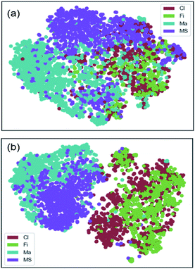
The effect of data augmentation can also be viewed in the t-SNE plots (see Fig. 10) showing the visual clustering of the image representations in the 4-class dataset. In these plots, each dot represents an image and is colored by the associated class membership. For the original data set as seen in Fig. 10(a), the plot shows prominent clusters of the major categories (Ma and MS) whereas very little separation among image sets. For the augmented data set as seen in Fig. 10(b), the plot shows two separate clusters corresponding to the fibrous structures (Cl and Fi) and the agglomerated structures (Ma and MS). Within those larger clusters, the individual classes can be resolved further as distinct sub-clusters. The enhanced clustering effect was a result of the improved classification in the balanced dataset.

Fig. 10 t-SNE representation showing the effects of data augmentation on the classification results for the 4-class set using the 10% Hcol transfer learning model: (a) original unbalanced dataset; (b) augmented and balanced dataset.

Confusion matrices were used to visualize how well the algorithm was performing classification tasks. Fig. 11 shows the true and predicted labels of the data for each class studied. As shown in Fig. 11, classification accuracies in the diagonal directions of matrices are very high. This indicates that the hypercolumn image representation using the augmented dataset gave the best classification results for both the 4- and 8-class datasets. For the 4-class dataset, overall classification accuracy was 90.9%, with per-class accuracy ranging from 89.1 to 92.4%. For the 8-class dataset, overall classification accuracy was 84.5%, with per-class accuracy ranging from 71.0 to 90.3%. Note that images from classes with high similarities (e.g., MS and Ma classes as shown in ESI Fig. S3†) are difficult to be correctly classified since the model treats all output classes equally. The misclassification rates of these classes can be seen in Fig. 11(a): 9% of true MS images were misclassified as Ma, whereas only 1% of them were falsely predicted as Cl or Fi class. Therefore, future work (discussed in ESI S3†) will focus on the design of a non-linear classifier to reduce such errors at the output stages. Also, improvements can be made by reconstructing a hierarchal workflow to better represent the image features.

Fig. 11 The performance of VGG16 + 10% Hcol model with the augmented dataset for (a) 4-class and (b) 8-class sets, presented as the confusion matrices. The vertical axis indicates the true class of an image, and the horizontal axis represents the predicted class.

Conclusion

In this work, we applied computer vision and machine learning tools to classify a dataset of TEM images of nanostructured carbon samples. We employed a transfer learning approach by using an existing state-of-art deep CNN architecture (VGG-16) trained from a large dataset of natural images (ImageNet) to build our classifiers. The images were represented by the hypercolumn vectors, which were clustered via K-means, processed into a VLAD representation, and used to train a softmax classifier with the gradient boosting algorithm. Our work suggests that hypercolumn feature representations provide significant improvement of classification accuracy when comparing to the traditional CNN models. Image augmentation can be an effective way to mitigate classification bias due to the presence of imbalanced datasets. This method achieved an overall 90.9% accuracy on the classification of a 4-class dataset and 84.5% accuracy on a more complex 8-class dataset. By analyzing the misclassified images, it shows that even the best performance model (VGG16 + 10% Hcol) has difficulties to distinguish images from classes with high similarities (i.e., matrix structures from MS and Ma classes, or fibrous structures from Cl and Fi classes). Optimization of the classifiers and application of a multi-stage classification workflow are both considered as future directions to reduce such errors during classification. This work thus presents a new machine learning approach to classify complex nanoscale structures from electron images for the determination of structure-related properties of carbon nanomaterials. The classification framework and data augmentation method can be adapted to applications aiming to classify irregular shaped structures as well as novel nanostructured materials such as 2D nanomaterials. Future efforts will focus on the development of a generalized modeling framework for classifying and analyzing images of other emerging nanomaterials.

Code availability

The source code for this work is available at the software code repository (https://github.com/NEML/ML-CNT).

Conflicts of interest

The findings and conclusions in this report are those of the authors and do not necessarily represent the views of the National Institute for Occupational Safety and Health. Mention of product or company name does not constitute endorsement by the Centers for Disease Control and Prevention.

Acknowledgements

We gratefully acknowledge funding for this work through the Nanotechnology Research Center (NTRC) of the National Institute for Occupational Safety and Health (NIOSH) (NTRC-9390BTM). This work was also supported by the National Science Foundation under award CMMI-1826218. We also greatly appreciate the important open-source Python libraries Keras⁵⁰ and Scikit-Learn⁵¹ for supporting our implementation and work.

References

1. NIOSH, Current Intelligence Bulletin 65: Occupational Exposure to Carbon Nanotubes and Nanofibers, DHHS (NIOSH), Publication No. 2013-145, Cincinnati, OH, 2013.
2. M. E. Birch, C. Wang, J. E. Fernback, H. A. Feng, Q. T. Birch and A. Dozier, Analysis of Carbon Nanotubes and Nanofibers on Mixed Cellulose Ester Filters by Transmission Electron Microscopy, NIOSH Manual of Analytical Methods, Cincinnati, OH, 5th edn, 2017.
3. G. Oberdörster, V. Castranova, B. Asgharian and P. Sayre, J. Toxicol. Environ. Health, Part B, 2015, 18, 121–212.
4. M. F. Meier, T. Mildenberger, R. Locher, J. Rausch, T. Zünd, C. Neururer, A. Ruckstuhl and B. Grobéty, J. Aerosol Sci., 2018, 123, 1–16.
5. D. Wienke, Y. Xie and P. K. Hopke, Anal. Chim. Acta, 1995, 310, 1–14.
6. Y. Xie, P. K. Hopke and D. Wienke, Environ. Sci. Technol., 1994, 28, 1921–1928.
7. M. M. Dahm, M. K. Schubauer-Berigan, D. E. Evans, M. E. Birch, J. E. Fernback and J. A. Deddens, Ann. Occup. Hyg., 2015, 59, 705–723.
8. K. Gopalakrishnan, S. K. Khaitan, A. Choudhary and A. Agrawal, Constr. Build. Mater., 2017, 157, 322–330.
9. B. L. DeCost and E. A. Holm, Comput. Mater. Sci., 2015, 110, 126–133.
10. B. L. DeCost, T. Francis and E. A. Holm, Acta Mater., 2017, 133, 30–40.
11. A. R. Kitahara and E. A. Holm, Integr. Mater. Manuf. Innov., 2018, 7, 148–156.
12. E. A. Holm, Science, 2019, 364, 26–27.
13. S. R. Kalidindi, S. R. Niezgoda and A. A. Salem, JOM, 2011, 63, 34–41.
14. A. Chowdhury, E. Kautz, B. Yener and D. Lewis, Comput. Mater. Sci., 2016, 123, 176–187.
15. R. Bostanabad, Y. Zhang, X. Li, T. Kearney, L. C. Brinson, D. W. Apley, W. K. Liu and W. Chen, Prog. Mater. Sci., 2018, 95, 1–41.
16. K. Song and Y. Yan, Appl. Surf. Sci., 2013, 285, 858–864.
17. R. K. Vasudevan, K. Choudhary, A. Mehta, R. Smith, G. Kusne, F. Tavazza, L. Vlcek, M. Ziatdinov, S. V. Kalinin and J. Hattrick-Simpers, MRS Commun., 2019, 9, 821–838.
18. S. J. Pan and Q. Yang, IEEE Trans. Knowl. Data Eng., 2010, 22, 1345–1359.
19. O. Russakovsky, J. Deng, H. Su, J. Krause, S. Satheesh, S. Ma, Z. Huang, A. Karpathy, A. Khosla, M. Bernstein, A. C. Berg and L. Fei-Fei, Int. J. Comput. Vis., 2015, 115, 211–252.
20. A. Krizhevsky, I. Sutskever and G. E. Hinton, Commun. ACM, 2017, 60, 84–90.
21. K. Simonyan and A. Zisserman 3rd, International Conference on Learning Representations, ICLR, 2015.
22. C. Szegedy, W. Liu, Y. Jia, P. Sermanet, S. Reed, D. Anguelov, D. Erhan, V. Vanhoucke and A. Rabinovich, Proceedings of the IEEE conference on computer vision and pattern recognition, 2015, pp. 1–9.
23. K. He, X. Zhang, S. Ren and J. Sun, Proceedings of the IEEE conference on computer vision and pattern recognition, 2016, pp. 770–778.
24. J. Hu, L. Shen, S. Albanie, G. Sun and E. Wu, Proceedings of the IEEE conference on computer vision and pattern recognition, 2018, pp. 7132–7141.
25. S. Masubuchi and T. Machida, npj 2D Mater. Appl., 2019, 3, 4.
26. M. Ragone, V. Yurkiv, B. Song, A. Ramsubramanian, R. Shahbazian-Yassar and F. Mashayek, Comput. Mater. Sci., 2020, 180, 109722.
27. L. Yao, Z. Ou, B. Luo, C. Xu and Q. Chen, ACS Cent. Sci., 2020, 6(8), 1421–1430.
28. Y. Gogotsi, MRS Bull., 2015, 40, 1110–1121.
29. J. Huang, Y. Liu and T. You, Anal. Methods, 2010, 2, 202.
30. S. Iijima, Nature, 1991, 354, 56–58.
31. E. S. Cross, T. B. Onasch, A. Ahern, W. Wrobel, J. G. Slowik, J. Olfert, D. A. Lack, P. Massoli, C. D. Cappa, J. P. Schwarz, J. R. Spackman, D. W. Fahey, A. Sedlacek, A. Trimborn, J. T. Jayne, A. Freedman, L. R. Williams, N. L. Ng, C. Mazzoleni, M. Dubey, B. Brem, G. Kok, R. Subramanian, S. Freitag, A. Clarke, D. Thornhill, L. C. Marr, C. E. Kolb, D. R. Worsnop and P. Davidovits, Aerosol Sci. Technol., 2010, 44, 592–611.
32. B. Hariharan, P. Arbeláez, R. Girshick and J. Malik, IEEE Conference on Computer Vision and Pattern Recognition (CVPR), 2015, pp. 447–456.
33. N. V. Chawla, K. W. Bowyer, L. O. Hall and W. P. Kegelmeyer, Int. J. Artif. Intell. Res., 2002, 16, 321–357.
34. S. C. Wong, A. Gatt, V. Stamatescu and M. D. McDonnell, 2016 international conference on digital image computing: techniques and applications (DICTA), IEEE, 2016, pp. 1–6.
35. H. S. Baird, H. Bunke and K. Yamamoto, Structured Document Image Analysis, Springer, Berlin, Heidelberg, 1992.
36. C. Shorten and T. M. Khoshgoftaar, J. Big Data, 2019, 6, 60.
37. A. K. Jain, Pattern Recognit. Lett., 2010, 31, 651–666.
38. R. Arandjelovic and A. Zisserman, 2013 IEEE Conference on Computer Vision and Pattern Recognition, 2013, pp. 1578–1585.
39. H. Jegou, M. Douze, C. Schmid and P. Perez, CVPR 2010-23rd IEEE Conference on Computer Vision & Pattern Recognition, IEEE Computer Society, 2010, pp. 3304–3311.
40. J. Delhumeau, P.-H. Gosselin, H. Jégou and P. Pérez, Proceedings of the 21st ACM international conference on Multimedia, 2013, pp. 653–656.
41. Y. Freund and R. E. Schapire, J. Comput. Syst. Sci., 1997, 55, 119–139.
42. T. K. Ho, Proceedings of 3rd international conference on document analysis and recognition, IEEE, 1995, vol. 1, pp. 278–282.
43. J. H. Friedman, Comput. Stat. Data Anal., 2002, 38, 367–378.
44. L. Mason, J. Baxter, P. L. Bartlett and M. Frean, Proceedings of the 12th International Conference on Neural Information Processing Systems, 2000, pp. 512–518.
45. M. Cimpoi, S. Maji, I. Kokkinos and A. Vedaldi, Int. J. Comput. Vis., 2016, 118, 65–94.
46. L. Maaten and G. E. Hinton, J. Mach. Learn Res., 2008, 9, 2579–2605.
47. L. Maaten, J. Mach. Learn Res., 2014, 15, 3221–3245.
48. L. van der Maaten, 2013, 1–11, arXiv preprint arXiv:1301.3342.
49. I. T. Jolliffe and J. Cadima, Philos. Trans. R. Soc., A, 2016, 374, 20150202.
50. F. Chollet, Keras, https://github.com/fchollet/keras, 2019.
51. F. Pedregosa, G. Varoquaux, A. Gramfort, V. Michel, B. Thirion, O. Grisel, M. Blondel, A. Müller, J. Nothman, G. Louppe, P. Prettenhofer, R. Weiss, V. Dubourg, J. Vanderplas, A. Passos, D. Cournapeau, M. Brucher, M. Perrot and É. Duchesnay, J. Mach. Learn Res., 2011, 12, 2825–2830.

---

Footnote

† Electronic supplementary information (ESI) available. See DOI: 10.1039/d0na00634c

---