
Prediction of cancer dependencies from expression data using deep learning
Nitay
Itzhacky
 and
Roded
Sharan
*
and
Roded
Sharan
*
School of Computer Science, Tel Aviv University, Tel Aviv 69978, Israel. E-mail: roded@tauex.tau.ac.il
First published on 2nd November 2020
Abstract
Detecting cancer dependencies is key to disease treatment. Recent efforts have mapped gene dependencies and drug sensitivities in hundreds of cancer cell lines. These data allow us to learn for the first time models of tumor vulnerabilities and apply them to suggest novel drug targets. Here we devise novel deep learning methods for predicting gene dependencies and drug sensitivities from gene expression measurements. By combining dimensionality reduction strategies, we are able to learn accurate models that outperform simpler neural networks or linear models.
Introduction
Genetic dependencies of cancer cell lines provide a comprehensive assessment of cancer vulnerabilities and, thus, are very beneficial for the development and discovery of target-based drugs.1 Gene dependencies can be systematically measured via loss-of-function screens using shRNAs.2,3 With the advent of CRISPR technology, CRISPR-Cas9-based sgRNA (single guide RNA) was adopted as the major technique to conduct genome-scale loss-of-function screens.4In spite of the tremendous promise of sgRNAs, it has been shown that genes within highly amplified regions have a great deal of false-positive results.1 In addition, the fact that the on-target activity and off-target effects of individual sgRNAs can vary widely is another cause for the inaccuracy of the method.5 Several computational methods were developed to address this problem.5,6 In particular, CERES7 significantly decreases the false-positive in copy number-amplified regions.
The cancer dependency map project (http://depmap.org) aims to systematically catalog and identify biomarkers of genetic vulnerabilities and drug sensitivities in hundreds of cancer models and tumors, to accelerate the development of precision treatments. In particular, it reports the Achilles data set which contains gene dependency values obtained with CRISPR-Cas9 screening and using the CERES algorithm for data cleaning and normalization. These values represent the effects of gene knockdowns on the survival of cancer cell lines, where large effects point to cancer vulnerabilities. A detailed description of the dataset is provided in Methods.
A fundamental question concerning this important resource is whether one can automatically learn probabilistic models that will allow predicting gene dependencies or drug sensitivities for new samples or drugs. Previous work in this domain was mainly focused on small sets of target cell lines or drugs.8–11 Related work for drug sensitivity prediction focused on inferring the sensitivity of new cell lines to a fixed set of drugs, leaving open the reverse prediction of cell line sensitivity to new, previously unobserved, drugs.12–15
Here we aim to address this question of the predictive power of transcriptomics data in estimating gene dependencies and drug sensitivity. We design a neural network regression model to predict the dependency data of new genes in various cell lines based on the gene's expressions. Furthermore, given gene expression measurements of a cell line, we design a neural network that combines an encoder–decoder component and a prediction component to predict the sample's gene dependencies. Finally, we construct a neural network to predict drug sensitivities based on their target gene's expression and dependencies. By combining dimensionality reduction strategies, we are able to learn accurate models that outperform simpler neural networks or linear models. Our models and implementation are publicly available at: https://github.com/cstaii2020/cancer_dependency_prediction.
Results
Models for predicting dependency data
We consider two prediction problems, the prediction of gene dependencies across cell lines and the prediction of the entire vector of dependencies for a given cell line. The first problem is motivated by a missing data scenario where not all genes are measured for their dependencies across a given collection of cell lines. The second problem is motivated by a clinical setting where a new sample arrives and its dependencies are sought for.First, we aim to predict the dependencies of a gene (across cell lines) from its expression profile. Before tackling this problem, we wish to assess the correlation between gene expression and gene dependency. To this end, we use a common multivariate statistical method: canonical correlation analysis (CCA, see Method). CCA considers the expression and dependency information of a gene as two views of the same entity, aiming to project these views into a common subspace in which their cross-correlation is maximized. The analysis over the 630 available cell lines shows significant correlations between the two views of the data, the highest being 0.74 (for the first CCA component, see Fig. 1a for the full results), implying that the dependency information may be predictable from the expression data.
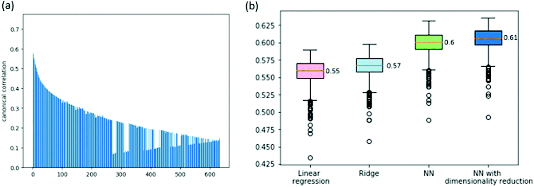 | ||
| Fig. 1 (a) CCA results for correlating a gene's expression profile and dependency vector. (b) Boxplot presenting the cross-validation Pearson correlations of the predictions of the cell lines’ genes dependencies, across various models. The orange line is the mean value across the cell lines and is equal to the ACC score of the model. | ||
In order to be able to predict gene dependencies across cell lines, we need to solve a multivariate regression task, in which every cell line is a regression's dependent variable. We note that while a previous work approached this problem, it was focused on a very small number of specific cell lines and used an obsolete version of the dependency data,8 hence we could not readily compare to it.
We attempt to predict the dependency data using various models. First, we tested a simple linear regression model. We got a cross-validation score of 0.55 ACC (average correlation coefficient across cell lines and folds, see Methods; Spearman correlation of 0.37). This confirms that a gene expression profile is a very good predictor of the gene's dependencies. Next, we attempted to improve this result by adding L2 regularization to the linear model (ridge regression). This yielded a slight improvement to an ACC of 0.57 (Spearman correlation of 0.38). Last, we attempted to use a non-linear model to improve performance further. To this end, we built a feed-forward neural network model with a non-linear activation function. Our cross-validation test tunes the hyperparameters that concern the network architecture (i.e., number of hidden layers and number of neurons per layer, see Methods). This yielded a further improvement to an ACC of 0.6 (Spearman correlation of 0.385).
In order to further improve performance, we explored the impact of dimensionality reduction of the gene expression data using the CCA results. We observed that the correlations of the different CCA components are high (Fig. 1a) and so we fed the CCA-reduced expression data as features to the neural network model, with the data dimension as a hyperparameter. Altogether, this improved scheme led to an ACC score of 0.61 (Spearman correlation of 0.39). The full results are summarized in Fig. 1b.
The second prediction problem we consider is the prediction of gene dependencies in yet unobserved cell lines (or samples). First, we study the gene dependency data distribution. A plot of gene dependencies is given in Fig. 2. From the plot, it is evident that genes can be roughly classified to ∼13![[thin space (1/6-em)]](https://www.rsc.org/images/entities/char_2009.gif) 000 “constant”, i.e., close to 0 or close to 1 with low standard deviation (<0.1), and ∼5000 “variable”, i.e., between 0 and 1 with high standard deviation (>0.1).
000 “constant”, i.e., close to 0 or close to 1 with low standard deviation (<0.1), and ∼5000 “variable”, i.e., between 0 and 1 with high standard deviation (>0.1).
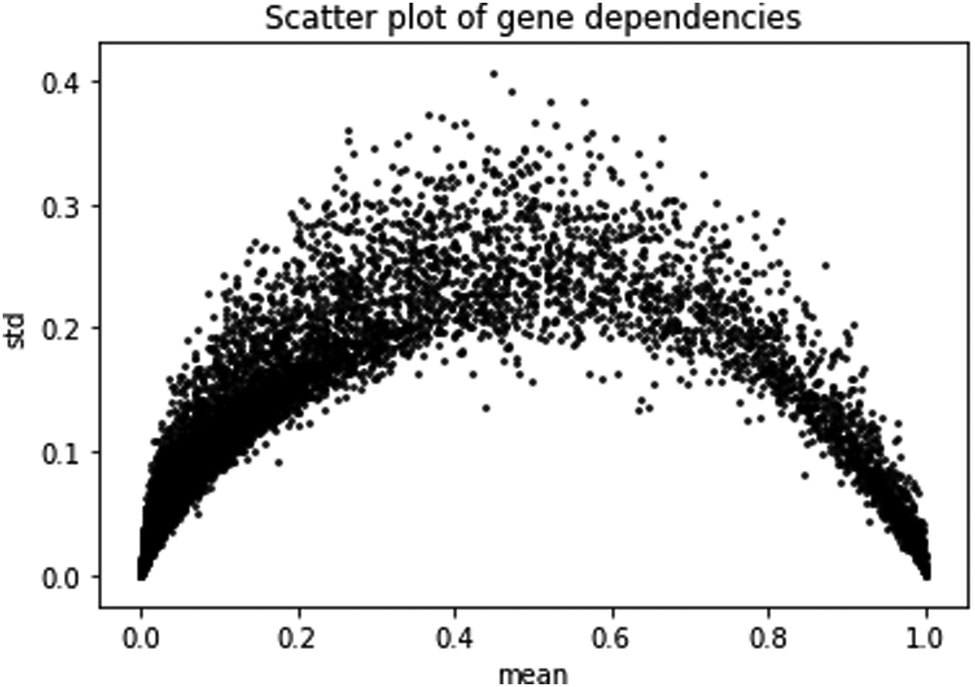 | ||
| Fig. 2 Scatter plot of gene dependencies. Shown are the mean and standard deviation of the dependencies of each gene across cell lines. | ||
We focus here on the prediction of dependencies for the variable group of genes. Such a prediction problem is challenging since a direct prediction of the dependency values (e.g., using linear regression) requires learning about 90 M parameters while the number of data points is around 30 M. Similarly, for simple neural network architecture, the relatively small number of data points for training greatly limits the number and size of the hidden layers (see Methods). Indeed, a neural network model without dimensionality reduction provided poor results. Specifically, it performed best with 3 hidden layers of 100 neurons each, yielding an ACC across all genes of 0.14, with 1172 genes having a correlation higher than 0.2.
To tackle the dimensionality challenge we aimed to reduce the data dimension. However, the dimensions of both the expression data and the dependency data, are much larger than the sample size (the number of cell lines). In such a setting, the canonical correlations can be extremely misleading as they are generally substantially overestimated.16 Indeed, when we applied CCA to these data, the resulting canonical correlations were always one, implying that they do not carry any information about the true population canonical correlations.
Therefore, we chose to reduce the dimension of the independent variables of expression data and the dependent variable of dependency values using autoencoders.17 An autoencoder consists of an encoder and a decoder. Given the input data n-dimensional data point x, the encoder first maps x to its latent d-dimensional representation z = E(x), where typically d < n. The decoder then maps z to a reconstruction x′ = D(z) (also n-dimensional), with reconstruction error measuring the deviation between x and x′. The encoder consists of an input layer, one hidden layer, and an encoded layer. The decoder starts at the encoded layer, uses one hidden layer and finally outputs the reconstruction layer (see Fig. 3). The parameters of the network are updated via backpropagation with the goal of minimizing the reconstruction error (see Methods). By restricting the latent space to lower dimensionality than the input space (d < n) the trained autoencoder parametrizes a low-dimensional nonlinear manifold that captures the data structure.
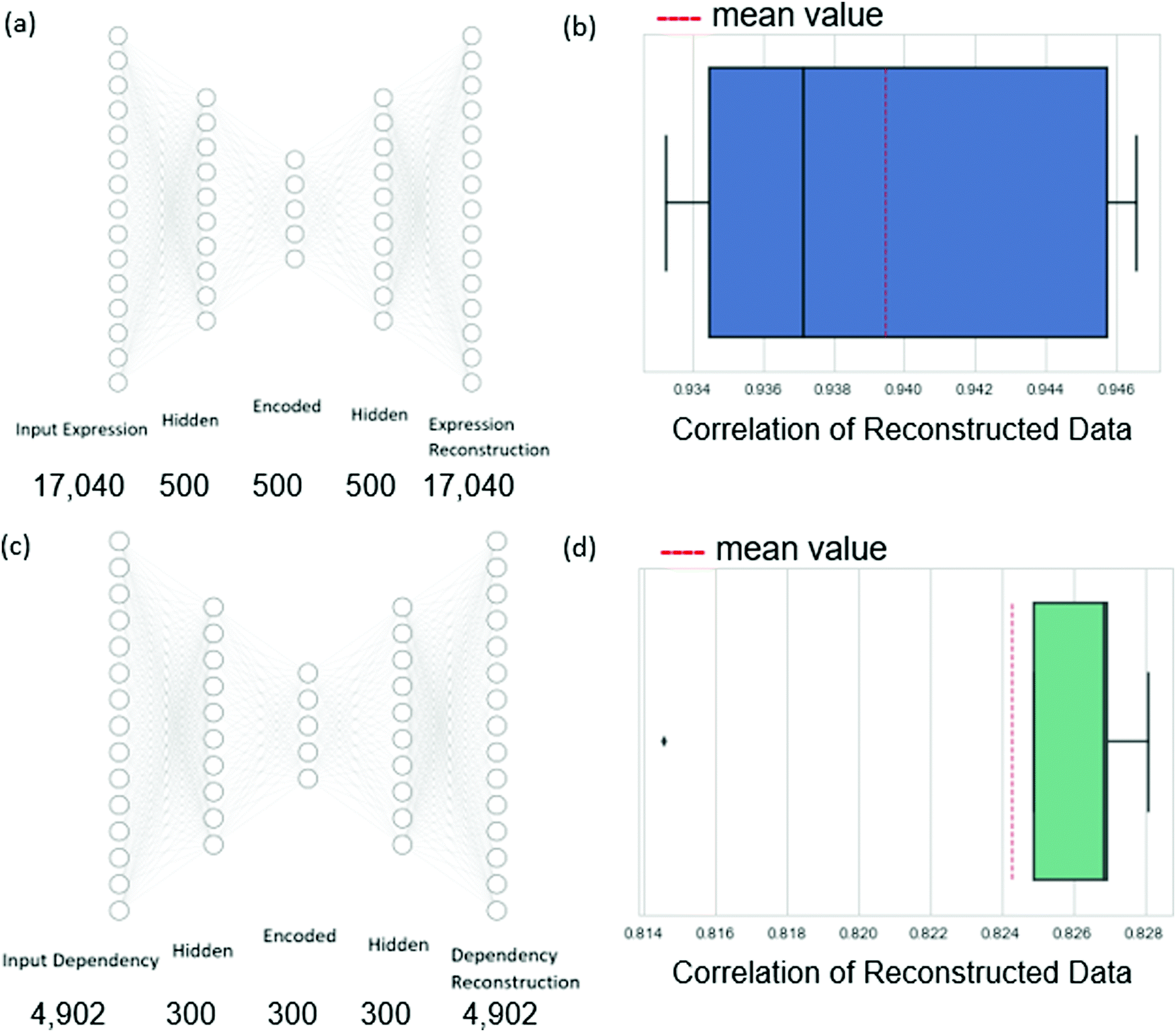 | ||
| Fig. 3 Illustration of the autoencoder model architecture and results. (a and c) The network architecture of the expression and dependency autoencoders respectively, along with the number of neurons at each layer. (b and d) Boxplots of the cross-validation reconstruction result for expression and dependency data respectively. The scores displayed are the Pearson correlation averages between the original data and the reconstructed data. | ||
In more detail, the dependency data spans 630 cell lines, each with expression measurements of 18239 genes and 4902 measurements of dependency values for variable genes. We filtered out from the input genes for which the expression data has more than 80% zero values to ensure sufficient information through the cross-validation iterations. This resulted in a final set of 17040 genes. Autoencoders were applied to reduce the dimension of the expression profiles to 500 and the dependency profiles to 300 (these values were chosen to respect the volume of the data available for training, see Methods). We evaluated the autoencoders in a 5-fold cross-validation setting. We found that the average Pearson correlation between the expression data and the reconstructed expression data was 0.94, while the same measure of the dependency data autoencoder was 0.82. These high correlations indicate that the dimension-reduced profiles can well represent the original data.
When combining the autoencoders into the neural network regression scheme, we could explore larger layers (Methods), achieving the best results with 6 hidden layers of 600 neurons each. The average Pearson correlation across all genes was 0.18, while 1639 genes had a correlation higher than 0.2. These results and the comparison to a neural network that does not use the autoencoders are summarized in Fig. 4.
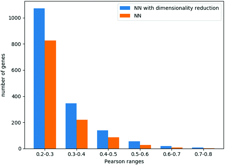 | ||
| Fig. 4 Model performance in predicting gene dependencies. For all tested models, shown is a histogram of gene number as a function of the correlation between their predicted and real values. The majority of the genes (15401) had a correlation below 0.2 and are not presented in this figure. | ||
A model for predicting drug sensitivity data
As drug treatment often leads to the inhibition of the drug's targets,18 we reasoned that our success in predicting gene dependencies across cell lines could imply that we could perform a similar prediction for drug sensitivities. In contrast to dependency data, drug sensitivities have relatively high standard deviations across different cell lines, hence there was no need to filter low-variance drugs. Altogether, we analyzed data from 3464 drugs with known targets across 524 cell lines.We explored two sources of information for the prediction task. First, as above, we used gene expression data. Specifically, for every drug, we obtained its set of known targets (from DepMap) and formed mean expression vectors for those targets across the 524 cell lines. For this task, we first explored ridge regression as a linear model that achieves a cross-validation score of 0.36 ACC. Second, we use a neural network regression model which presents a cross-validation score of 0.39 ACC.
Next, we wish to explore the prediction of the drug sensitivities based on the corresponding gene dependencies. We formed mean vectors from the dependency data of the drug's targets, similar to the mean gene expression as before. Applying ridge regression to these data yielded an ACC score of 0.37. A neural network regression model performed better with a cross-validation score of 0.39 ACC.
Finally, the combination of the two data sources used above can be exploited for predicting drug sensitivities. To this end, we concatenated the expression and dependency data and tested both a linear model and a neural network model. The linear model performance improved to an ACC of 0.39. The neural network model also benefits from utilizing both data sources, achieving an ACC score of 0.4. The results are summarized in Fig. 5.
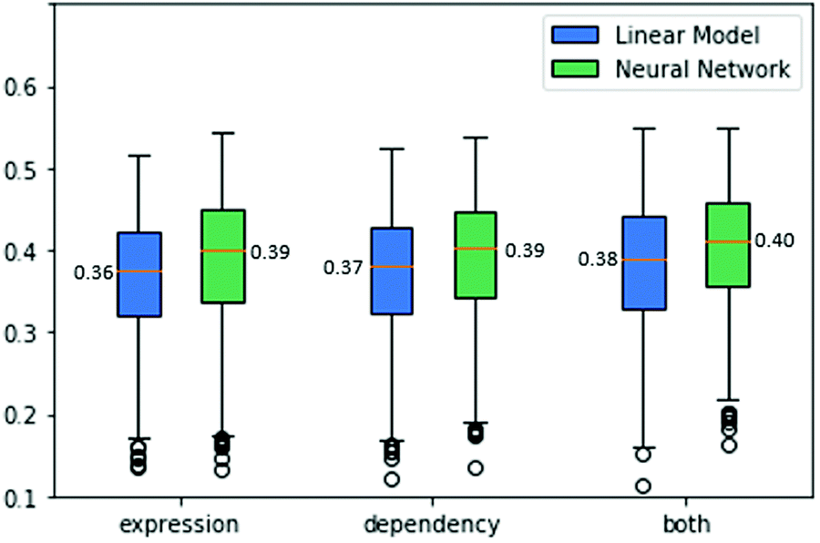 | ||
| Fig. 5 Drug sensitivity predictions. Each boxplot presents the cross-validation Pearson correlations of the predictions of the cell lines’ drug sensitivities. The predictions are obtained with linear models as well as neural networks, using gene expression information, gene dependency information and both. | ||
Conclusions
In this work, we tackled various prediction problems that concern the identification of cancer cell line vulnerabilities. We have shown the utility of deep learning models for predicting gene dependencies and drug sensitivities across genes and cell lines. To cope with the high number of predictive features, we combined dimensionality reduction strategies into our prediction framework, leading to improved predictions that outperform simpler models.Our work focused on predicting genetic dependencies from transcriptomics data as this remains the most abundant data type to date. Yet, our framework can be strengthened by combining other data types such as DNA methylation data, proteomics, interactome data, etc. In addition, while our algorithms achieved promising results, their performance in a real clinical setting where samples come from real patients will need to be assessed when such dependency data becomes available.
Methods
Achilles gene dependency data
The Achilles dataset19 contains the results of genome-scale CRISPR knockout screens for 18333 genes in 689 cell lines from the cancer cell line encyclopedia (CCLE) project.20 The Achilles gene dependency dataset contains for each of the tested genes and cell lines the probability that knocking out the gene has a depletion effect. The data were corrected using the CERES algorithm.7 As can be observed in Fig. 1, most genes are either near 0 (no effect) or near 1 (significant effect across all cell lines) with the rest of the genes having a high standard deviation (>0.1). We call the latter genes variable.
Overall, 4902 genes were variable, 12500 near 0 (precisely, mean <0.5 and std <0.1) and 837 near 1 (precisely, mean >0.5 and std <0.1). When learning the variable gene dependencies, we learned from the 630 cell lines for which the dependency data for all these genes were given.
CCLE expression data
CCLE expression data contains RNAseq TPM (transcript per kilobase million) measurements, which were obtained with the RSEM software package.21 The total number of genes in the dataset is 19144. However, we used only genes that also appear in the dependency dataset. The total number of genes that appear in both datasets is 18239.
Drug sensitivity data
The drug sensitivity dataset22 contains the results of pooled-cell line chemical-perturbation viability screens for 4518 compounds screened against 578 cell lines. The dataset can be downloaded from the DepMap website (http://primary_replicate_collapsed_logfold_change_v2.csv). We filtered out cell lines with more than 75% missing data, leaving us with 524 cell lines. Missing entries were completed by the mean sensitivity value of the corresponding drug. We focused on 3464 drugs with known targets, as taken from primary-screen-replicate-treatment-info published on the DepMap website.Cross-validation and hyperparameter tuning
In our regression models, we aim to present results that are unbiased by train-test splitting, and by hyperparameter tuning. The score we present for each model is an average score of a 5-fold cross-validation test. For each fold, the current fold is marked as test data while the rest is used for train-validation. For each train-validation, we randomly split it into a train (80%) and validation (20%). We run the model with different sets of hyperparameters, and validate it on the validation data. We choose the hyperparameter configuration that performed the best and we use it for training on the entire train-validation data. Finally, we evaluate the model on the test data. This process is repeated for every fold, and the score is the average score over all folds.Evaluation of a regression task is typically made by the Pearson correlation coefficient. It is preferable on measures like mean squared error, since the value of the error can be of any range. As the regression problems we solve have multiple dependent variables, we compute the correlation for every variable separately and then average the results across all of them,23 we call it ACC (average correlation coefficient). The score of a cross-validation test is thus the average ACC across all test folds.
Canonical correlation analysis
Canonical correlation analysis (CCA) is a multivariate analysis between two data views. The CCA objective is to project the two data views onto a shared space such that the correlation between the projections is maximal. The first component is the absolute optimal solution, the i-th component is the maximal solution such that it is orthogonal to the previous components (see eqn (1)). This process is repeated until no more pairs are found. The implementation of the CCA we used in this paper was given by the Scikit-Learn library.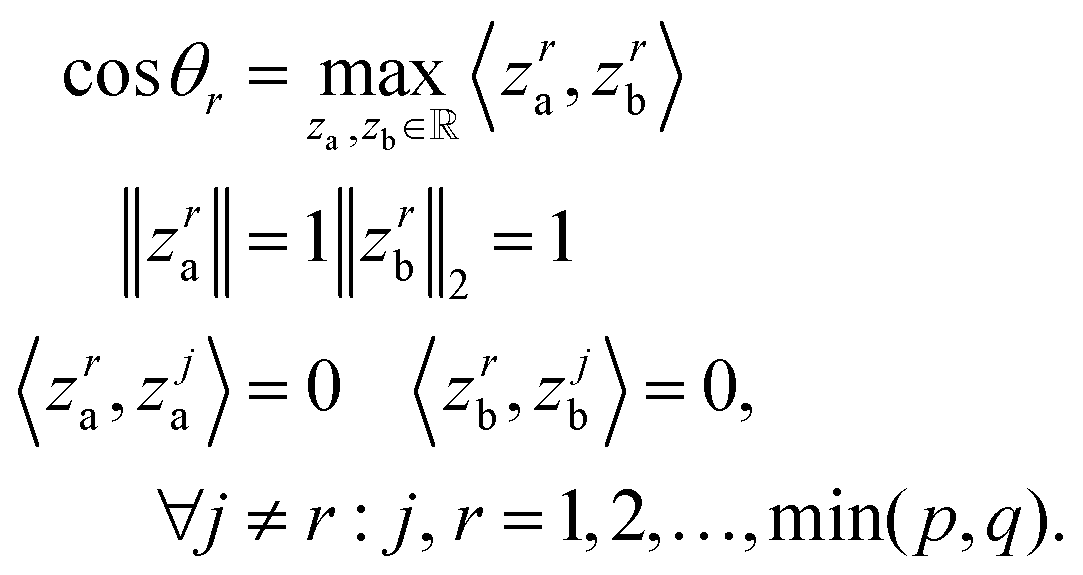 | (1) |
Neural network construction
Our models were based on a feedforward multilayer neural network, which enables us to create increasingly more complex nonlinear functions as its number of hidden layers increases. The network generally consists of at least three layers, one input layer, one output layer, and one or more hidden layers. Every layer of the neural network consists of a linear function and a nonlinear activation function. Note that without the activation functions, any neural network reduces to a linear regression model, as any composition of linear functions is also linear. The error computed from the output layer is back-propagated through the network, and the weights are modified according to their contribution to the error function. For our models, we chose a hyperbolic tangent as it is a common activation function for any layer in regression tasks and for hidden layers in classification tasks. For the optimization task, we chose mean squared error loss and the Adam optimizer with a learning rate of 10−4.In order to choose the number and size of layers in the deep network, we used cross-validation. We explored 1–10 hidden layers and layer sizes of 100 to 1000. We limited the search to architectures in which the number of weights to learn is at most the number of available data points to train on. In addition, we limited the search so that the number of neurons of a hidden layer is roughly between the sizes of the input and output layers.
Autoencoder construction
For encoding the gene expression data and the dependency data, we trained two autoencoders. For the autoencoders of the expression data, the input and output layers had the size of the gene expression vector that describes a cell line (17040). For the autoencoder of the dependency data, the input and output layers had the same number of neurons as the number of genes for which we wish to predict their dependencies (4902). The architecture tuning and parameter learning were performed similarly to the regression networks.
Conflicts of interest
There are no conflicts to declare.References
- D. M. Munoz, et al., CRISPR Screens Provide a Comprehensive Assessment of Cancer Vulnerabilities but Generate False-Positive Hits for Highly Amplified Genomic Regions, Cancer Discovery, 2016, 6(8), 900–913 CrossRef CAS.
- B. Luo, et al., Highly parallel identification of essential genes in cancer cells, Proc. Natl. Acad. Sci. U. S. A., 2008, 105(51), 20380–20385 CrossRef CAS.
- R. Marcotte, et al., Essential gene profiles in breast, pancreatic, and ovarian cancer cells, Cancer Discovery, 2012, 2(2), 172–189 CrossRef CAS.
- J. G. Doench, Am I ready for CRISPR? A user's guide to genetic screens, Nat. Rev. Genet., 2018, 19(2), 67–80 CrossRef CAS.
- J. G. Doench, et al., Optimized sgRNA design to maximize activity and minimize off-target effects of CRISPR-Cas9, Nat. Biotechnol., 2016, 34(2), 184–191 CrossRef CAS.
- A. de Weck, et al., Correction of copy number induced false positives in CRISPR screens, PLoS Comput. Biol., 2018, 14(7), e1006279 CrossRef.
- R. M. Meyers, et al., Computational correction of copy number effect improves specificity of CRISPR-Cas9 essentiality screens in cancer cells, Nat. Genet., 2017, 49(12), 1779–1784 CrossRef CAS.
- G. Benstead-Hume, S. K. Wooller, S. Dias and L. Woodbine, Biological network topology features predict gene dependencies in cancer cell lines, bioRxiv, 2019 DOI:10.1101/751776.
- J. Barretina, et al., Addendum: The Cancer Cell Line Encyclopedia enables predictive modelling of anticancer drug sensitivity, Nature, 2019, 565(7738), E5–E6 CrossRef CAS.
- Z. Dong, et al., Anticancer drug sensitivity prediction in cell lines from baseline gene expression through recursive feature selection, BMC Cancer, 2015, 15, 489 CrossRef.
- G. Riddick, et al., Predicting in vitro drug sensitivity using Random Forests, Bioinformatics, 2011, 27(2), 220–224 CrossRef CAS.
- L. Nguyen, C. C. Dang and P. J. Ballester, Systematic assessment of multi-gene predictors of pan-cancer cell line sensitivity to drugs exploiting gene expression data, F1000Research, 2016, 5, 2927 Search PubMed.
- L. Parca, et al., Modeling cancer drug response through drug-specific informative genes, Sci. Rep., 2019, 9(1), 15222 CrossRef.
- S. Naulaerts, M. P. Menden and P. J. Ballester, Concise Polygenic Models for Cancer-Specific Identification of Drug-Sensitive Tumors from Their Multi-Omics Profiles, Biomolecules, 2020, 10(6), 963 CrossRef CAS.
- N.-N. Guan, Y. Zhao, C.-C. Wang, J.-Q. Li, X. Chen and X. Piao, Anticancer Drug Response Prediction in Cell Lines Using Weighted Graph Regularized Matrix Factorization, Mol. Ther.–Nucleic Acids, 2019, 17, 164–174 CrossRef CAS.
- Y. Song, P. J. Schreier, D. Ramírez and T. Hasija, Canonical correlation analysis of high-dimensional data with very small sample support, Signal Process., 2016, 128, 449–458 CrossRef.
- G. E. Hinton and R. R. Salakhutdinov, Reducing the dimensionality of data with neural networks, Science, 2006, 313(5786), 504–507 CrossRef CAS.
- R. Sawada, M. Iwata, Y. Tabei, H. Yamato and Y. Yamanishi, Predicting inhibitory and activatory drug targets by chemically and genetically perturbed transcriptome signatures, Sci. Rep., 2018, 8(1), 156 CrossRef.
- J. M. Dempster, et al., Extracting Biological Insights from the Project Achilles Genome-Scale CRISPR Screens in Cancer Cell Lines, bioRxiv, 2019 DOI:10.1101/720243.
- M. Ghandi, et al., Next-generation characterization of the Cancer Cell Line Encyclopedia, Nature, 2019, 569(7757), 503–508 CrossRef CAS.
- B. Li and C. N. Dewey, RSEM: accurate transcript quantification from RNA-Seq data with or without a reference genome, BMC Bioinf., 2011, 12, 323 CrossRef CAS.
- S. M. Corsello, et al., Non-oncology drugs are a source of previously unappreciated anti-cancer activity, Nat. Cancer, 2020, 1, 235–248 CrossRef.
- H. Borchani, G. Varando, C. Bielza and P. Larrañaga, A survey on multi-output regression, Wiley Interdiscip. Rev.: Data Min. Knowl. Discovery, 2015, 5(5), 216–233 Search PubMed.
| This journal is © The Royal Society of Chemistry 2021 |