
 Open Access Article
 This Open Access Article is licensed under a Creative Commons Attribution-Non Commercial 3.0 Unported Licence
Coarse-grained molecular dynamics study of the self-assembly of polyphilic bolaamphiphiles using the SAFT-γ Mie force field†
Maziar
Fayaz-Torshizi
and
Erich A.
Müller
 *
*
Department of Chemical Engineering, Imperial College London, London, UK. E-mail: e.muller@imperial.ac.uk
First published on 29th April 2021
Abstract
A methodology is outlined to parametrize coarse grained molecular models for the molecular dynamics simulation of liquid crystalline bolaamphiphiles (BAs). We employ a top down approach based on the use of the Statistical Associating Fluid Theory (SAFT) that provides a robust and transferable set of building blocks from the fitting of thermophysical properties of smaller molecules. The model is employed to characterise symmetric and asymmetric swallow-tailed BAs and to compare them with an isomeric T-shaped BA. Branching of the side chain of the BAs, leading to the swallow-tailed geometry generates a richness in the number and morphology of liquid crystal mesophases. The simulations elucidate some of the intriguing results observed in experiments.
Design, System, ApplicationThe paper focuses on the development of a molecular-based methodology to coarse-grain accurate force fields for use in simulations of soft matter. The force field parameters of small chemical moieties are optimized from fitting to experimental thermophysical properties of corresponding fluids (or families) using an appropriate analytical molecular equation of state (in this case the Statistical Associating Theory of Fluids, SAFT-γ). The resulting building blocks are then combined in a group-contribution approach to produce a force field for a larger, complex molecule. This optimization strategy produces very robust top-down effective potentials which can describe quantitatively the phase behaviour of complex and/or polyphilic molecular systems. The coarse-grained nature of the force fields allows order-of-magnitude increases in speed and system size over the corresponding fully atomistic descriptions. We showcase the procedure by applying it to a family of recently synthesized liquid crystals which tessellate 2-D space. These laterally-substituted bolaamphiphiles have very intriguing mesophases, which are captured in detail by the coarse-graining molecular dynamics simulations described in the manuscript. The general procedure described is, however, general in nature and can be translated directly to the study and design of other types of complex molecular systems. |
1 Introduction
The synthesis of materials that can self-assemble into ordered structures has become a ubiquitous topic in the field of physical sciences and engineering.1–4 The mesostructure of a material can significantly affect its physical properties,5 and this makes self-assemblying materials attractive in many applications such as catalysis,6,7 heat insulation,8 display devices,9 semiconductors, electronic, optical and photovoltaic devices.Bolaamphiphiles (BAs)10 are a group of molecules composed of two hydrophilic end groups, and a connecting hydrophobic group forming the molecular backbone. Rigid BAs behave like liquid crystals with smectic A (SmA), nematic and isotropic coexisting phases observed,11 commensurate with previous studies of both attractive12,13 and hard14,15 calamitic liquid crystals (Fig. 1 (Top)). Simulation studies11 have demonstrated that stronger self-attraction of the end groups of rigid bolaamphiphiles can reduce the size of the isotropic–nematic phase transition curve, and lead to formation of isotropic–SmA phase transition at lower temperatures. For molecules similar to the one presented in Fig. 1(Middle), the hydrogen bonding strength of the end groups is dominant and only isotropic–SmA phase transitions are observed experimentally.16
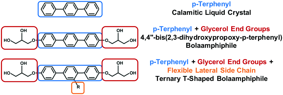 | ||
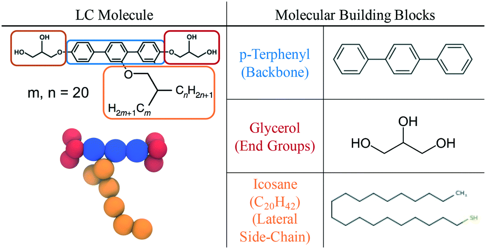
| Fig. 1 Top: The chemical structure of p-terphenyl, a calamitic. Middle: Bolaamphiphile 4,4′′-bis(2,3-dihydroxypropoxy-p-terphenyl). Bottom: T-shaped bolaamphiphile (BA) with a lateral side chain. | ||
Adding flexible side chain(s) to bolaamphiphilic liquid crystals, (Fig. 1, Bottom and 2), promotes the self-assembly of new mesophases.17 The lateral side chains disrupt the underlying smectic phase, leading to columnar phases with complex two-dimensional tiling patterns for shorter chains, and lamellar or three-dimensional network phases for the longer chains. The synthesis of rigid BAs with lateral side chains including alkyl,17,18 semiperfluoronated alkyl chains,19–25 polyether (facial amphiphiles),26 or carbosilane27 side chains have been reported and characterised.
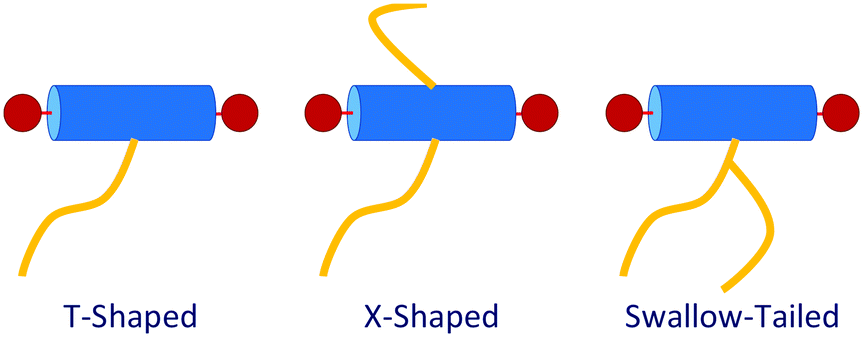 | ||
| Fig. 2 Structural variety of polyphilic BAs. | ||
T-shaped BAs with a single lateral side-chain have been the most extensively studied experimentally with 15 unique structures discovered to date.4,29,28 The sequence of some of the most common liquid crystalline phases seen in T-shaped BAs, upon increasing the size of the lateral chain, are depicted in Fig. 3. Typical BAs will exhibit a smectic ordering. The addition of very small side chains induce triangular columnar phases with a hexagonal p6mm symmetry. Increasing the size of the side chain leads to formation of square (p4mm), pentagonal (p2gg) and hexagonal (p6mm) columnar phases. Upon further increasing the length of lateral side chains, lamellar, hexagonally organised nano-wires and bicontinuous cubic networks have also been observed.28 X-shaped bolaamphiphiles (Fig. 2) with either the same moieties for the lateral chains or different groups can lead to combinations of these tiling patterns tessellating the 2-D plane perpendicular to the direction of the columns. In a particular example reported, one of the side chains is a short polyether chain which favours a triangular columnar phase, and the other a longer alkyl chain which induces square columnar phases (p4g phase).26 A particular system of X-shaped BA combining a semiperfluorinated chain and a carbosilane chain was shown to be able to produce up to three different polygons tessellating the plane: a square, a triangle and a rhombus,30 demonstrating the complexity of the self-assembling structures observed with BAs.
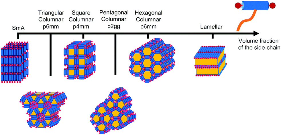 | ||
| Fig. 3 Example of a sequence of liquid crystalline phases formed by self-assembly of T-shaped BAs as observed upon increasing the volume fraction of the side-chain, adapted from ref. 28. | ||
Given the laborious and exhaustive process of synthesis and characterisation,31 the development of a complementary theoretical methodology to predict the structures for a given system a priori can become a cost effective and efficient approach in designing BAs. Detailed atomistic simulation of BA's is impractical as the length and time scales required to observe self-assembly are orders of magnitude larger than those accessible with current hardware. Notwithstanding, if one is willing to sacrifice some of the atomistic detail, the use of coarse-grained (CG) force fields allows the direct observation of self-assembly within a classical molecular dynamics simulation.32
In most CG methods, a reduction in the detail of the molecular description is sacrificed in favour of gains in terms of the complexity of the computational methods used in their modelling. The field of coarse-graining is still in development, and there are several general approaches to produce force fields at this level of granularity. On one hand, there are approaches which start from an agreed fine-detailed model (e.g. an atomistically-detailed description) and integrate out degrees of freedom from this high-fidelity benchmark. In this category we encounter most of the proposals associated with iterative Boltzmann inversion (IBI) techniques.33,34 The IBI method relies on self-consistently adjusting a given potential to achieve a maximum likelihood fit with target structural data; typically the radial distribution function. This bottom-up approach is capable of producing accurate potentials, but typically suffers from a lack of transferability, i.e. the potentials become state-dependent and can only be trusted to reproduce the conditions for which they are parametrized.35,36 Other strategies of this kind are the force-matching techniques37 and the relative entropy procedures.38 On the other end of the spectrum, there are approaches where the force-fields are generated by attempting to reproduce in the most average way possible the macroscopic observable properties of molecules, typically invoking some level of group contribution model. Of significant mention are the Martini force field39,40 and the SAFT model41 which characterizes CG beads according to a fit of the free energy. These top-down methods excel at producing robust intermolecular potentials at the expense of the need to process a larger amount of information. It is, in this latter category, where the models described in this contribution fit in.
Following this approach, the first studies on the self-assembly of T-shaped BAs via molecular dynamics simulations were the works of Crane et al. investigating the phase behaviour of pure component42 and mixtures43 of BAs. The model proposed was based on Lennard-Jones (LJ) type potentials, which were not tuned nor fitted specifically to experimental data and were assigned plausible “order of magnitude” self and cross interactions. For weak interactions, the LJ potential was cut-off and shifted using a Weeks–Chandler–Anderson potential (WCA),44 which included all cross interactions and the self-interaction of the segments of the backbone, assuming weak π–π interaction of the phenyl groups. The end groups were modelled as attractive beads with a self-interaction of ε and the segments of the lateral side chain had a weaker self interaction of 0.5ε. All building blocks had the same size σ, with no efforts in relating the sizes of the segments to real molecules. For short side-chains with contour lengths of <5σ, triangular, square and hexagonal columnar phases were observed. Despite its simplitcity, the Crane model was exceedingly successful at reproducing experimental observations. For intermediate chain lengths, an asymmetric combination of pentagonal and hexagonal columns were present, which was attributed to the fact that pentagons cannot tessellate planes. For chains with contour lengths of 12σ, lamellar phases were observed.
The work of Crane et al.42 was complemented by the studies of Bates and Walker,46–48 who developed dissipative particle dynamics (DPD) models to study T-shaped and X-shaped BAs. The phases discovered by Bates and Walker for T-shaped bolaamphiphiles were commensurate with those observed by Crane et al. DPD has similar limitations to the Crane model: all segments in the model were of the same size, and here the backbone and the end groups were softer than the lateral side chain in terms of self-interaction. With a symmetric bolaamphiphilic molecule, only triangular columnar, square columnar, hexagonal columnar and lamellar phases were observed for T-shaped BAs.47 For X-shaped BAs, Archimedean tiling patterns combining triangles with hexagons and triangles with squares were observed. Neither the Crane or the Bates and Walker models were able to predict regular pentagonal columnar phases seen experimentally.26 However, by modifying the bolaamphiphile backbone and making it chemically asymmetric (with more hydrogen bonded segments on one side), it was possible to observe pentagonal columnar phases.49 This underscored the discrepancy between experimental observations and DPD simulations with the model developed by Bates and Walker, as none of the BA liquid crystals studied by experiments have been asymmetric. Liu et al.50 carried out further DPD studies of T-shaped BAs with a variable size of the hydrogen bonding end-groups. Again, triangular (p6mm), square (p4mm), hexagonal (p6mm), lamellar phases were observed. As in the work of Crane et al., highly irregular pentagonal columns were found, with the irregularity attributed to the incompatibility of the mesophase periodicity with the size of the box. It could be concluded that with particle based simulations, obtaining regular pentagonal columnar phases has been challenging. Recently, the pentagonal columnar (p2gg) phases have been modelled using self-consistent field theory (SCFT).51
These coarse-grained particle-based studies using “toy-models” provide qualitative insight into the mesophase behaviour of these materials. In this strategy different functional groups are made to be incompatible with each other, but the mapping to physical systems remains an issue as some approximations seem very restrictive (e.g. that the size of the segments in a molecular are all equal, that the interactions are very broadly described, etc.). The extent to which the assumptions in the models affect the phase behaviour observed in the simulations is not known. For example, regular pentagonal columnar phases have only been observed in systems that are not chemically representable.
Recently, a third class of BAs (labelled swallow-tailed) has been synthesised. Swallow-tailed BAs, as presented in Fig. 2, are a class of liquid crystals that have a branched lateral side-chain. The effect of branching is highly significant. While for T shaped and X shaped BAs the phase behaviour can be understood in terms of the volume fraction of the lateral side chains (Fig. 3) such an analysis is clearly inadequate for swallow-tailed BAs. Fig. 4, adapted from the work of Poppe et al.45 describes how the morphology of the branching has an effect on self-assembled structures. All three molecules presented in Fig. 4 have the same molecular weight. Poppe et al. discovered some of the most complex tiling patterns with BAs, with pentagonal–hexagonal and pentagonal–octagonal tiles tessellating the plane. This was achieved by transforming a BA with a single side chain of 20 carbons into one with 2 alkyl branches of different length but with the same total number of carbons (20).
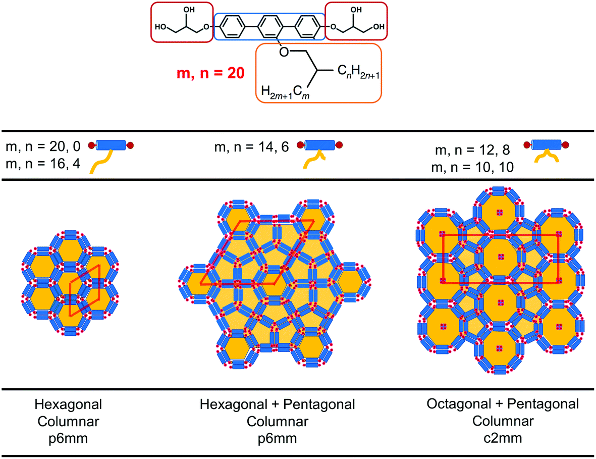 | ||
| Fig. 4 Experimentally observed mesophases for the swallow-tailed BAs studied in this work. Different mesophases are observed not by changing the volume fraction of the lateral side chain, but by changing the degree of branching, whilst conserving the volume fraction of all moieties. Adapted from Poppe et al.45 | ||
The main characteristic feature of swallow-tail BAs is that unlike all previous studies where the volume fraction of the side chains was the key factor in determining the mesophase structure, the volume fraction of the flexible chains is kept constant, and the geometry of the side chain becomes the key factor in self-assembly.
There has recently been one simulation study of swallow-tailed BAs, with a focus on very long lateral side-chains.52 Employing the Crane et al. model, no attempt was made to study any of the complex phases presented in Fig. 4 or to test the ability of the Crane model in predicting the two-dimensional tiling patterns of these zeolite-like liquid crystals. Moreover, like the previous studies, the effect of the volume fraction of the side-chain segments was the focus of that study, and not the effect of the degree of branching on mesophase behaviour. In that study, gyroid phases and plumbers nightmare phases were observed, which are novel for liquid crystalline materials.
This manuscript reports the development of a CG model of BAs that is structurally and thermodynamically consistent with experimental systems. The molecular parameters of each constituent building block are derived from the macroscopic thermodynamic properties of smaller, chemically related, molecules employing the SAFT-γ Mie approach,41 while the intramolecular potential is regressed from an atomistically detailed model. It is expected that the enhanced representability of this model provides advantages in the design of BAs. Unlike the phenomenological studies undertaken previously, SAFT-γ Mie CG simulations are quantitatively predictive approaches where, for example, the transition temperatures and the size of the ordered structures can be directly related to the physical molecule studied.
2 Methodology
In this work, an alkyl substituted 4,4′′-bis(2,3-dihydroxypropoxy-p-terphenyl) molecule is coarse-grained (Fig. 1(Bottom)) following the strategies employed for other complex molecules such as surfactants,53 asphaltenes,54 polymers55–58 and liquid crystals.59We choose to construct a molecular model by stitching together “building blocks” of smaller well-defined molecules for which there exists experimental thermophysical data, which allows the top-down parametrisation of the force fields. In order to coarse-grain this molecule, first the three main functional groups are defined.
2.1 Defining the building blocks
Table 1 is a summary of the coarse-graining building blocks employed in this work. The swallow-tailed bolaamphiphile is segmented into three distinct functional groups: a rigid backbone which shares its parameters with a p-terphenyl molecule, two end groups that are modelled as glycerol molecules, and a swallow-tail moiety which shares parameters with icosane, (C20H42). Although there is a mismatch between the molecules used as surrogates and the corresponding segments of the BA, the CG model assumes that the physical interactions between groups of atoms do not change drastically within a given family, i.e. a –(CH2)3– group in the middle of an alkane will have the same properties regardless of the rest of the atoms in the molecule. While clearly an approximation, this group contribution model is the basis of most CG approaches. Some atoms seem to be missing in the representation the molecule, e.g. glycerol has an extra hydrogen atom as compared to an end group, or the side chains modeled as alkanes are missing the connecting ether. These omissions are unavoidable in our model and their effects are expected to be minor.
|
2.2 CG representation of the BA
Given the definitions of the constituent moieties, the next step is to define a CG representation of the molecule. As will be explained in section 2.3, the theory used to obtain the force field parameters, SAFT-γ Mie, assumes molecules are chains of tangentially bonded coarse-grained segments. The number of segments representing each of the groups is decided heuristically, attempting to minimise the number of segments to reduce computational expenses, whilst keeping the model as representable of the real system as possible.The rigid backbone of the BA molecule is a p-terphenyl group with three phenyl rings attached to each other linearly. In the CG representation, each phenyl ring is represented by a CG sphere. Icosane, a C20n-alkane, is modelled as a chain of 6 beads, in agreement with previous studies on alkanes.60 Glycerol end groups are modelled as 3 segment models each, assigning one hydrogen bonding sites to each CG segment. The schematic of the CG representation of the BA can be seen in Fig. 1.
To simulate swallow-tailed BAs, alkane segments need to be rearranged from the linear chain of the icosane to branched chains. Given that a 6 bead model is used to represent icosane, every 3.7 (≈4) united atom carbons maps into a segment. The number of CG segments in each chain of the swallow-tail for each of the molecules in Fig. 4 is given in Table 2.
| Molecule | m | n | m CG | n CG |
|---|---|---|---|---|
| 1 (T-shaped BA) | 20 | 0 | 6 | 0 |
| 2 | 14 | 6 | 5 | 1 |
| 3 | 10 | 10 | 3 | 3 |
2.3 SAFT-γ Mie interaction parameters
Fig. 5 summarizes the general parameter fitting procedure employed to determine the SAFT CG force field. An analytical equation of state (SAFT-γ Mie EoS61) is employed to correlate the fluid phase properties (vapour pressures and saturated liquid density) of smaller building blocks and determine the molecular parameters (ε, σ, λ) of each “monomer” segment. The alignment of the EoS with the underlying Hamiltonian allows the use of the fitted parameters directly in a force field without further adjustments. The non-bonded force field is of a Mie form: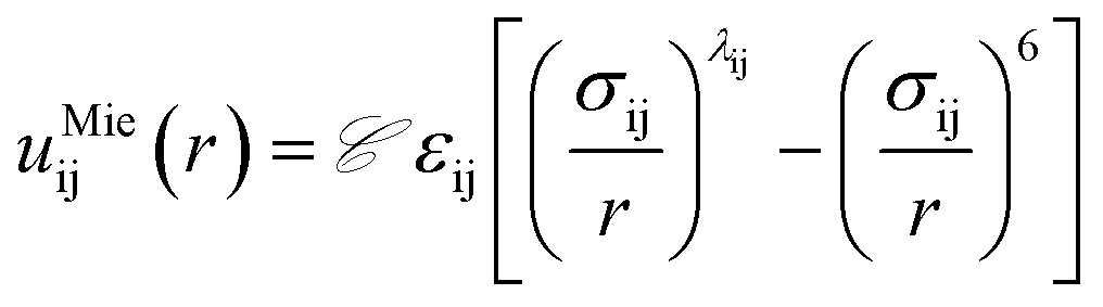 | (1) |
![[capital script C]](https://www.rsc.org/images/entities/i_char_e522.gif) is a pre-factor:
is a pre-factor: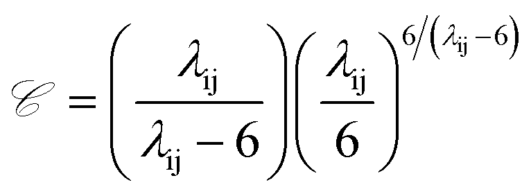 | (2) |
 | ||
| Fig. 5 Schematic of the coarse-graining methodology used in this work. | ||
Self-species force field parameters are obtained using correlations to thermophysical data, and cross species interactions are defined using combining rules, with the arithmetic mean and a geometric mean used to calculate values of σ and (λ − 3) respectively. The value of ε, is also calculated by including an extra binary interaction parameter, kij used to fine-tune the cross species interactions to experimental data:
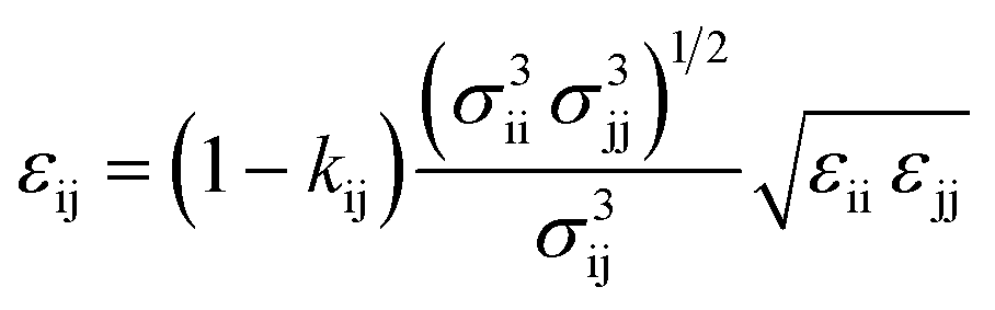 | (3) |
A particular challenge in fitting cross-interaction parameters is a lack of experimental data. To obtain cross interaction parameters, two pathways were taken:
1. Finding experimental data for mixtures of components most similar to the molecules presented in Table 1: e.g. instead of icosane using n-heptane, and instead of glycerol using ethanediol, where experimental solubility of p-terphenyl in those solvents are known, and transferring the kij parameters obtained there in for the moieties in the BA.
2. Using the current SAFT-γ EoS library62 of united atom groups to build the molecules in Table 1 and generating pseudo-experimental data. Using the pseudo-experimental data, cross interaction parameters are then fitted to these data. The current SAFT-γ library has many small united atom groups, but these models cannot be used in simulation due to the presence of parameters that currently cannot be modelled in simulation.
A detailed discussion, is included in the ESI,† where the form of the intermolecular potentials for self-species, cross species, as well as the parameter estimation procedures are discussed in detail.
Intramolecular bond stretching and bending of a harmonic nature are imported from atomistic simulations of the corresponding building blocks:
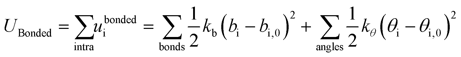 | (4) |
2.4 Simulation details
For each simulation, 2400 BA molecules (corresponding to ≈100![[thin space (1/6-em)]](https://www.rsc.org/images/entities/char_2009.gif) 000 atoms) are randomly placed in a simulation box which is compressed at 100 bar isotropically. After reaching a dense phase, NσT simulations were run with a Nosé–Hoover thermostat63,64 and Parrinello-Rahman barostat65 with a time-step of 0.01 ps, at different temperatures ranging from 450 to 300 K. During the equilibration, anisotropic pressure coupling is used. Each pressure tensor is fixed independently from other pressure tensors, allowing the simulation box to expand or compress in different directions with the angles of the box also being relaxed. Not only this helps in faster equilibration of the system, this type of expansion of the simulation box allows for the system to find the correct periodicity for the system, preventing molecules from being trapped in local minima and artificial structures.
000 atoms) are randomly placed in a simulation box which is compressed at 100 bar isotropically. After reaching a dense phase, NσT simulations were run with a Nosé–Hoover thermostat63,64 and Parrinello-Rahman barostat65 with a time-step of 0.01 ps, at different temperatures ranging from 450 to 300 K. During the equilibration, anisotropic pressure coupling is used. Each pressure tensor is fixed independently from other pressure tensors, allowing the simulation box to expand or compress in different directions with the angles of the box also being relaxed. Not only this helps in faster equilibration of the system, this type of expansion of the simulation box allows for the system to find the correct periodicity for the system, preventing molecules from being trapped in local minima and artificial structures.
The SAFT model, unlike previous studies, uses soft Mie interactions to simulate real systems. This means that equilibration times can take longer than the stiffer Crane models. Most of the simulations presented in this work required more than 500 million time-steps (5 μs). Given the current computing capacities, equilibration from random position of molecules takes about a week on a high specification 48 core processor. The cut-off employed in the system is set to 1.5 nm, approximately 3 σ of the largest segment. All simulations were carried out using GROMACS 5.1 (ref. 66) on Imperial College HPC clusters and on the Thomas cluster.
2.5 Phase characterisation and order parameters
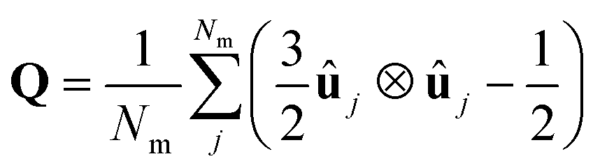 | (5) |
Once the director is calculated, it is possible to calculate the S2 nematic order parameters:
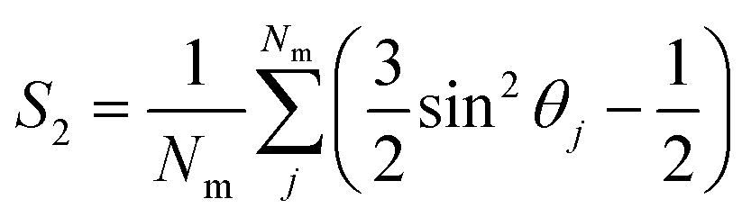 | (6) |
 | (7) |
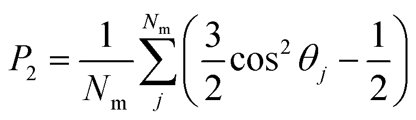
The director and the nematic order parameter allow one to calculate the degree of alignment of the molecules. To clearly characterise the specific structures of the LC phases seen in simulations, other metrics are required. For regular polygonal columnar phases, the planar orientational order parameter can be used:
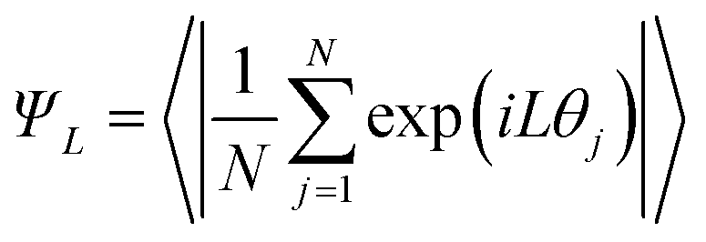 | (8) |
For superlattices, such as the pentagonal–hexagonal phase (presented in Fig. 4), and for 3-dimensional network phases, it is not possible to use the planar orientational order parameter. Therefore, for these phases, distribution functions and structure factors are more relevant.
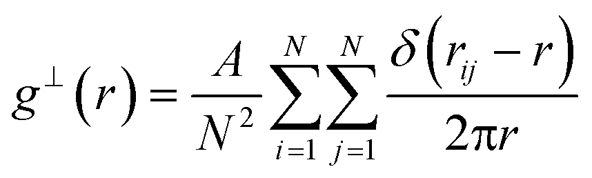
The planar 2-D radial distribution function is calculated using the following equation:
 | (9) |
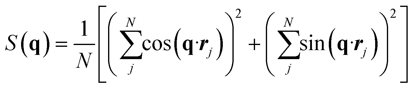
Following the work of Sun et al.,52 the structure factor is calculated using the following definition:
 | (10) |
 | (11) |
 | (12) |
3 Results
3.1 Parameter estimation
| Molecule | N CG | M W, CG | λ | ε/kB [K] | σ [Å] | AAD ρSatLiq % | AAD Pvap % |
|---|---|---|---|---|---|---|---|
| p-Terphenyl | 3 | 76.77 | 30.15 | 703.48 | 4.929 | 0.8 | 2.4 |
| Glycerol | 3 | 30.69 | 24.00 | 615.90 | 3.385 | 2.3 | 4.5 |
| Icosane | 6 | 47.09 | 24.70 | 453.10 | 4.487 | 4.6 | 9.6 |
The comparison between the calculations of the EoS using the fitted parameters and experimental data is presented in Fig. 6. Simulation data are also presented in Fig. 6, with calculations done after adding intramolecular interaction parameters.
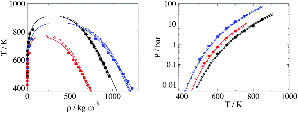 | ||
| Fig. 6 Comparison of theory (solid lines), experimental data (open symbols) and MD simulation (solid symbols) for the three different molecules used to model the BA. The black, blue and red colors correspond to p-terphenyl, glycerol and icosane respectively. Left Temperature vs. density and Right vapour pressure vs. temperature. | ||
The shape of the T-ρ phase envelope for icosane is slightly different in the EoS to that of the experimental data, which could be due to the different method of parametrisation using a corresponding states approach74 instead of directly fitting the parameters directly to experimental data. Moreover, for glycerol the theory overestimates the liquid densities at lower temperatures. This is an effect of hydrogen bonding in glycerol molecules (which is not considered explicitly in our models), where the structural changes at lower temperatures cause the fluid to have a lower density than expected. The overall error in density is low with an AAD of 2.3% for saturation liquid density. More details about thermodynamic properties of the self-interaction parameters can be found in the ESI.†
To calculate cross interactions, molecules are built by using SAFT-γ Mie UA (united atom) segments as building blocks. These united atom models have parameters related to the shape factor and association which cannot be used directly in molecular simulations, however are robust enough to calculate thermophysical properties of many molecules. For a review of the prediction capabilities of phase behaviour of complex molecules and the latest table of parameters one could refer to recent literature.62,75 The details of the fitting procedure are provided in the ESI.†
A summary of all the kij parameters used in this work is given in Table 4. Positive values of the kij indicate a significant repulsion between the different building blocks. Binary interaction parameters are symmetric, i.e. kij = kji.
| Mixture | k ij |
|---|---|
| p-Terphenyl–glycerol | 0.126 |
| p-Terphenyl–icosane | 0.112 |
| Glycerol–icosane | 0.145 |
Previous simulation studies of alkanes using SAFT-γ Mie have studied the intramolecular potentials of the alkanes, using a Boltzmann inversion method. Rahman et al.76 used TraPPE UA77 models to find optimal intramolecular interaction parameters for n-alkanes, with each CG segment representing 3 UA carbons. In this work, therefore, it was deemed unnecessary to fit the angle potentials of icosane, with the angle potentials fitted by Rahman et al. were used directly in this work. For alkanes, it was found that the optimal angle, θ, between three neighbouring CG groups, each representing three UA carbons, was 158° with kθ of 22 kJ mol−1 rad−2.
For the glycerol group, the angle potentials parameters were assumed to be the same as the angle between three backbone carbons of 1,3-propanediol as parametrised by TraPPE.78 Although this is a gross approximation, the angle potential of the glycerol groups is not expected to significantly affect mesophase behaviour as the size of each glycerol segment is much smaller than the size of each icosane or p-terphenyl segments, meaning chain stretching is not significant for glycerol. Therefore, an approximate set of parameters were used to qualitatively describe the intramolecular potentials of glycerol end groups.
For the rigid backbone, no literature studies of intramolecular potentials of CG models were found, and it was difficult to assume parameters for the angle potentials. Therefore, it was decided to find realistic angle potentials by fitting a potential to the probability distribution of the angles between the three phenyl rings in a p-terphenyl backbone using atomistic OPLS-AA simulations.79
In terms of bond stretching potential, the equilibrium bond distance between any two neighbouring segments is the same as σij of the non-bonded interactions and the bond constant kb for all species was set to 6130 kJ mol−1 nm, following previous work.76 Further discussions on the parameter estimation could be found in the ESI.† The results are summarised in Table 5.
| Beads | Angle/° | k θ /kJ mol−1 rad−2 | |
|---|---|---|---|
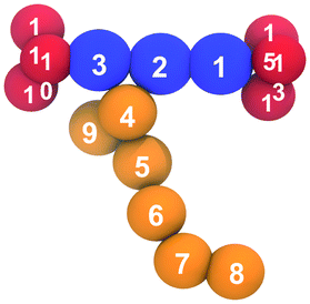
|
1–2–3 | 180 | 225 |
| 2–3–10 | 180 | 225 | |
| 2–1–13 | 180 | 225 | |
| 11–10–12 | 109 | 420 | |
| 14–13–15 | 109 | 420 | |
| 1–2–4 | 120 | 22 | |
| 4–5–6 | 158 | 22 | |
| 5–6–7 | 158 | 22 | |
| 6–7–8 | 158 | 22 |
3.2 Simulation of bolaamphiphiles
The three swallow-tail molecules studied in the work can be seen in Fig. 7. Details of LC phase behaviour of p-terphenyl and BAs without any lateral side chains can be found in the ESI.†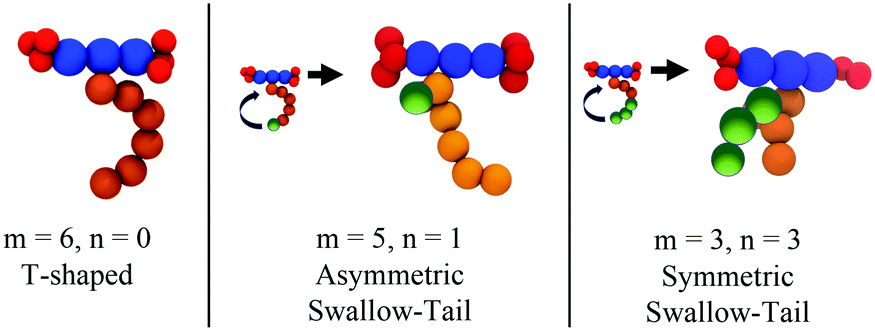 | ||
| Fig. 7 The structure of a T-shaped BA as it compares to the swallow-tailed BAs studied in this work. | ||
 | ||
| Fig. 8 Top Snapshots of an equilibrium configuration of self-assembled T-shaped BAs composed of side chain of C20H41 (m = 6, n = 0). The BAs self-assemble into a hexagonal columnar phase. Bottom snapshots of an equilibrium configuration of self-assembled asymmetric swallow-tail BAs composed, with one tail being C14H29 and the other C6H13 (m = 5, n = 1). T = 380 K, P = 1 bar. Colours are defined in Table 5. | ||
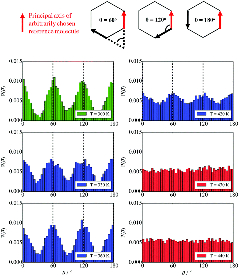 | ||
| Fig. 9 The distribution of angles between the principal axes of the backbone of an arbitrary BA and the rigid backbones of all other BAs in the simulation at different temperatures. Green represents a crystalline solid phase, red represents isotropic phase where no peaks are observed, and blue represents the liquid crystalline phase. | ||
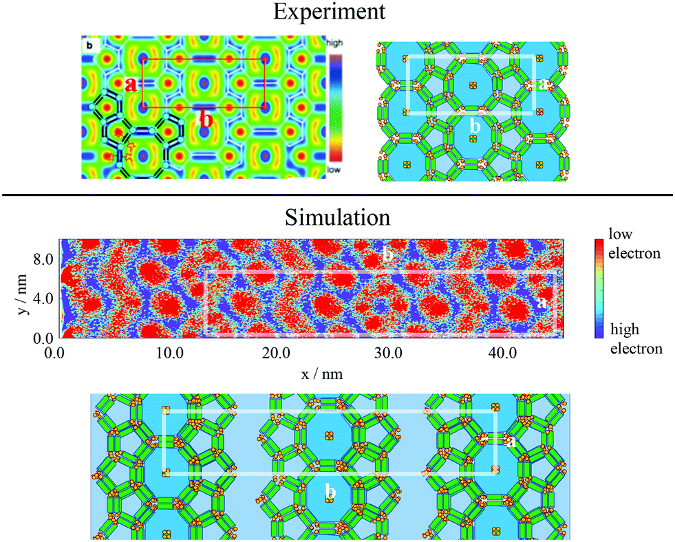
To categorise the phases observed experimentally, Poppe et al.45 generated electron density maps, as well as two-dimensional diffraction patterns using XRD to observe the hexagonal columnar phase (Fig. 10). To compare the snapshots to experimental data, a heatmap of the local mole fraction of the alkyl chain moieties in the plane perpendicular to the director was generated, as well as a 2D diffraction pattern of the alkyl moieties on the same plane. The results are presented in Fig. 10(b) and (d). The simulation results visually match the experimental observations.
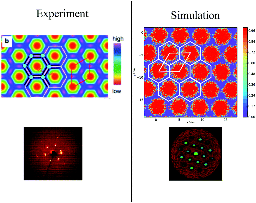 | ||
| Fig. 10 Comparison of experimental and simulations structures: Top Left Electron density map,45 where red and blue are regions of low electron density (i.e. alkyl chains) high electron density (rigid backbone). Top Right Heatmap of local mole fraction of alkyl moieties on the plane perpendicular to the director observed in simulations at T = 380 K, with red and blue highlighting regions of high and low of side-chain density. Bottom Left Diffraction pattern observed experimentally at T = 135 °C (ref. 45). Bottom Right simulated diffraction (T = 400 K). | ||
To calculate the inter-column distance, the planar radial distribution function, g⊥, of the alkyl CG segments was calculated for the plane orthogonal to the director. It was assumed that the value of the first peak corresponds to the inter-columnar distance, and as could be seen in Fig. 11, the simulations predict an inter-columnar distance of 4.2 nm, which agrees with the experimental observations. It is to note that none of the parameters in this work were fitted to the experimental data given by Poppe et al. and therefore this prediction stems from the robustness of the force field parametrisation. The structure factor of the alkyl moiety is also shown in the aforementioned figure, with the peaks having a ratio of 1: :
: :
: :
: clearly indicating a hexagonal ordering.
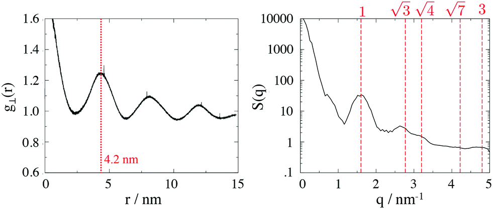 | ||
| Fig. 11 Left Planar radial distribution function, g⊥, of the alkyl moieties on the plane orthogonal to the director. Right Structure factor of the alkyl group in the same system, indicating a hexagonal ordering. | ||
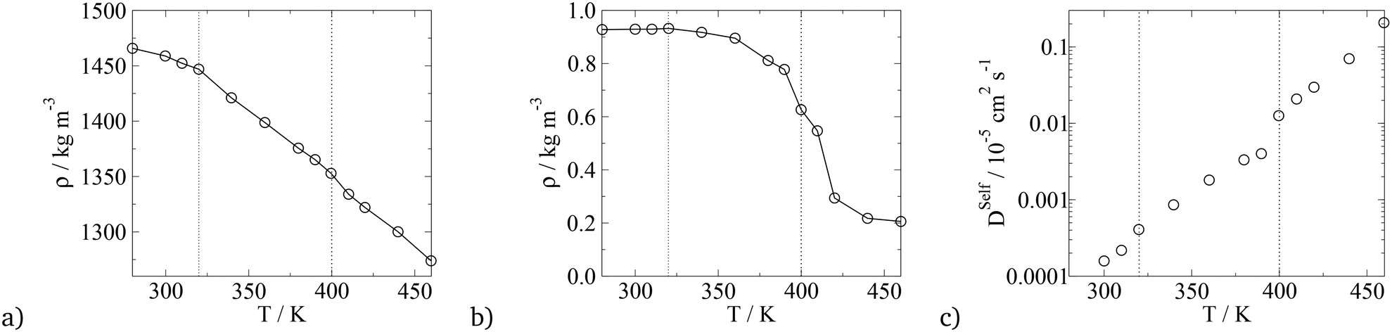
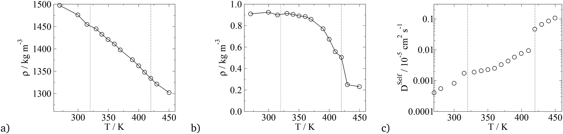
In terms of temperature dependent phase behaviour, it is known from experimental and previous simulation studies that T-shaped bolaamphiphiles have a crystalline solid phase at low temperatures, an isotropic phase behaviour at high temperatures and a liquid crystalline fluid at intermediate temperatures. To investigate this, simulations were run at a range of temperatures from 280 K to 460 K. In order to calculate phase transition temperatures, five parameters were calculated at different temperatures: density, constant volume heat capacity, nematic and orientational planar order parameters as well as the diffusion coefficient of all CG segments. The diagrams can be seen in Fig. 12.
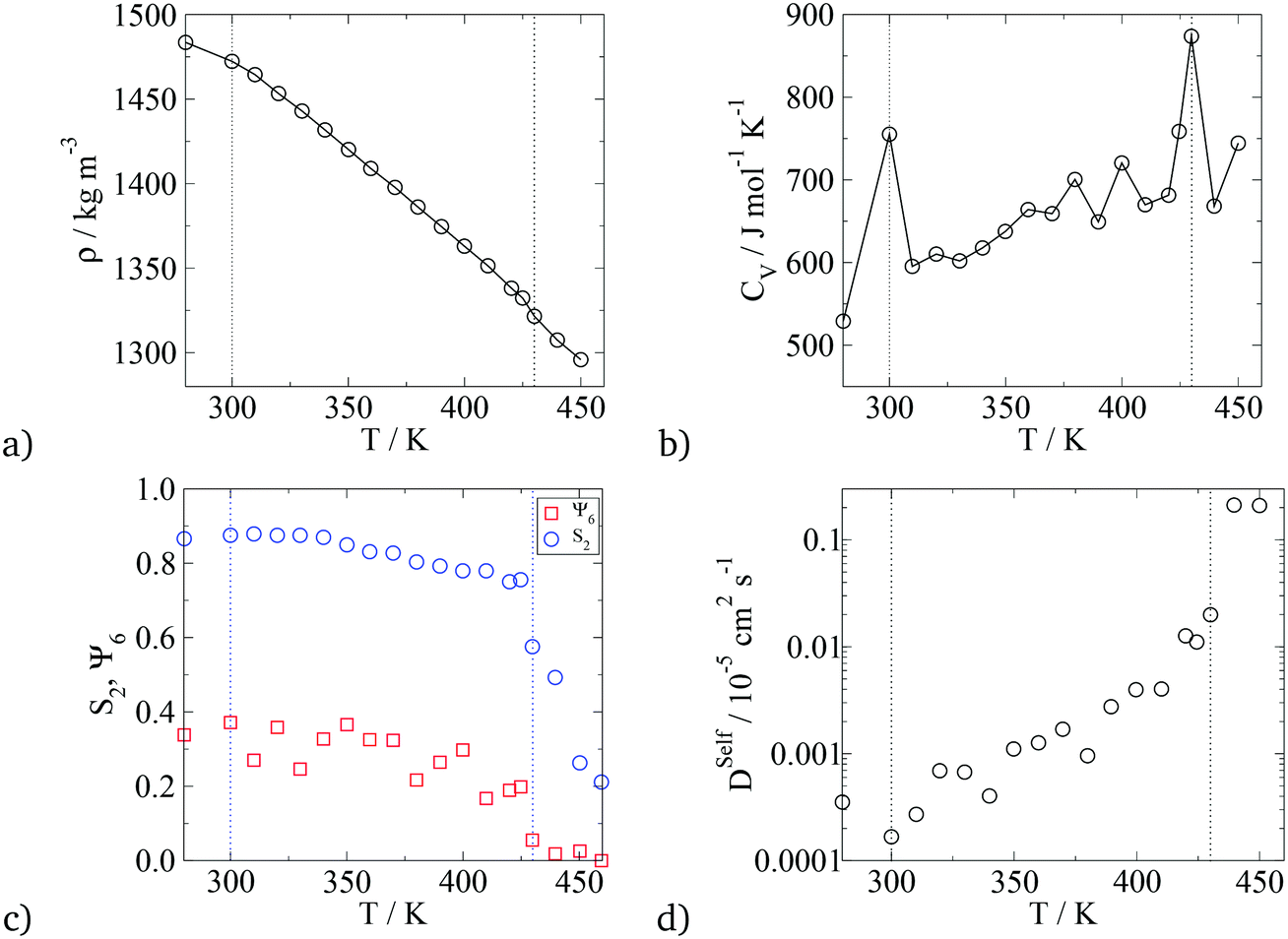 | ||
| Fig. 12 Plots of parameters used to calculate the transition temperature for the T-shaped BA (m = 6, n = 0). a) Density vs. T, b) isochoric heat capacity vs. T, c) nematic order parameter, S2, and the hexagonal orientational planar order parameter, Ψ6, of the principal axis of the rigid backbone vs. T, d) diffusion coefficient of all CG segments vs. T. The dashed lines indicate the crystalline–LC (left) and LC–isotropic (right) transition temperatures. | ||
For all the parameters investigated, there are clear changes in the value of the properties calculated at the onset of phase transition. The phase transitions are most clearly visible in the heat capacity vs. temperature plot where two large peaks are observed at T = 300 K and T = 430 K. At these temperatures, an order of magnitude increase in the diffusion coefficient is observed with increasing temperature by 10 K. This is further backed by the density vs. temperature plots where the slope of the curve changes at T = 300 K and again at T = 430 K, with the change being more pronounced at the lower temperature. These two temperatures are identified as the transition temperatures. The lower transition temperature is the transition from the crystalline solid phase to a liquid crystal, as the diffusion coefficient becomes an order of magnitude higher at T = 320 K than at T = 300 K, but S2 and Ψ6 remain unchanged. This is also seen in Fig. 9, where the histograms at temperatures below 430 K had very similar distributions, with 4 peaks at 0°, 60°, 120° and 180°. At T > 430 K, a flat distribution is observed indicating an isotropic phase. This is commensurate with the sharp drop in the values of the order parameters at T = 430 K, clearly indicating a p6mm–istropic phase transition. The predictions from the simulations as reported here show a very good agreement between this work and the experimental data published by Poppe et al.45 The comparison is presented in Table 6, with the solid–liquid crystal transition temperature being almost the same. The columnar–isotropic phase transition is underestimated by 20 K.
| Phase transition | T Trans, Exp/K | T Trans, Sim/K |
|---|---|---|
| Crystal solid to p6mm Hex Col | 310 | 300 |
| p6mm Hex Col to isotropic | 452 | 430 |
The diffusion coefficient presented in Fig. 12 is the average diffusion in all directions for all segments in the simulation box. Closer analysis of the diffusion coefficient, parallel and perpendicular to the director, clearly indicates faster diffusion along the director. This anisotropy in the value of the diffusion coefficient can be seen in Fig. 13. The lower temperature corresponds to the liquid crystalline system, and the higher temperature to the isotropic system. For the LC phases, the displacements of the molecules parallel to the director are twice as high than displacements perpendicular to it. At 440 K, there is no difference in the value of the diffusivities in different directions, indicating an isotropic phase.
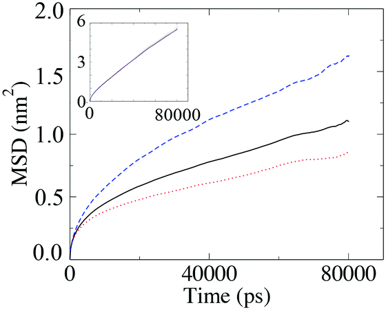 | ||
| Fig. 13 Mean squared displacements of the T-shaped BA molecules parallel and perpendicular to the director at T = 390 K, with the inset being the same plot for T = 440 K where there is no directional differences in diffusion. | ||
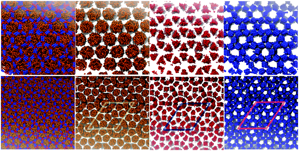
NσT simulations for this molecule were run at different temperatures, with a system composed of 2400 molecules. Equilibrium snapshots at T = 380 K can be seen in Fig. 8(Bottom), exhibiting a large superlattice with a hexagonal p6mm symmetry. To the best of our knowledge, this type of phase behaviour has not been observed in simulation work of polyphilic molecules, be it liquid crystals, surfactants or block copolymers. The columnar phase behaviour can be best understood by looking at the side-chain moiety, depicted using the orange colour in the mentioned figure.
Highlighting the alkyl group, one sees how a central column is surrounded by a disordered ring. This ring is then surrounded by 12 pentagonal columns. This three layered structure forms the basis of the columnar patterns, with these ringed structures forming a hexagonal superlattice. The visual comparison between the predictions of the simulation and the structure observed experimentally is presented in Fig. 14. While similar, the structures are not identical, with the key difference being the number of layers between each central column. In the experimental observations, each central hexagonal column is separated by truncated triangles (non-regular hexagons) formed by three pentagons (Fig. 14(c)). Alternatively this structure can be considered as two rings of pentagons separating the hexagonal columns (see Fig. 14(e)). However, in simulations the distance between every two central columns is three layers, the central one formed by pentagons and the two adjacent representing or the disordered rings. This can be understood more easily using Fig. 14(a) and (b) plotted with the same scale. The radius of the black ring gives the lattice length in experiments, and the white ring gives the lattice length observed in simulations. The lattice length in simulations is clearly an extra layer of pentagons longer.
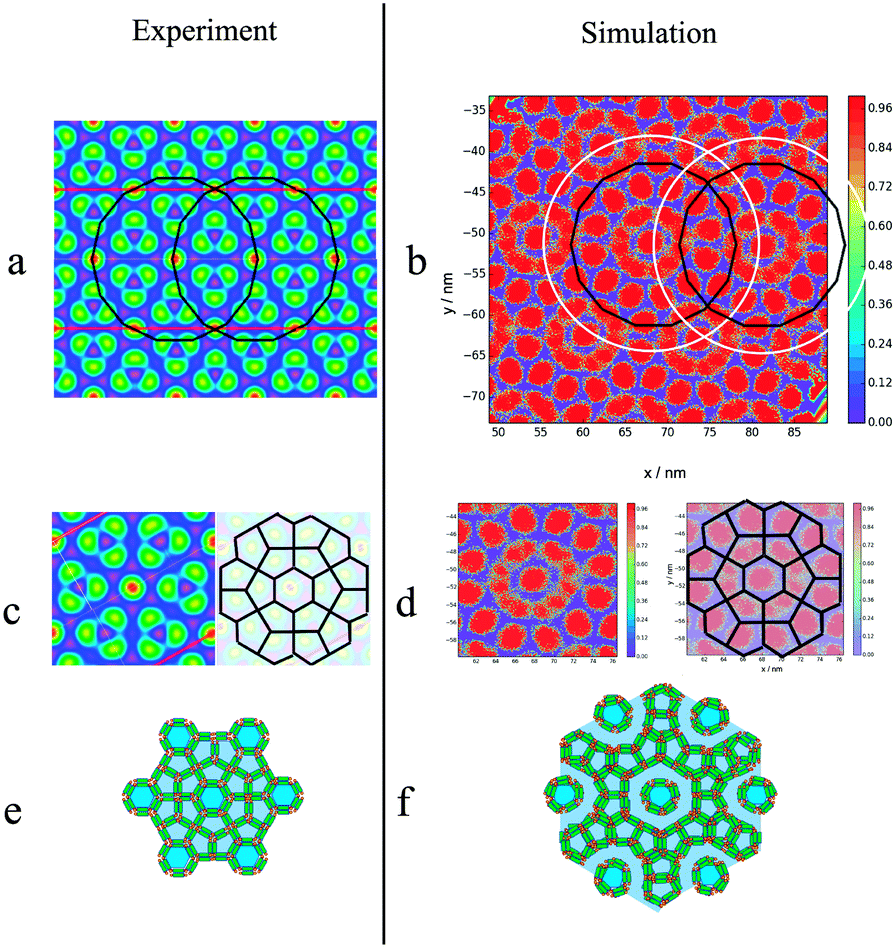 | ||
| Fig. 14 Comparison between structures obtained experimentally and in simulation for the asymmetric BA (m = 5, n = 1): a electron density map taken from ref. 45, with colours explained in Fig. 10. b Heatmap of local mole fraction of alkyl moieties on the plane perpendicular to the director observed in simulations at T = 380 K, with the colours explained in Fig. 10. a and b Have the same scale, with the black and white rings being the distance between the central columns observed experimentally and in simulation respectively. In both cases a hexagonal superlattice is observed with a central hexagonal surrounded by layers of pentagons as highlighted by c–f. | ||
To calculate the lattice length of the hexagonal structure, the planar RDF was calculated for alkyl group, with the fourth peak corresponding to lattice length of the hexagonal columnar phase, as explained in Fig. 14. As also presented in the aforementioned figure, experimentally the third peak of the planar RDF corresponds to the lattice length as only two pentagonal rings separate the central columns from each other. Poppe et al. calculated a lattice length of 9.7 nm, which is in agreement with the distance given by the third peak calculated in this work at 10.1 nm. However, the lattice length in this work was calculated using the fourth peak of the RDF, and was found to be 13.6 nm. The structure factor was also calculated (Fig. 15(c)), with only two peaks being visible, as highlighted in the figure, with the ratios of the peaks (3.82 nm−1:1.94 nm−1) being the same as the ratio of the fourth to the second peak (13.6 nm:6.9 nm) of the RDF. It was not possible to determine any structures from the structure factor. However, the 2D structure factor (i.e. diffraction pattern) shown in Fig. 15(d) clearly shows the twelve peaks corresponding to the twelve pentagons surrounding the central column.
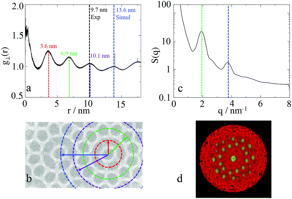 | ||
| Fig. 15
a Planar radial distribution function, g⊥, of the alkyl moieties on the plane orthogonal to the director, with the peaks highlighted with different colours corresponding to distances shown in b. The unit cell distance is 13.1 nm c structure factor of the alkyl group in the same system, with two peaks with a ratio of 2:1 clearly visible, with d showing the 2D diffraction pattern of the same system. | ||
To compare the thermotropic behaviour of the asymmetric BA, simulations were run at different temperatures with the results presented in Fig. 16. For the solid to liquid crystal phase transition, density and the diffusion coefficient were used, and for the LC columnar to isotropic phase transition, the nematic order parameter was used. The comparison between transition temperatures from experiments and simulation is given in Table 7. Experimentally, from 326 to 403 K, an unknown liquid crystalline phase is observed, which is different to the phase discussed. From 403 to 417 K the phase presented in the work is observed and the LC–isotropic phase transition occurs at 417 K. In this work, a crystal to LC phase transition is observed at around 320 K and the p6mm to isotropic phase is observed at 400 K, again the solid–liquid crystal transition temperatures are in quantitative agreement with experiments, however, the LC–isotropic phase transition is underestimated with simulations. It is not discussed in literature what the unknown liquid crystalline phase that is observed in simulations is, however, the quantitative agreement between simulation and experiments is significant. It is also interesting that in this work, as with experiments, the isotropic transition temperature for the swallow-tail BAs is lower than that predicted for the T-shaped BA, signifying that the superlattice phase is less stable at higher temperatures. This could potentially be explained with the help of Fig. 9 in the ESI,† where it is seen that in the LC phase the shorter side chain is confined to the interface between the alkyl groups and the other moieties, which it interacts with unfavourably. In an isotropic system this side chain could interact with more alkyl groups, minimising the unfavourable interactions hence a more stable isotropic phase.
 | ||
| Fig. 16 Plots of parameters used to calculate the transition temperature for the swallow-tail BA (m = 5, n = 1). a) Density vs. T, b) nematic order parameter, S2, and the hexagonal orientational planar order parameter, Ψ6, of the principal axis of the rigid backbone vs. T, c) diffusion coefficient of all CG segments vs. T. The dashed lines indicate the transition temperatures. | ||
| Phase transition | T Trans, Exp/K | T Trans, Sim/K |
|---|---|---|
| Crystalline solid to unknown LC | 326 | — |
| Crystalline solid to p6mm LC | — | 320 |
| Unknown LC to p6mm LC | 403 | — |
| p6mm LC to isotropic | 417 | 400 |
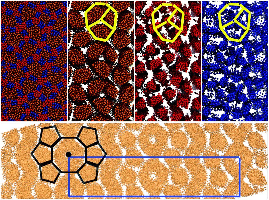 | ||
| Fig. 17 Top The snapshots of different functional groups in the final frame of simulations of 1600 swallow-tail BAs with m = 3, n = 3. Colors are as those as in Fig. 8. The yellow sketch superimposed on the snapshots shows the arrangement of the backbones in the octagonal cells. Bottom Snapshot of the alkyl group with added periodicity to clearly show the c2mm rectangular unit cell, as well as the structure of the octagonal and pentagonal columns. | ||
Comparison between simulations and experimental results is presented in Fig. 18. Sketches are also used to highlight the key difference between the experimentally observed phase and that seen in simulations. In both simulations and experiments there is a row of octagons, surrounded by a row of pentagons on each side. Additionally in simulations there is a zigzag shaped region formed of the alkyl group, with no apparent columnar structure inside the region (i.e. isotropic).
 | ||
| Fig. 18 Comparison between the self-assembly of symmetric swallow-tail BA (m = 3, n = 3) as observed from experiments and simulations. Both experiments and simulation predict a rectangular unit cell columnar phase (c2mm). | ||
To calculate the lattice lengths and compare them to experiments, the mole fraction of the alkyl group on the plane perpendicular to the director was calculated at different points along the director. The mole fractions were then averaged to give a heat map. The lattice lengths were then calculated using the heat map (Fig. 18). Due to the extra disordered alkyl regions present in the simulations, the long side of the unit-cell (denoted as b) was expected to be overestimated. However, the short side (denote as a) is expected to be the same as the experiments. The comparison between the repeat units is given in Table 8. As could be seen, both simulations and experiments give the same lattice length a, at around 6.2 nm. However, the length of the other lattice length b was predicted to be almost twice that of the experimental results.
| Lattice unit | Lengthexp/nm | Lengthsim/nm |
|---|---|---|
| a | 6.2 | 6.2 |
| b | 15.5 | 30.5 |
Finally, the thermotropic properties of the BAs were calculated using the nematic order parameter, the density, and the diffusion coefficient, with the summary of the transition temperatures given in Table 9, with the value of the parameters vs. temperature plotted in Fig. 19. In this work, a crystalline solid phase to a liquid crystalline phase is characterised by the change in the diffusion coefficient and the drop in the density, which occurs around 315 K. The simulations underestimate this transition temperature by almost 30 K. However, the LC–isotropic transition temperature is predicted correctly using the nematic S2 order parameter.
| Phase transition | T Trans, Exp/K | T Trans, Sim/K |
|---|---|---|
| Crystalline solid to c2mm | 348 | 315 |
| c2mm to isotropic | 420 | 420 |
 | ||
| Fig. 19 Plots of parameters used to calculate the transition temperature, for the swallow-tail BA (m = 3, n = 3). a) Density vs. T, b) Nematic order parameter, S2, and the hexagonal orientational planar order parameter, Ψ6, of the principal axis of the rigid backbone vs. T, c) diffusion coefficient of all CG segments vs. T. The dashed lines indicate the transition temperatures. | ||
4 Conclusions
In this study, a robust method of coarse-graining complex polyphilic bolaamphiphiles was presented improving upon previous phenomenological simulation studies of these molecules. The key highlight is the use of force field parameters derived using the SAFT-γ Mie methodology. It was shown that the force field parameters correctly predict the key features of the recently discovered structures for of medium chain swallow-tailed BAs. From the experimental point of view, these simulations can aid to better understand the structure of the mesophases, as has been demonstrated in our analysis of the arrangement of the BA molecules in the c2mm phase (octagonal and pentagonal columns). Furthermore, the SAFT force field has the ability to predict the correct dimensions as well as the transition temperatures for the system studied.Conflicts of interest
There are no conflicts to declare.Acknowledgements
The authors acknowledge, thank and appreciate the rich input, suggestions and comments to this manuscript made by Prof. Carsten Tschierske. E. A. M. acknowledges the support from EPSRC through research grants to the Molecular Systems Engineering group (grant no. EP/E016340, EP/J014958, and EP/R013152). M. F. T. acknowledges the support of the Department of Chemical Engineering, Imperial College London through a departmental scholarship. Computations were performed employing the resources of Imperial College Research Computing Service (DOI: 10.14469/hpc/2232) and the UK Materials and Molecular Modelling Hub, which is partially funded by EPSRC (grant no. EP/P020194).Notes and references
- G. M. Whitesides, J. P. Mathias and C. T. Seto, Molecular self-assembly and nanochemistry: a chemical strategy for the synthesis of nanostructures, Dtic document technical report, 1991 Search PubMed.
- L. F. Lindoy and I. M. Atkinson, Self-assembly in supramolecular systems, Royal Society of Chemistry, 2000 Search PubMed.
- S. Glotzer, M. Solomon and N. A. Kotov, AIChE J., 2004, 50, 2978–2985 Search PubMed.
- C. Tschierske, Angew. Chem., Int. Ed., 2013, 52, 8828–8878 Search PubMed.
- P. F. Damasceno, M. Engel and S. C. Glotzer, Science, 2012, 337, 453–457 Search PubMed.
- V. Polshettiwar, B. Baruwati and R. S. Varma, ACS Nano, 2009, 3, 728–736 Search PubMed.
- M. D. Pluth, R. G. Bergman and K. N. Raymond, Acc. Chem. Res., 2009, 42, 1650–1659 Search PubMed.
- C. T. Black, R. Ruiz, G. Breyta, J. Y. Cheng, M. E. Colburn, K. W. Guarini, H.-C. Kim and Y. Zhang, IBM J. Res. Dev., 2007, 51, 605–633 Search PubMed.
- J. Van Haaren and D. Broer, Chem. Ind., 1998, 24, 1017–1021 Search PubMed.
- J.-H. Fuhrhop and T. Wang, Chem. Rev., 2004, 104, 2901–2938 Search PubMed.
- A. J. Crane, Ph.D. Thesis, Imperial College London, 2010 Search PubMed.
- E. de Miguel and C. Vega, J. Chem. Phys., 2002, 117, 6313–6322 Search PubMed.
- T. van Westen, B. Oyarzún, T. J. Vlugt and J. Gross, J. Chem. Phys., 2015, 142, 244903 Search PubMed.
- P. Bolhuis and D. Frenkel, J. Chem. Phys., 1997, 106, 666–687 Search PubMed.
- B. Oyarzún, T. van Westen and T. J. Vlugt, J. Chem. Phys., 2013, 138, 204905 Search PubMed.
- F. Hentrich, C. Tschierske, S. Diele and C. Sauer, J. Mater. Chem., 1994, 4, 1547–1558 Search PubMed.
- M. Kölbel, T. Beyersdorff, X. H. Cheng, C. Tschierske, J. Kain and S. Diele, J. Am. Chem. Soc., 2001, 123, 6809–6818 Search PubMed.
- M. Prehm, C. Enders, M. Y. Anzahaee, B. Glettner, U. Baumeister and C. Tschierske, Chem. – Eur. J., 2008, 14, 6352–6368 Search PubMed.
- X. Cheng, M. Prehm, M. K. Das, J. Kain, U. Baumeister, S. Diele, D. Leine, A. Blume and C. Tschierske, J. Am. Chem. Soc., 2003, 125, 10977–10996 Search PubMed.
- X. Cheng, M. K. Das, U. Baumeister, S. Diele and C. Tschierske, J. Am. Chem. Soc., 2004, 126, 12930–12940 Search PubMed.
- X. Cheng, F. Liu, X. Zeng, G. Ungar, J. Kain, S. Diele, M. Prehm and C. Tschierske, J. Am. Chem. Soc., 2011, 133, 7872–7881 Search PubMed.
- B. Glettner, F. Liu, X. Zeng, M. Prehm, U. Baumeister, G. Ungar and C. Tschierske, Angew. Chem., Int. Ed., 2008, 47, 6080–6083 Search PubMed.
- M. Prehm, F. Liu, U. Baumeister, X. Zeng, G. Ungar and C. Tschierske, Angew. Chem., Int. Ed., 2007, 46, 7972–7975 Search PubMed.
- F. Liu, M. Prehm, X. Zeng, C. Tschierske and G. Ungar, J. Am. Chem. Soc., 2014, 136, 6846–6849 Search PubMed.
- X. Zeng, M. Prehm, G. Ungar, C. Tschierske and F. Liu, Am. Ethnol., 2016, 128, 8464–8467 Search PubMed.
- B. Chen, X. Zeng, U. Baumeister, G. Ungar and C. Tschierske, Science, 2005, 307, 96–99 Search PubMed.
- R. Kieffer, M. Prehm, K. Pelz, U. Baumeister, F. Liu, H. Hahn, H. Lang, G. Ungar and C. Tschierske, Soft Matter, 2009, 5, 1214–1227 Search PubMed.
- C. Tschierske, C. Nürnberger, H. Ebert, B. Glettner, M. Prehm, F. Liu, X.-B. Zeng and G. Ungar, Interface Focus, 2012, 2, 669–680 Search PubMed.
- G. Ungar, C. Tschierske, V. Abetz, R. Holyst, M. A. Bates, F. Liu, M. Prehm, R. Kieffer, X. Zeng and M. Walker, et al. , Adv. Funct. Mater., 2011, 21, 1296–1323 Search PubMed.
- X. Zeng, R. Kieffer, B. Glettner, C. Nürnberger, F. Liu, K. Pelz, M. Prehm, U. Baumeister, H. Hahn and H. Lang, et al. , Science, 2011, 331, 1302–1306 Search PubMed.
- T. Kong, J. Hu, Y. Xiao, C. Liu and X. Cheng, ChemistrySelect, 2019, 4, 10674–10680 Search PubMed.
- A. J. Crane and E. A. Müller, Faraday Discuss., 2010, 144, 187–202 Search PubMed.
- D. Reith, M. Pütz and F. Müller-Plathe, J. Comput. Chem., 2003, 24, 1624–1636 Search PubMed.
- T. C. Moore, C. R. Iacovella and C. McCabe, J. Chem. Phys., 2014, 140, 224104 Search PubMed.
- T. D. Potter, J. Tasche and M. R. Wilson, Phys. Chem. Chem. Phys., 2019, 21, 1912–1927 Search PubMed.
- C.-C. Fu, P. M. Kulkarni, M. S. Shell and L. G. Leal, J. Chem. Phys., 2012, 137, 164106 Search PubMed.
- S. Izvekov and G. A. Voth, J. Phys. Chem. B, 2005, 109, 2469–2473 Search PubMed.
- M. S. Shell, Adv. Chem. Phys., 2016, 161, 395–441 Search PubMed.
- S. J. Marrink, H. J. Risselada, S. Yefimov, D. P. Tieleman and A. H. De Vries, J. Phys. Chem. B, 2007, 111, 7812–7824 Search PubMed.
- P. C. Souza, R. Alessandri, J. Barnoud, S. Thallmair, I. Faustino, F. Grünewald, I. Patmanidis, H. Abdizadeh, B. M. Bruininks and T. A. Wassenaar, et al. , Nat. Methods, 2021, 1–7 Search PubMed.
- E. A. Müller and G. Jackson, Annu. Rev. Chem. Biomol. Eng., 2014, 5, 405–427 Search PubMed.
- A. J. Crane, F. J. Martínez-Veracoechea, F. A. Escobedo and E. A. Müller, Soft Matter, 2008, 4, 1820–1829 Search PubMed.
- A. J. Crane and E. A. Müller, J. Phys. Chem. B, 2011, 115, 4592–4605 Search PubMed.
- J. D. Weeks, D. Chandler and H. C. Andersen, J. Chem. Phys., 1971, 54, 5237–5247 Search PubMed.
- S. Poppe, A. Lehmann, A. Scholte, M. Prehm, X. Zeng, G. Ungar and C. Tschierske, Nat. Commun., 2015, 6, 8637 Search PubMed.
- M. A. Bates and M. Walker, Phys. Chem. Chem. Phys., 2009, 11, 1893–1900 Search PubMed.
- M. Bates and M. Walker, Soft Matter, 2009, 5, 346–353 Search PubMed.
- M. A. Bates and M. Walker, Liq. Cryst., 2011, 38, 1749–1757 Search PubMed.
- M. A. Bates and M. Walker, Mol. Cryst. Liq. Cryst., 2010, 525, 204–211 Search PubMed.
- X. Liu, K. Yang and H. Guo, J. Phys. Chem. B, 2013, 117, 9106–9120 Search PubMed.
- F. Liu, P. Tang, H. Zhang and Y. Yang, Macromolecules, 2018, 51, 7807–7816 Search PubMed.
- Y. Sun, P. Padmanabhan, M. Misra and F. A. Escobedo, Soft Matter, 2017, 13, 8542–8555 Search PubMed.
- C. Herdes, E. Santiso, C. James, J. Eastoe and E. A. Müller, J. Colloid Interface Sci., 2015, 45, 16–23 Search PubMed.
- G. Jiménez-Serratos, T. S. Totton, G. Jackson and E. A. Müller, J. Phys. Chem. B, 2019, 123, 2380–2396 Search PubMed.
- G. Jiménez-Serratos, C. Herdes, A. J. Haslam, G. Jackson and E. A. Müller, Macromolecules, 2017, 50, 4840–4853 Search PubMed.
- J. Tasche, E. F. Sabattieé, R. L. Thompson, M. Campana and M. R. Wilson, Macromolecules, 2020, 53, 2299–2309 Search PubMed.
- A. K. Pervaje, C. C. Walker and E. E. Santiso, Mol. Simul., 2019, 45, 1223–1241 Search PubMed.
- C. C. Walker, J. Genzer and E. E. Santiso, J. Chem. Phys., 2019, 150, 034901 Search PubMed.
- T. D. Potter, J. Tasche, E. L. Barrett, M. Walker and M. R. Wilson, Liq. Cryst., 2017, 44, 1979–1989 Search PubMed.
- C. Herdes, T. S. Totton and E. A. Müller, Fluid Phase Equilib., 2015, 406, 91–100 Search PubMed.
- V. Papaioannou, T. Lafitte, C. Avendaño, C. S. Adjiman, G. Jackson, E. A. Müller and A. Galindo, J. Chem. Phys., 2014, 140, 054107 Search PubMed.
- P. Hutacharoen, S. Dufal, V. Papaioannou, R. M. Shanker, C. S. Adjiman, G. Jackson and A. Galindo, Ind. Eng. Chem. Res., 2017, 56, 10856–10876 Search PubMed.
- S. Nosé, Mol. Phys., 1984, 52, 255–268 Search PubMed.
- W. G. Hoover, Phys. Rev. A: At., Mol., Opt. Phys., 1985, 31, 1695 Search PubMed.
- M. Parrinello and A. Rahman, J. Appl. Phys., 1981, 52, 7182–7190 Search PubMed.
- M. J. Abraham, T. Murtola, R. Schulz, S. Páll, J. C. Smith, B. Hess and E. Lindahl, SoftwareX, 2015, 1, 19–25 Search PubMed.
- A. Saupe, Angew. Chem., Int. Ed. Engl., 1968, 7, 97–112 Search PubMed.
- M. P. Allen, G. T. Evans, D. Frenkel and B. Mulder, Adv. Chem. Phys., 1993, 86, 1–166 Search PubMed.
- R. J. Low, Eur. J. Phys., 2002, 23, 111 Search PubMed.
- C. Avendaño and E. A. Müller, Soft Matter, 2011, 7, 1694–1701 Search PubMed.
- M. P. Allen and D. J. Tildesley, Computer simulation of liquids, Oxford university press, 2nd edn, 2017 Search PubMed.
- W. Humphrey, A. Dalke and K. Schulten, J. Mol. Graphics, 1996, 14, 33–38 Search PubMed.
- P. J. Linstrom and W. G. Mallard, J. Chem. Eng. Data, 2001, 46, 1059–1063 Search PubMed.
- A. Mejía, C. Herdes and E. A. Müller, Ind. Eng. Chem. Res., 2014, 53, 4131–4141 Search PubMed.
- V. Papaioannou, F. Calado, T. Lafitte, S. Dufal, M. Sadeqzadeh, G. Jackson, C. S. Adjiman and A. Galindo, Fluid Phase Equilib., 2016, 416, 104–119 Search PubMed.
- S. Rahman, O. Lobanova, G. Jiménez-Serratos, C. Braga, V. Raptis, E. A. Müller, G. Jackson, C. Avendaño and A. Galindo, J. Phys. Chem. B, 2018, 122, 9161–9177 Search PubMed.
- M. G. Martin and J. I. Siepmann, J. Phys. Chem. B, 1998, 102, 2569–2577 Search PubMed.
- J. M. Stubbs, J. J. Potoff and J. I. Siepmann, J. Phys. Chem. B, 2004, 108, 17596–17605 Search PubMed.
- W. L. Jorgensen, D. S. Maxwell and J. Tirado-Rives, J. Am. Chem. Soc., 1996, 118, 11225–11236 Search PubMed.
Footnote |
| † Electronic supplementary information (ESI) available. See DOI: 10.1039/d1me00021g |
| This journal is © The Royal Society of Chemistry 2021 |