
 Open Access Article
 This Open Access Article is licensed under a
 Creative Commons Attribution 3.0 Unported Licence
Feasibility of graphene–polymer composite membranes for forward osmosis applications†
Sevilay
Akca
 ab,
Pınar
Arpaçay
ac,
Niall
McEvoy
d,
Oleg
Prymak
e,
Werner J.
Blau
*a and
Mathias
Ulbricht
*b
ab,
Pınar
Arpaçay
ac,
Niall
McEvoy
d,
Oleg
Prymak
e,
Werner J.
Blau
*a and
Mathias
Ulbricht
*b
aSchool of Physics, The Centre for Research on Adaptive Nanostructures and Nanodevices (CRANN), and Advanced Materials and BioEngineering Research (AMBER) Centre, Trinity College Dublin, Dublin 2, Ireland. E-mail: wblau@tcd.ie
bLehrstuhl für Technische Chemie II and Center for Nanointegration Duisburg-Essen (CENIDE), Universität Duisburg-Essen, 45141 Essen, Germany. E-mail: mathias.ulbricht@uni-essen.de
cInstitute of Nanotechnology and Institute of Quantum Materials and Technology, Karlsruhe Institute of Technology (KIT), P.O. Box 3640, 76021 Karlsruhe, Germany
dAdvanced Materials and Bioengineering Research (AMBER) Centre & School of Chemistry, Trinity College Dublin, Dublin, Ireland
eInorganic Chemistry and Center for Nanointegration Duisburg-Essen (CENIDE), University Duisburg-Essen, 45141 Essen, Germany
First published on 15th September 2021
Abstract
This paper assesses the feasibility of fabricating thin-film composite membranes from stacked graphene nanosheets in combination with a polymer as a selective layer on a macroporous support membrane for utilization in osmosis applications. Reproducible dispersion procedures based on the liquid-phase exfoliation technique have been established to fabricate multi-layer graphene from graphite with the assistance of the high boiling point solvent N-methylpyrrolidone (NMP) or the low boiling point solvent ethanol. A high graphene yield of up to 7.2% with a concentration of 0.36 mg mL−1 was achieved in the NMP-based dispersions. Membrane fabrication toward a graphene–polymer sandwich architecture has been developed, in which graphene laminates modified with or without a chemical cross-linker are placed in between two polyethyleneimine (PEI layers) laminated onto the support membrane (either nylon or polyethersulfone microfiltration membranes). Graphene–polymer composite membranes were successfully fabricated via the pressure-assisted filtration technique and the performance of the membranes was studied in terms of pure water permeability and dextran rejection. The best performing membranes had water permeability varying from 33–77 L m−2 h−1 bar−1 and rejection of dextran 2000 kDa up to 96%; the selective layer has a thickness of ∼1 μm. Forward osmosis experiments with polyacrylic acid sodium salt as draw agent demonstrate the feasibility of using the established graphene-polymer composite membranes for such applications.
1. Introduction
Graphene is one-atom thick, an individual two-dimensional (2D) layer consisting of covalently-bonded carbon atoms arranged in a honeycomb lattice. Graphite consists of graphene sheets which are stacked on each other into a 3D structure and connected by weak van der Waals interaction. The interlayer distance of these sheets is approximately 3.4 Å.1 Graphene has been widely studied due to its extraordinary properties including its high values of Young's modulus, strength, thermal conductivity, charge-carrier mobility and specific surface area. The exceptional properties of graphene and its derivatives continue to attract intense research interest in many processes and applications.2–4 One-atom thickness and nearly frictionless surface make graphene the ultimate material in membrane separation technology,5,6 because of the inverse relationship between membrane permeance and membrane thickness.There are some limitations in the current separation membranes, such as difficulty in tuning water and solute permeability, low fouling/chemical resistance, etc. It has been underlined that there is a significant necessity of designing new generation membranes with solid and engineered pore structure, scalable for practical modules.7 More recently, researchers have been examining 2D graphene as building blocks for separation membranes, leading to exciting improvements based on exceptional separation mechanism and leading to potentially very high separation performance.8–12 Enormous effort has been focused on the production of graphene to search for a cost-effective method which will provide defect-free graphene on a large scale. The liquid-phase exfoliation technique (LPE) has been considered as the most versatile method for graphene production due to its capability of mass production. Furthermore, it is a straightforward and scalable process. There are different types of exfoliation processes which include two popular examples. The first example is oxidation of graphite to give graphene oxide (GO)13 and the second example is sonication-assisted exfoliation of graphite that is stabilized by using carefully selected solvents or surfactants.14 One advantage of graphene oxide dispersions is that they mainly consist of monolayer flakes. However, the oxidation process can also be a disadvantage due to the introduction of structural defects15,16 that alter the physical properties of graphene. Sonication-assisted LPE can provide defect-free flakes but with a comparatively low monolayer content.17 LPE consists of three major steps. First, it is essential to choose an appropriate solvent to disperse pristine graphite, which will overcome the van der Waals interaction between adjacent layers held within a π–π stacking distance of ∼3.4 Å. Energy provided through sonication or shear force assists in separating individual platelets from the pristine graphite. Furthermore, since graphene flakes tend to reaggregate within a certain time, a strong solvent–solute interaction is necessary to stabilize the graphene nanosheets in the dispersion for a long time by balancing inter-sheet attractive forces.18 The produced dispersion after sonication is expected to be highly poly-dispersed;19 in the final step, a size selection process is performed by mild centrifugation. Unexfoliated large graphitic structures in the suspension are removed from the well-exfoliated smaller flakes by centrifugation.
The dispersibility of such materials in a solvent can be categorized by various models for instance; surface energy, Hildebrand-20 and Hansen-21based solubility models. According to the surface-energy-based model, solvents which have a surface energy of ∼40 mJ m−2 are considered as the best candidates for the dispersion of graphitic structures, because they minimize the interfacial tension between the solvent and graphene.18 However, most of the best solvents with a surface energy of ∼40 mJ m−2, such as NMP (40 mJ m−2), dimethylformamide (37.1 mJ m−2) and ortho-dichlorobenzol (37 mJ m−2),22 have crucial drawbacks. These solvents are not user-friendly due to their toxicity (they can be absorbed by the skin and damage organs), potential negative environmental impacts and high boiling point. Herein, low-boiling-point organic solvent-based dispersions are employed as an alternative to high-boiling point organic solvents. However, the solubility of graphite in low-boiling point solvents is poor, typically resulting in very low dispersion efficiency. According to literature, graphene can be fabricated via exfoliation of graphite in ethanol-based liquids with a concentration of only ∼0.002 mg mL−1 in pure ethanol, and 0.014 mg mL−1 in water–ethanol mixture.23,24 An improvement in the dispersion efficiency in ethanol, yielding up to 0.5 mg mL−1 for few-layered graphene, was achieved using a drastically long sonication process, for about 300 h.25 In order to improve the solubility of graphite in ethanol, a promising exfoliation method assisted with salt as an intercalator is proposed in the current work. Here, the function of the organic salt (potassium sodium tartrate, KNaC4H4O6·4H2O) in the dispersion is to be intercalated into the graphite interlayer spaces and, thus, to expand the spacing of the graphitic layers, resulting in weakened van der Waals forces and improving the electrical repulsion between the sheets.
Graphene nanosheets can be assembled into highly-ordered, stacked graphene laminates on a porous substrate via pressure-assisted filtration assembly. Multi-layer, well-packed graphene laminates allow water to pass but reject other molecules. The pure graphene, without functional groups, provides frictionless carbon walls, which are the basis of fast, friction-less, transport of water.26,27 Two typical transport mechanisms28 can occur in such membranes, i.e. either through interlayer channels between flakes or through structural defects within graphene flakes. The defects must be identified and eliminated from such stacked-graphene-nanosheet membranes in order to enhance the sieving properties. Sealing or blocking defects29 is one way to enhance the transport selectivity. This work aimed to fabricate graphene composite membrane without any application of excessive oxidation during graphene production. By this way, physical properties of graphene were preserved by eliminating the introduction of structural defects during oxidation. Most of the works in the field of graphene-based membranes follow the way of producing GO which is chemically modified graphene fabricated by various oxidative modification techniques; such as Hummers' method. After that, reduction-based approach by solution (hydrazine hydrate) and thermal methods are applied to reduce oxygenic functional groups.
Forward osmosis (FO) can be described as water transport across a selectively permeable membrane, which is driven by an osmotic pressure difference, from a solution with high water chemical potential (feed solution) to a solution with low water chemical potential (draw solution).30 This transport will proceed until the chemical potential across the membrane arrives at the equilibrium level. FO is applicable to a wide range of fields such as desalination, power generation, wastewater treatment, drug and food industry. Osmotically driven membrane processes including FO attracted a great attention across the world owing to their energy efficiency and because they are less prone to membrane fouling.31 It provides sustainable solutions against water and energy scarcity. Nevertheless, the absence of suitable FO membranes with effective separation performance is the main drawback. Use of nanotechnology for fabrication of the membrane is one of most common methods to enhance the separation performance.32 An ideal FO membrane should fulfil the following requirements;33 (i) high salt retention and high water flux; (ii) low concentration polarization; and (iii) high long-term chemical, mechanical and performance stability. A thin permeation-selective active layer on a thin support layer with optimum porosity to reduce internal concentration polarization (ICP), high hydrophilicity and low fouling tendency would be desirable for such materials.30
The draw solute has a significant effect on the efficiency of the FO performance. Recently, a remarkable amount of effort has been devoted to exploring the ideal draw agent which should fulfil the following characteristics; (i) high osmotic pressure which creates high water flux; (ii) low reverse solute transport through the membrane; (iii) easy recovery of the diluted draw solution after FO; and (iv) nontoxic and cost-friendly.34 Many possible candidates have been discussed such as organic ionic salts35 and organic compounds,36etc. However, in recent years another draw solute candidate has been discovered from the commercially available, and potentially also pH-responsive, polymer family called polyelectrolytes.37–39 Polyelectrolytes possess many unique properties which make them suitable as draw solutes for osmotic processes. Specifically, polyacrylic acid sodium salts (PAA-Na) have been found to be an appropriate option, since they are water-soluble polymers available with different molecular weights, they have a capacity to produce high osmotic pressures and they can induce high water flux with low reverse solute flux due to their expanded colloid size.39 Furthermore, their macromolecular sizes allow them to be recycled easily from diluted draw solution by using low-pressure, low-energy ultrafiltration processes.
In the present study; in order to fabricate graphene–polymer composite membranes, multi-layer graphene produced via the liquid-phase exfoliation method is used as the building block to fabricate a sandwich-like graphene–polymer hybrid layer laminated to the macroporous support membrane by using the pressure-assisted filtration technique (Fig. 1). Firstly, microfilter support membranes are coated with a positively charged polymer, polyethyleneimine (PEI), in order to improve the bond between the surface of the support and the graphene flakes (due to the negatively charged nature of the support membrane and using interactions with carboxyl groups on the graphene, either as defects or due to adsorbed tartrate) and also increase membrane selectivity. Secondly, graphene is deposited and, with the aim of enhancing the stability and stacking quality of graphene laminates in aqueous phases, a chemical cross-linker, ethylenediamine (EDA) that is dissolved in the graphene dispersion in order to introduce covalent bonds between functional groups (e.g. carboxyl) on the graphene is also evaluated (Fig. 1b), compared to deposition in the absence of cross-linker (Fig. 1a). Even though, cross-linking can provide the membranes with enough stability in water, an effective strategy should be to introduce an optimum amount of cross-linker. Excessive cross-linking might cause a decrease of the water flux of the membrane. In the current work, various proportions of EDA were studied to study its effect on stability, water permeability and rejection characteristics of the membranes. Finally, a second layer of PEI is applied in order to increase the membrane stability and selectivity. In this work, the terms of ‘hybrid’ and ‘composite’ are used for the active layer (i.e., graphene and polymer structure) and for the combination of the active layer with the support membrane, respectively.
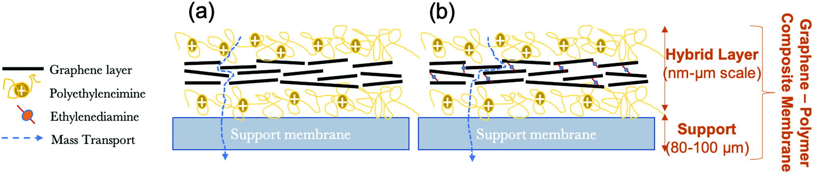 | ||
| Fig. 1 Schematic diagram of graphene–polymer composite membranes in the absence of cross-linker (a) and in the presence of cross-linker (b). | ||
The prepared membranes are expected to have a good performance in the ultrafiltration range (high water flux and macromolecule rejection) and feasibility for FO applications with macromolecular draw agents such as PAA-Na. A series of parameter variations and structural characterizations are conducted to understand the quality of produced graphene dispersions and to determine the most suitable composite membrane preparation conditions. Resulting compositions and structures of graphene-based membranes are analysed and discussed. Finally, FO tests are carried out to assess the performance of a prototype graphene–polymer hybrid membrane.
2. Experimental section
2.1. Materials
Ethanol (absolute, 99.5%, Acros Organics) was purchased from Thermo Fisher Scientific and N-methyl-2-pyrrolidone (NMP) was obtained from Merck Millipore KGaA (Germany). Potassium sodium tartrate (KNaC4H4O6·4H2O; ACS reagent, 99%), poly(ethyleneimine) (PEI; average Mw ∼ 750![[thin space (1/6-em)]](https://www.rsc.org/images/entities/char_2009.gif) 000 g mol−1, ∼50% in H2O), ethylenediamine (EDA), and poly(acrylic) acid sodium salt (PAA-Na; with different molecular weights nominal Mw ∼ 5100 g mol−1; Mw ∼ 8000 g mol−1, 45 wt% in H2O and Mw ∼ 30000 g mol−1, 40 wt% in H2O) were supplied by Sigma-Aldrich. For the analysis of membrane selectivity, various molecular weights (4 kDa and 2000 kDa) of dextran were used and supplied from Sigma Aldrich. Graphite (+100 mesh ≥ 75%) was purchased from Sigma-Aldrich. The porous support membranes (47 mm diameter disks) made from nylon and polyethersulfone (PES) were from Supelco and Sartorius. The average pore sizes of porous support membranes were characterized by the method of gas flow/pore dewetting permporometry and specified as 0.27 μm for nylon and 0.12 μm for PES. Silicon wafers (SiO2, oxide thickness: 285 nm; wafer thickness: 525 micron) were purchased from Graphene Supermarket. Holey carbon grids (400 mesh) were bought from Agar Scientific Ltd, UK. Graphene fabrication tools are listed as follows: ultrasonic bath (Elmasonic Transsonic, TI-H-10), ultrasonic probe (Sonopuls HD 2200 ultrasonic laboratory homogenizer, Bandelin), centrifuge (Hettich Universal 320) and ultrahigh centrifuge (Thermo electron corporation, Sorvall WX Ultra Series).
000 g mol−1, ∼50% in H2O), ethylenediamine (EDA), and poly(acrylic) acid sodium salt (PAA-Na; with different molecular weights nominal Mw ∼ 5100 g mol−1; Mw ∼ 8000 g mol−1, 45 wt% in H2O and Mw ∼ 30000 g mol−1, 40 wt% in H2O) were supplied by Sigma-Aldrich. For the analysis of membrane selectivity, various molecular weights (4 kDa and 2000 kDa) of dextran were used and supplied from Sigma Aldrich. Graphite (+100 mesh ≥ 75%) was purchased from Sigma-Aldrich. The porous support membranes (47 mm diameter disks) made from nylon and polyethersulfone (PES) were from Supelco and Sartorius. The average pore sizes of porous support membranes were characterized by the method of gas flow/pore dewetting permporometry and specified as 0.27 μm for nylon and 0.12 μm for PES. Silicon wafers (SiO2, oxide thickness: 285 nm; wafer thickness: 525 micron) were purchased from Graphene Supermarket. Holey carbon grids (400 mesh) were bought from Agar Scientific Ltd, UK. Graphene fabrication tools are listed as follows: ultrasonic bath (Elmasonic Transsonic, TI-H-10), ultrasonic probe (Sonopuls HD 2200 ultrasonic laboratory homogenizer, Bandelin), centrifuge (Hettich Universal 320) and ultrahigh centrifuge (Thermo electron corporation, Sorvall WX Ultra Series).
2.2. Methods
| Solvent | Dispersion | Sonication type | Sonication time (h) | Centrifugation speed (rpm) | Centrifugation time (min) | Number of centrifugation steps |
|---|---|---|---|---|---|---|
| NMP | N1 | Sonic probe | 4 | 1500 | 45 | 1 |
| N2 | Sonic probe | 4 | 4500 | 45 | 1 | |
| N3 | Sonic probe | 4 | 4500 | 45 | 2 | |
| Ethanol | E1 | Sonic bath | 5 | 3000 | 30 | 1 |
| E2 | Sonic bath | 5 | 3000 | 30 | 2 |
:EDA; 1:15, 1:1200, 1:15000) and the mixture was allowed for about 1 h for chemical reaction) – or without cross-linked was filtrated through the PEI-modified membrane.
After completing the graphene deposition, the wet membranes were immediately dried at 50 °C for 2 hours to improve the strength of graphene and PEI and remove the excessive solvent residuals. Thirdly, a second PEI coating on the top (with the same protocol mentioned above) was applied to the prepared modified membrane followed by drying in a vacuum oven at 50 °C for 1 hour. Then, the membranes were soaked in water overnight to remove unbonded PEI before filtration experiments. In the present work, graphene–polymer composite membranes are labelled as shown in the following:
| Support membrane/(PEIx/Gy/PEIz) and support membrane/(PEIx/Gy + EDAk/PEIz). |
2.3. Characterization
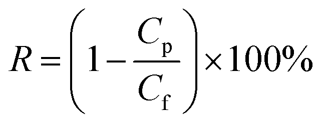
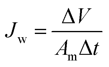
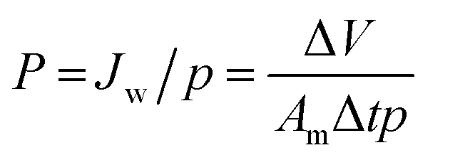 | (1) |
 | (2) |
 | (3) |
The reverse solute leakage (Js, g m−2 h−1), was determined from concentration change of the feed solution in a certain time interval according to:
 | (4) |
3. Results and discussion
3.1. Graphene dispersions
Dispersions were prepared using parameters outlined in Table 1. Fig. 2A and B display the absorption spectra of graphene dispersions exfoliated in the two solvents: NMP and ethanol. Graphene and graphite are known to have the largest conjugated π electron systems in carbon-based materials. | ||
| Fig. 2 UV-Vis absorption spectra of graphene exfoliated in NMP (N1, N2 and N3) and ethanol (E1 and E2) (A); enlarged UV-Vis absorbance spectra of E1 and E2 (B); final concentrations of different dispersions as a function of centrifugation rotational speed (C); yellow arrow in C shows effect of prolonged centrifugation time. | ||
In the UV-Vis absorption spectra (Fig. 2A), there are two characteristic fingerprints for such aromatic conjugated systems which can be a significant tool to identify the material. A notable peak maximum at around 267 nm is found, which is consistent with the literature that suggests the maximum peak for such conjugated material is in the range 260–270 nm,40,41 corresponding to the π → π* transition of aromatic C–C bonds. This peak maximum is clearly visible at around 267 nm for graphene exfoliated in ethanol (E1 and E2) as can be seen in Fig. 2B. However, in the case of solvent NMP, the characteristic peak at ∼267 nm cannot be detected. This is due to strong interference with UV absorbance of NMP due to it C![[double bond, length as m-dash]](https://www.rsc.org/images/entities/char_e001.gif) O group.42 Moreover, the high intensity over a broad wavelength range is also a characteristic of extended conjugated systems,43 leading to a featureless spectrum between 300 and 800 nm, with a decrease in intensity with increasing wavelengths into the visible region.44 In typical GO dispersions,45 a peak at around 300 nm can be found due to the n–π* transition of CO bonds. In all dispersions here, this peak is not present suggesting that the exfoliated graphene dispersions are not oxidized to an extent that is measurable with UV spectroscopy.
O group.42 Moreover, the high intensity over a broad wavelength range is also a characteristic of extended conjugated systems,43 leading to a featureless spectrum between 300 and 800 nm, with a decrease in intensity with increasing wavelengths into the visible region.44 In typical GO dispersions,45 a peak at around 300 nm can be found due to the n–π* transition of CO bonds. In all dispersions here, this peak is not present suggesting that the exfoliated graphene dispersions are not oxidized to an extent that is measurable with UV spectroscopy.
Table 2 shows the graphene concentration obtained by each method after the last step of the fabrication procedure. The dispersion yield is much higher in NMP compared to the ethanol-based liquid. NMP has the better ability to exfoliate graphene from graphite. In an attempt to increase dispersion quality (by obtaining thinner flakes; see below), intensity of centrifugation (e.g. by using higher speed) can be increased, leading to a decrease of graphene concentration. Results presented in Table 2 and Fig. 2C confirmed this; increasing rotation speed from 1500 rpm (N1) to 4500 rpm (N2) causes lower yield due to less carbon content; the yield decreases by a factor of about 2. Hence, thinner graphene flakes should exist in the final dispersion N2. Another centrifugation step at 4500 rpm (N3) results in only 2% yield, with a final concentration of 0.10 mg mL−1. The dispersion yields in NMP achieved in this work, via only 4 h and 5 h sonication in pure organic solvents, are comparable to those which were achieved by earlier studies utilizing long sonication exposure i.e., up to 168 h sonic bath or 10 h sonic probe.17,47
46,47 for NMP- and ethanol-based dispersions
| Dispersion | Final concentration [mg mL−1] | Dispersion yield (%) |
|---|---|---|
| N1 | 0.36 | 7.2 |
| N2 | 0.16 | 3.2 |
| N3 | 0.10 | 2 |
| E1 | 0.08 | 0.8 |
| E2 | 0.035 | 0.35 |
The dispersion method E1 was modified from a previous work.23 The assistance effect of potassium sodium tartrate on the exfoliation of graphite in ethanol is investigated in the current work. It can be seen that the graphene concentration is successfully improved up to values of 0.08 mg mL−1, corresponding to 0.8% yield (E1); this is similar to previous work (0.062 mg mL−1, 0.6% yield).23 When this dispersion is centrifuged further at 3000 rpm to improve their quality by removing unexfoliated graphite-like structures, the final concentration was 0.035 mg mL−1 (E2).
Fig. 3 shows Raman spectra of exfoliated graphene in various agents deposited onto a silicon wafer. There are three prominent features in a typical Raman spectrum of exfoliated graphene; the G band at ∼1580 cm−1 indicates the presence of sp2 carbon, the D band at ∼1350 cm−1 indicates the presence of disorder in the sp2 carbon, and the 2D band, which is also known as second order of D peak at around 2700 cm−1, is caused by a second order two-phonon process. The 2D band can be used to estimate the number of layers by studying its position, shape and intensity.48 The Raman spectra obtained in this study all exhibit these three major peaks (cf.Fig. 3). The full width at half maximum (FWHM) of the 2D band for each dispersion is calculated; yielding FWHMN1 = 54 ± 3.7 cm−1, FWHMN2 = 75 ± 1.8 cm−1, FWHMN3 = 79 ± 1.7 cm−1, FWHME1 = 74 ± 2.6 cm−1, FWHME2 = 84 ± 2.4 cm−1. The FWHM of single-layer graphene has been reported as ∼26.3 cm−149 and 30 cm−150 and this value is almost doubled in the case of bilayer graphene, while few-layer and multi-layer graphene exhibit an FWHM between 39–65 cm−1 and >65 cm−1, respectively.51,52 With an increase in the number of layers, the expectation would be to observe further widening of the 2D peak (increased FWHM) due to a more complex splitting of the electronic bands.50,53 The obtained data reveals that the graphene dispersions; N2, N3, E1 and E2; consist of multi-layer graphene structures. The shape of the 2D peak of dispersion N1 suggest it consists of more graphitic, i.e. less exfoliated structures. It is also important to note that in all spectra the D and G bands do not overlap but are well-separated, which differs from graphene oxide (GO), in which the peaks overlap and are broad.54 This result indicates that our graphene dispersions were not affected by severe in-plane disruption as in the case of GO55 where a high density of functional groups are present. XPS study which belongs to one of the NMP based dispersion supports the data from UV-Vis spectroscopy and Raman spectroscopy analyses by showing a strong sp2-hybridized carbon peak at 283.5 eV (see ESI,† Fig. S3).
 | ||
| Fig. 3 Raman spectra of graphene dispersions N1, N2, N3, E1 and E2. Intensity ratios of D and G bands (ID/IG) are shown for the each spectra. Data is averaged from 10 spectra for each sample. | ||
A noticeable D band (at ∼1344 cm−1), which is absent in pristine graphite, is observed in all cases. The degree of defects can be quantified by the examining D band to G band intensity ratio (ID/IG). There is some spread in ID/IG but it is mostly in the range 0.2–0.5 (see numbers in Fig. 3), significantly higher than for pristine graphite (∼0.06).29 Thus, ID/IG increases with respect to graphite with exposure of sonication.56,57 We believe that the observed D band mainly results from the edges of graphene flakes, although we cannot eliminate the possibility of a contribution from basal plane defects. Hence, a small fraction of functional groups, e.g. carboxyl, may be present, that would support the assembly into the sandwich membranes (see Section 3.2). Overall, it is very complicated to obtain and utilize mono- or few-layer graphene for membrane fabrication; it can be seen that stacked graphene is assembled in the current work. Because existence of stacked graphene, the fraction of oxidized carbon is low (most of the carbon structure is protected in the stack). The chemical cross-linking will only work if there is a sufficient content of oxidized groups, specifically carboxylic acid groups. The current work suggests that there are oxygen-containing groups in the produced graphene dispersions, but certainly less than in GO.
AFM analysis was carried out in order to investigate the thickness and lateral dimensions of graphene flakes. Representative images are shown in Fig. 4; in all images graphene flakes are clearly seen. Graphene flakes tend to aggregate and overlap each other resulting in wrinkled structures owing to van der Waals interaction. In the current work, thickness of a single layer of graphene is assumed to be 0.8 nm.58,59 A large number of graphene flakes were analysed (∼100 flakes) for each dispersion (see also the histograms with data for thickness and size in ESI,† Fig. S4 and S5).
 | ||
| Fig. 4 Representative AFM and TEM images of graphene dispersions N2 (a and b), N3 (c and d), E1 (e and f) and E2 (g and h). | ||
In dispersion N2 (Fig. 4a), AFM images reveal the existence of relatively thick graphene flakes. The thickness distribution is peaked at 10–20 nm (∼42%), which corresponds to 12 to 25 layers, and a lateral size of 300–400 nm (∼37%). Some large flakes with a lateral size greater than 500 nm (∼16%) also exist in the dispersion. The height profile (inset) shows that the flake is about 6 nm thick and a few hundred nanometers wide. In dispersion N3, it can be concluded that most of the flakes (∼80%) have a lateral size in between 100–400 nm and a thickness of 10–30 nm (∼55%) while ∼6% of the flakes have a thickness less than 5 nm (≤7 layers). Both thickness and lateral dimension histograms indicate that thick materials (greater than 50 nm thickness) are removed from the dispersion by a further centrifugation step at 4500 rpm (cf.Fig. 2C).
In dispersion E1, the flakes are mostly between 10–40 nm thick (∼50%) while 12% of flakes are less than 10 nm thick and ∼63% of the flakes have a lateral dimension ≤450 nm. As can be seen in Fig. 4e, the flakes are not flat; instead they are mostly clustered and tend to be folded and restacked. The thinnest flake size is around 4 nm. In dispersion E2, flakes greater than 80 nm thick had been removed and the dispersion has ∼80% of flakes that are less than 30 nm thick and less than 400 nm in lateral size. This confirms again the effect of centrifugation intensity on increasing graphene quality (at the expense of yield; cf.Fig. 2C).
Fig. 4 also shows representative TEM images of graphene dispersions obtained via the NMP-based procedures N2 (Fig. 4b), N3 (Fig. 4d) and the ethanol-based procedures E1 (Fig. 4f) and E2 (Fig. 4h). The observed graphene flakes have a lateral size mostly in between 100–300 nm for N2, 100–700 nm for N3, 100–500 nm for E1 and 100–300 nm for E2. Furthermore, during TEM measurement it is observed that some flakes are folded and have wrinkled areas which would affect the thickness measured by AFM and TEM (Fig. S6, ESI†). It is worth noting that the TEM results are not in quantitative agreement with AFM findings in case of dispersion N3, where AFM results reveal that ∼80% of flakes have the lateral size in between 100–400 nm. However, in TEM images of N3, large-sized flakes are notably prominent. This discrepancy could be associated with either residual solvent (NMP) on the substrate (Fig. S7, ESI†) or folding of the graphene sheets (Fig. S7, ESI†) which would affect the measurement. The usage of a TEM grid for the drop-casting process may have a vital importance. These grids have holes with a width of 1.2 μm. Hence, a loss of smaller and thinner flakes through the holes in the TEM grid during sample preparation might occur, which would help explaining the difference between the results of the two methods.
The distributions of lateral dimension and thickness of the graphene flakes in the dispersions measured by AFM and TEM are summarized in Table 3. As discussed earlier, all graphene dispersions predominantly consist of multi-layer graphene sheets in the range of 5–30 nm thickness that refers to 6 to 37 layers of graphene. Apart from E1, all other exfoliated graphene dispersions have a mean flake thickness in the range of 15–18 nm, and this corresponds to 18 to 22 layers.
| Dispersion | Methods | ||
|---|---|---|---|
| TEM | AFM | ||
| L [nm] | L [nm] | W [nm] | |
| N2 | 100–300 | 100–400 (70%) | 10–30 (64%) |
| L mean = 285 | W mean = 18 | ||
| N3 | 100–700 | 100–350 (85%) | 5–30 (78%) |
| L mean = 203 | W mean = 15 | ||
| E1 | 100–500 | 150–450 (63%) | 5–60 (76%) |
| L mean = 445 | W mean = 33 | ||
| E2 | 100–300 | 150–400 = (81%) | 5–30 (74%) |
| L mean = 261 | W mean = 17 | ||
Overall, it is found out that different fabrication parameters, such as solvent–graphite interactions (graphite–NMP vs. graphite–ethanol), sonication times (4 h in N2 and N3; 5 h in E1 and E2), sonication energy (sonic probe for N2 and N3; sonic bath for E1 and E1) and centrifugation rotational speed (1500 rpm for N2, 4500 rpm for N3; 3000 rpm for E1 and E2), provide dispersions consisting of graphene flakes with a similar range of flake size and thickness. The different fabrication procedures do not yield a pronounced difference. Nevertheless, E1 has the thickest and biggest flakes and besides, it has broader flake lateral size distribution compared to others. Due to the incompatibility of NMP with PES, ethanol-based dispersions (E1 and E2) were found appropriate for further experiments in membrane fabrication section.
3.2. Graphene–polymer composite membranes
Zeta potentials in the range of pH 3–11 of the unmodified PES or nylon support membranes and the respective graphene–polymer composite membranes are shown in Fig. 5. The results reveal that the PES membrane, without any surface modification, provides a highly negatively charged behaviour in a wide pH range of 3 to 11, has an isoelectric point (IEP) at pH 3, which is the pH value at which the zeta potential of membrane is zero, while unmodified nylon is negatively charged in the range of pH 7 to 11, with an IEP at pH 7.
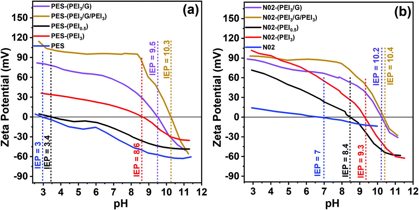 | ||
| Fig. 5 Zeta potential of unmodified PES membrane, 0.5–3 mg mL−1 PEI-modified PES membrane, graphene–polymer/PES composite membranes (a). Zeta potential of unmodified nylon membrane, 0.5–3 mg mL−1 PEI-modified nylon membrane, graphene–polymer/nylon composite membranes (b). | ||
However, it is apparent that after introducing the first PEI layer onto the support membranes, the surface charge properties change immediately and the IEP shifts to higher pH values according to the PEI concentration. A higher PEI concentration results in a bigger change in the IEP. After the first modification with 3 mg mL−1 of PEI, the IEP shifts from 3 to 8.6 for PES and from 7 to 9.3 for nylon. Additionally, it can be seen from the results that coating with graphene led to a further increase in both the absolute zeta potential values and IEP (from 8.6 to 10.3 for PES, from 9.3 to 10.4 for nylon) for both PES and nylon support membranes. Based on the electrical double layer theory60 a decrease in absolute zeta potential values can be explained by the compression of the electrical double layer due to an increase in ionic strength. The extension of the electrical double layer causes an increase in absolute zeta potential values. A further increase in the IEP occurs after the second modification of PEI, 10.3 for PES and 10.4 for nylon cases. At low pH, the surface charge of the membrane is positive owing to the existence of an abundant amino group in PEI.61 In conclusion, upon introducing PEI, the surface charge of membranes becomes more positive. It is notable that filtration and FO experiments are carried out at pH ∼ 8. Under these conditions, zeta potential of the composite membranes is around at +95 mV (Fig. 5a, yellow line) and at +81 mV (Fig. 5b, yellow line), which is beneficial for rejecting positively charged ions.
XRD patterns of graphene–polymer composite membranes fabricated using dispersion E1 (Fig. 6a and b) and E2 (Fig. 6c and d) are shown. The characteristic diffraction signal (2θ) of graphene is located in the range 26°–27°. From these results, it can be concluded that increasing the graphene loading from 0.06 to 0.16 mg cm−2 does not influence the d-spacing substantially. However, the results indicate that the average d-spacing of stacked layers is influenced by functionalization. For example, d-spacing in dry state (3.34 Å) increases slightly (3.354 Å) (Fig. 6c and d) after introducing cross-linker EDA to graphene. The peaks in Fig. 6a and b are sharper and narrower due to the presence of poorly-exfoliated graphite-like structures in the dispersion (E1) compared to the peaks in Fig. 6c and d. This is consistent with flake lateral size and thickness results obtained in graphene dispersion characterization (see Table 3). Graphene dispersions E1 have a broader thickness distribution, including thicker flakes, compared to E2. Membranes fabricated using E1 show larger crystallite size, i.e. 22 nm and 35 nm, rather than those fabricated using E2 which provide crystallite sizes of 13 nm in dry and wet states. This is also confirmed by other characterizations, which reveal that E1 contains relatively larger flakes compared to E2 (see Table 3).
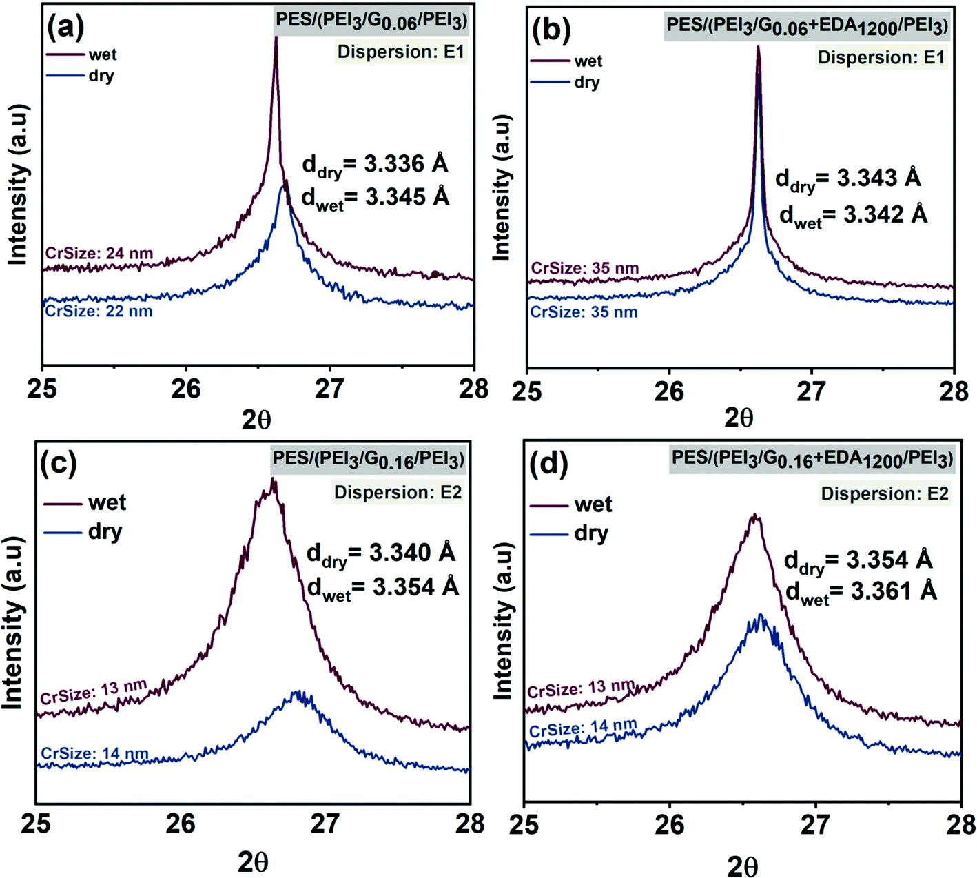 | ||
| Fig. 6 XRD analysis of graphene–polymer/PES composite membranes, without cross-linker, fabricated via dispersion E1 (a) and E2 (c) in both dry and wet phases; graphene–polymer/PES composite membranes with cross-linker fabricated via dispersion E1 (b) and E2 (d) in both dry and wet phases. | ||
Other variations of d-spacing in graphene membranes can be explained by the water which diffuses in between the graphene layers. This disrupts hydrogen bonds and π–π interactions, consequently expanding d-spacing.62 In the case of PES–(PEI3/G0.06/PEI3) and PES–(PEI3/G0.06 + EDA1200/PEI3) fabricated using E1 as shown in Fig. 6a and b, d-spacings are 3.336 Å and 3.343 Å in dry state and 3.345 Å and 3.343 Å in the wet state, respectively. In the case of PES–(PEI3/G0.16/PEI3) and PES–(PEI3/G0.16 + EDA1200/PEI3) fabricated using E2 (cf.Fig. 6c and d), d-spacings are 3.34 Å and 3.354 Å in the dry state and increase up to 3.354 Å and 3.361 Å in the wet state, respectively. The smaller changes for membranes prepared using EDA indicate that the stability of the membranes in the aqueous phase is enhanced by the cross-linked graphene. Overall, due to dominance of multi-layer graphene in the membrane, very little change in the average interlayer distance as a function of preparation route or dry vs. wet state is observed.
In conclusion, XRD data revealed that the interplane spacing essentially corresponds to the layer spacing which is found in graphite. This situation indicates the degree of exfoliation is limited. This is the reason that the content of oxygen is small because that would be only located on the surface of graphitic flakes. Hence, what is assembled on the membranes are layers of graphitic flakes (cf. Section 3.1). However, on the surface of the flakes the interactions with PEI or tartrate can take place via polar groups such carboxylate or hydroxyl, as part of the “defect” structure of the flakes (cf. Section 3.2). This is the basis for the formation of the graphene–polymer hybrid structure; with surface properties that are influenced by both components, the graphene and the polyethyleneimine (cf.Fig. 1). Additionally, it is worthy to mention that the XRD pattern of crosslinked graphene as shown in Fig. 6b is narrower compared to pristine graphene in Fig. 6a. This situation corresponds to narrower 2θ peak which demonstrates more aligned stacking while wider 2θ peak suggests a decreasing degree of in-plane orientation.63
The reaction between graphene, PEI, EDA and support membranes is further studied by FTIR spectroscopy (see ESI†). Fig. S8 (ESI†) shows the FTIR spectra of PES and nylon membranes after each assembling stage with various concentrations of PEI and graphene with or without cross-linker. However, due to the low fraction of carboxylic groups presents in the graphene, no reasonable change can be seen. This lack of distinct changes can be attributed to the limited sensitivity of IR spectroscopy.
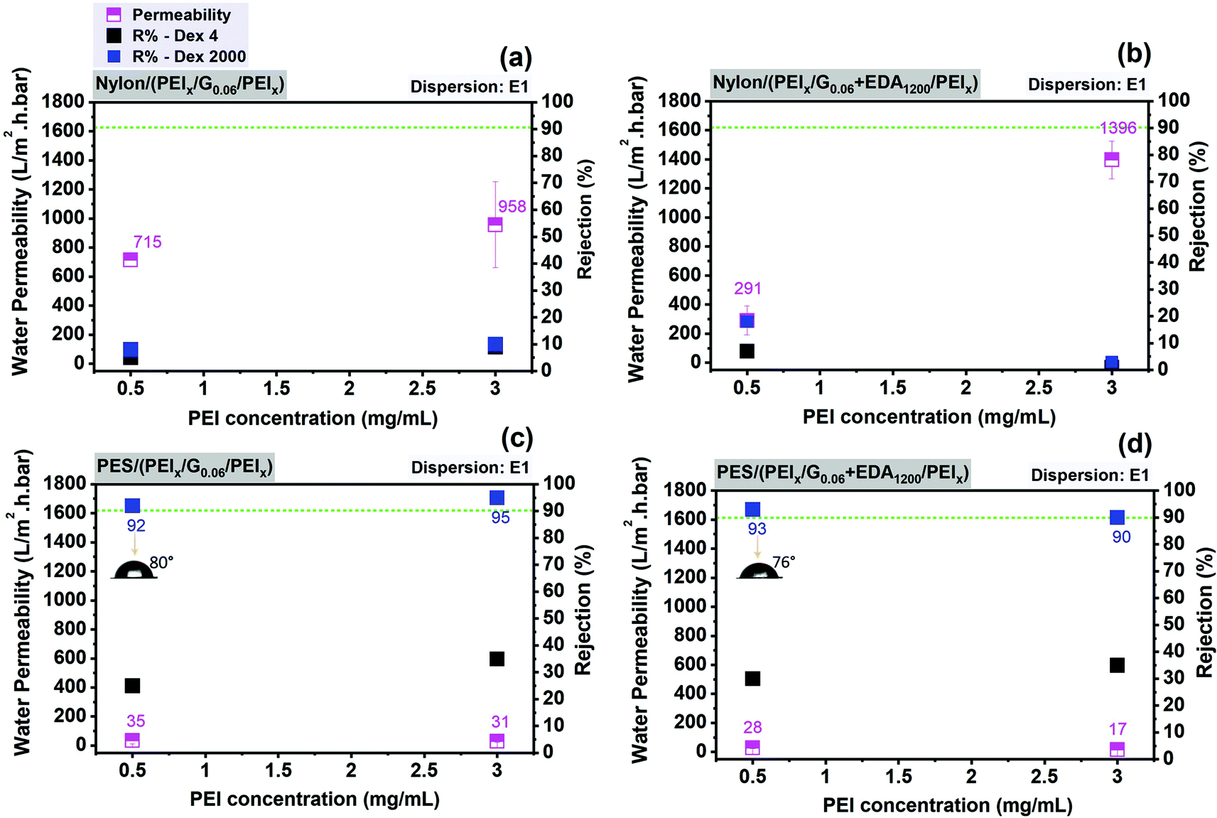 | ||
| Fig. 7 Average water permeability and dextran rejection of graphene–polymer/nylon composite membranes without crosslinked (a), with crosslinked (b) as a function of PEI concentration (mg mL−1) and graphene–polymer/PES composite membranes without crosslinked (c), with crosslinked (d) as a function of PEI concentration (mg mL−1). All membranes were prepared by dispersion E1. Contact angle measurements of the composite membranes are shown in the insets (c and d). | ||
As shown in Fig. 7c, increasing the PEI concentration from 0.5 to 3 mg mL−1 in graphene–polymer/PES membranes without cross-linker leads to a slight decrease in water permeability by a factor of 0.9. On the other hand, cross-linked graphene–polymer composite membranes (Fig. 7d) under identical preparation conditions provide a reduction in permeability from 28 to 17 L m−2 h−1 bar−1, i.e. by a factor of 0.6. Increasing PEI concentration from 0.5 to 3 mg mL−1 causes more PEI molecular chains deposition on the membrane surface. This leads to adsorption of more graphene nanosheets. In addition to decreased permeability, the rejection of dextran 2000 kDa increases by a factor of 0.96 (Fig. 7c and d) since the density of defects is decreased gradually after introducing 3 mg mL−1 PEI. In contrast, graphene–polymer/nylon composite membranes (Fig. 7a and b) provide much higher permeability in the range of 291–1996 L m−2 h−1 bar−1 compared to graphene–polymer/PES composite membranes and much lower dextran rejection, less than 20% in all cases. This might be explained by either the existence of excessively large pores in the support which are not completely covered with graphene, or major defects which contribute to the permeability and selectivity of the membranes. This was further analysed by electron microscopy. The morphology of unmodified (nylon and PES) and graphene–polymer composite coated support membranes is examined by SEM. Both support membranes have sponge-like structures, as can be seen in SEM cross-section images in Fig. 8. Furthermore, the surface of the PES membrane is smoother than the nylon membrane, as nylon has much bigger pores and irregularities on its surface (Fig. 8, top left image). Surface modification with PEI polymer does not contribute much to form a smooth surface in the nylon support case, the membranes still provide rough morphological images. This yields the creation of non-ordered graphene laminates, with high defect densities, possible in the case of nylon, which may explain the relatively poor filtration performance (cf.Fig. 7(a and b)).
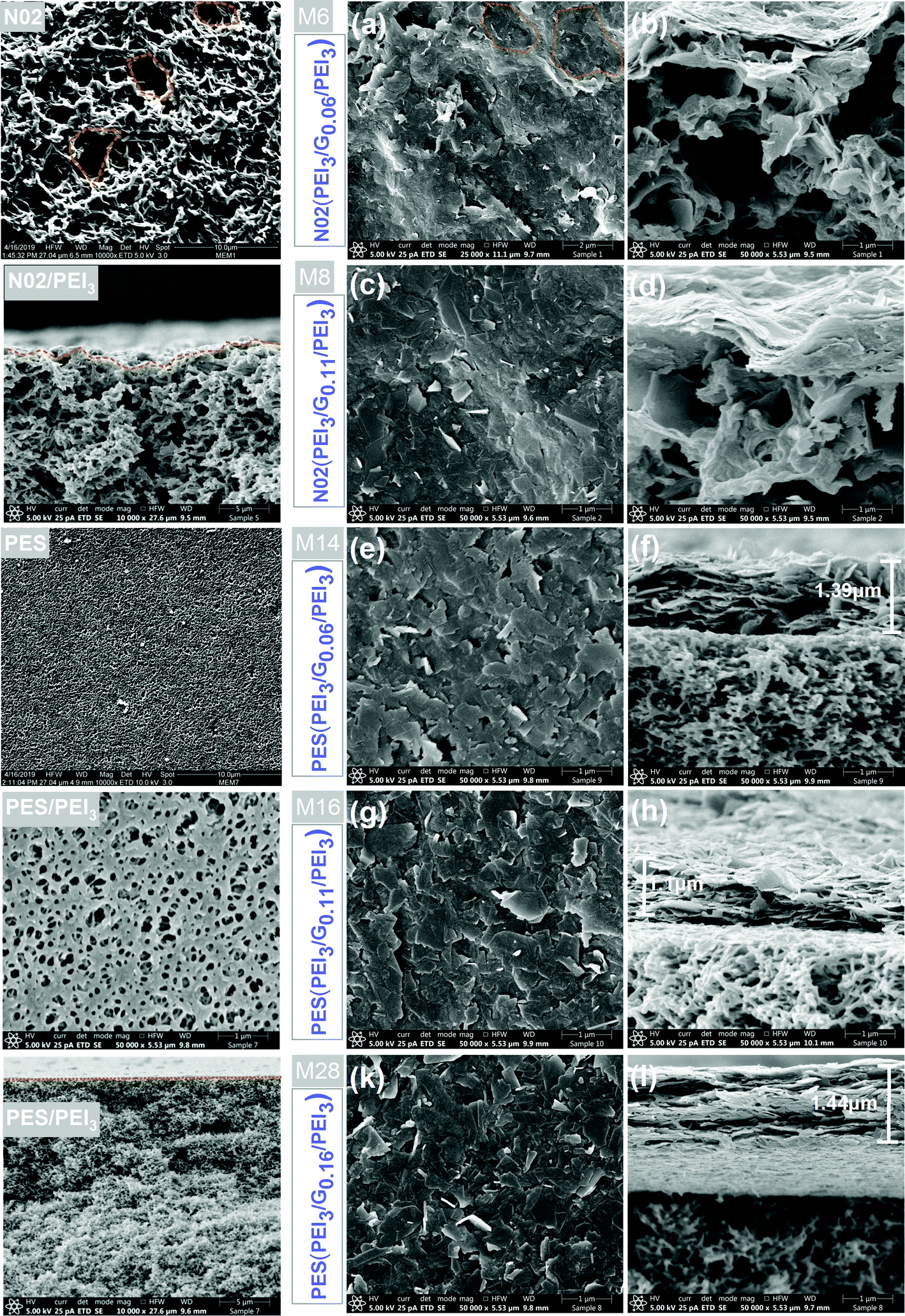 | ||
| Fig. 8 Plane-view and cross-section images of unmodified and PEI modified support membranes; nylon and PES (first left column); plane-view images of composite membranes on nylon (a and c), PES (e, g and k); cross-section images of composite membranes on nylon (b and d), PES (f, h and l). Composite membranes on nylon and PES support were fabricated by N3 and E2, respectively. | ||
As clearly shown in Fig. 8, in the case of the PES/PEI3 membrane, a higher PEI concentration causes the formation of a woven mesh-like structure of PEI on the membrane support, which is adequate for absorbing graphene nanosheets and also providing a smooth surface for graphene coating. The thickness of the selective layer of the composite membranes was measured (Fig. 8(f, h and l)). It should be noted that thickness does not increase linearly with graphene loading for both support membranes. A loosely packed graphene layer is obtained with a graphene loading of 0.06 mg cm−2. On the other hand, increasing the graphene loading up to 0.16 mg cm−2 results in a tight graphene layer, as can be seen in Fig. 8l. The type of support membrane and solvents; NMP for nylon and ethanol for PES; are the determining factors; of the selective layer thickness. For instance, 0.06 mg cm−2 and 0.11 mg cm−2 of graphene forms a layer thickness of 0.7 μm and 0.78 μm on nylon (Fig. 8b and d) while 1.44 μm and 1.10 μm on PES support membranes, respectively (Fig. 8l and h). This could be attributed to the membranes’ surface smoothness.
These results reveal that a support membrane with an average barrier pore size of 120 nm, the PES support membrane, provides better filtration performance after the assembly of graphene modified with polymer compared to nylon porous support (average barrier pore size 270 nm). In further analyses, some series of improvements are considered and studied in order to increase the quality of the graphene-based composite membranes. One focus was using a better dispersion, i.e. E2 compared to E1, in terms of the distribution of flakes size and thickness. The second decision was focusing only on the PES support membrane to obtain high-quality and high-performance graphene-based composite membranes.
In Fig. 9, various deposited amounts of graphene from dispersion E2, with and without EDA, are used in order to find the best fabrication conditions for graphene–polymer composite membranes on a PES support membrane. As shown in Fig. 9a, increasing graphene loading causes a decrease in water permeability by a factor of about 2, from 77 to 33 L m−2 h−1 bar−1 and an increase in the rejection of dextran 4 kDa up to 30% and of dextran 2000 kDa up to 94%. It is also noticeable that a further decline in water permeability, from 0.16 to 0.2 mg cm−2, is not observed. This could be attributed to the saturation point of the influence of graphene content on water permeability. In Fig. 9b, the effect of weight ratios of graphene and EDA is monitored. While keeping the graphene loading constant (0.06 mg cm−2), increasing the excess of EDA from 1:15 to 1:1500 (G:EDA ratio) causes a slight change in membrane filtration performance in terms of permeability (reduced water permeability by ∼15%, from 53 to 45 L m−2 h−1 bar−1) and rejection (increased by ∼36% for dextran 4 and ∼7% for dextran 2000). However, when keeping the EDA amount constant (1:15), increasing graphene loading from 0.06 up to 0.2 mg cm−2 causes a reduction in permeability of ∼43% (from 53 to 30 L m−2 h−1 bar−1) and a larger rise of rejection (increased by ∼75% for dextran 4 and ∼28% for dextran 2000) (Fig. 9c). These filtration results suggest that the contribution of graphene loading to membrane ultrafiltration performance is more pronounced than the amount of cross-linker. The membrane resistance is mainly affected by graphene layer. The best membranes based on the optimum filtration performance (highest water permeability with dextran 2000 rejection over 90%) obtained on the PES as support membrane and subsequently also used for FO experiments (cf. Section 3.3) have the following specifications:
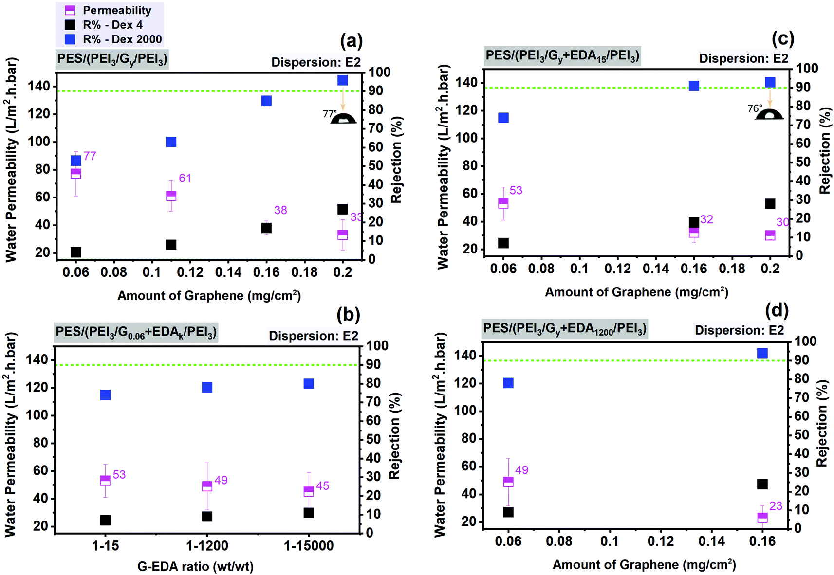 | ||
| Fig. 9 Average water permeability and dextran rejection of graphene–polymer/PES composite membranes without cross-linker (EDA) as a function of graphene amount (mg cm−2) (a), with cross-linker as a function of various graphene–EDA weight ratios (b), with cross-linker ratio of 1:15 (c) and 1:1200 (d) as a function of varied graphene loading. Contact angle measurements of the composite membranes are shown in the insets (a and c). | ||
– without using cross-linker: 3 mg mL−1 PEI for the first and third steps; 0.2 mg cm−2 graphene loading from dispersion E2; i.e. PES (PEI3/G0.2/PEI3).
It is also notable that graphene–polymer/PES composite membranes provide contact angles in the range of 70°–80°; this is still hydrophilic in nature but apparently significantly influenced by the surface properties of graphene (Fig. 7c, d and 9a, b).
Overall, ultrafiltration results suggest that a microfiltration support membrane (PES) can be successfully coated with graphene and polymer. The resultant graphene–polymer composite membranes can provide almost complete dextran 2000 kDa rejection. This is an indication that the barrier pore size of the membranes fabricated in this work is mostly smaller than 50 nm. As shown in Table 4, we can quantitatively state that the pure water permeability and rejection of our membranes are still in ultrafiltration ranges and can compete with the membranes in earlier studies.
| Membrane | Water permeability (L m−2 h−1 bar−1) | Rejection test material | R% | Ref. |
|---|---|---|---|---|
| MgSi@rGO/PAN | 4.2 | Dye (methyl orange-acid brilliant blue) | 73–98 | 66 |
| PEG-200 | 52 | |||
| PEG-1000 | 99 | |||
| rGO | 2.3 | RhB dye | 98.9 | 67 |
| g-C3N4 NT/rGO (light) | 4.8 | RhB dye | 95.6 | |
| GO–TMC/PSf | 8–28 | MB | 44–66 | 68 |
| R-WT | 93–95 | |||
| GO/PES | 27.2 | NOM | 12.5 | 69 |
| GO–EDA/PES | 10 | NOM | 34 | 69 |
| GO–PDA/PES | <20 | NOM | 24.8 | 69 |
| GO–mPDA/PES | <20 | NOM | 25.3 | 69 |
| GO/PES | 43 | HA | 85 | 70 |
| GO/PVP/PEI | 50 | HA | 77 | 71 |
| PES–(PEI3/G0.2/PEI3) | 33 | Dextran 4 | 27 | Current work |
| Dextran 2000 | 96 |
3.3. Forward osmosis characterization
The prototype membrane which provided the best ultrafiltration performance, PES–(PEI3/G0.2/PEI3; cf. Section 3.2 and Table 4) was chosen for FO experiments. The two orientations, i.e. AL-FS and AL-DS, were studied. Different types of PAA-Na with different nominal molecular weight were used, at the same nominal molar concentration (calculated with nominal molecular weight). According to the FO results (Fig. 10a), the average water flux (Jw) increases with increasing molecular weight of PAA-Na. Meanwhile, however, reverse solute flux (Js) from the draw side to the feed side also increases.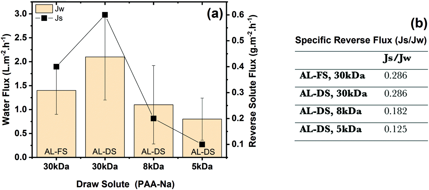 | ||
| Fig. 10 Average water flux and reverse solute flux as a function of nominal 2 mM PAA-Na 5 kDa, 8 kDa and 30 kDa measured under cross-flow conditions (a) and specific reverse solute flux (Js/Jw) (b); the mass-based concentration of the draw solutes was: 0.01 g mL−1, 0.016 g mL−1 and 0.06 g mL−1, respectively. | ||
Using water as a feed in AL-DS mode creates external concentration polarization (ECP, dilutive) in the boundary layer next to the active layer. In the AL-FS mode, “dilutive” internal concentration polarization (ICP) and concentrative ECP occur in the porous support layer and in the boundary layer next to the active layer, respectively.72 Obtained results clearly reveal that the water flux is higher in AL-DS mode (2.1 ± 0.9 L m−2 h−1) compared to that in AL-FS mode (1.4 ± 0.5 L m−2 h−1). This can be attributed to the fact that internal concentration polarization occurs in AL-FS mode, which has a greater influence on the flux decline than the external concentration polarization that mainly occurs in AL-DS mode.73
Looking at the results in AL-DS mode in more detail, water flux and reverse solute flux show an unexpected trend as a function of increasing molecular weight from 5 to 30 kDa at the same molar mass concentration corresponding to different mass concentration. At the same osmotic pressure, governed by the molar concentration, the water flux should be the same. The reverse solute flux will also depend on the diffusion coefficient of the draw solute and the barrier pore size distribution of the membrane; according to both arguments reverse solute flux should be larger for lower molecular weight.
Hence, the interpretation of the FO results is possible based on the realistic approximation of about the same molecular weight of the three different drawing agents: both water flux and reverse solute flux are a function of the different molar concentrations used (unintentionally); the highest values for Jw and Js are obtained for 30 kDa used at highest actual molar concentration and the values for 8 kDa and 5 kDa are correspondingly lower. The high specific reverse solute flux, defined as the ratio of reverse solute flux (Js) to water flux (Jw), can be explained by the fact that barrier pore size is significantly larger than the molecular size of the drawing agent. Fig. 10b reveals that the specific reverse solute flux is independent of membrane orientation. Otherwise, the apparent effect of nominal molecular weight is in reality just the effect of different actual concentrations used.
If we consider the average molecular weight of PAA-Na (30 kDa) as 1.5 kDa according to the GPC results (Fig. S9, ESI†), and re-calculate the molar concentration accordingly, the actual molar concentration would be 40 mM. As a comparison between the FO result from this work and the one from literature (Table 5), it is obvious that there is an influence between draw solution concentrations and water fluxes where low water fluxes (2.1 L m−2 h−1) are caused by a lower driving force (40 mM) compared to the one in literature (21 L m−2 h−1, 600 mM). So, FO water flux of the current membrane is comparable with a commercial one as can be seen in Table 5. However, the draw solute leakage is much higher and this is for a slightly higher molecular weight (bigger molecule size) and, more importantly, a much lower driving force for solute diffusion (because of lower draw concentration).
| Membrane | Water flux, Jv (L m−2 h−1) | Draw solution | Reverse solute flux (g m−2 h−1) | Mode | J s/Jv (g L−1) | Ref. |
|---|---|---|---|---|---|---|
| Hollow fiber CA | 21 | 0.72 g ml−1; PAA-Na (Mw: 1.2 kDa); 600 mM | 0.17 | AL-DS | 0.008 | 69 |
| PES (PEI3/G0.2/PEI3) | 2.1 | 0.06 g ml−1; PAA-Na (Mw: 1.5 kDa); 40 mM | 0.6 | AL-DS | 0.286 | Current work |
4. Conclusions
The aim of this study was to investigate using graphene, produced by liquid-phase exfoliation, for the fabrication of graphene-based composite membranes, which have desired characteristics for forward osmosis applications. The production of multi-layer graphene in organic solvents has been systematically demonstrated with the majority of flakes having lateral sizes less than 500 nm. Overall, exfoliated graphene has been successfully prepared in high or low boiling point solvents, NMP or ethanol, respectively, which provides an alternative for different purposes.Due to the better compatibility with the utilized porous polymer base membranes, ethanol-based dispersions were investigated for fabrication of composite membranes. Notable improvements have been achieved through the combination of a small but optimal amount of graphene in combination with the cationic polymer PEI on a microfiltration support membranes. Comparing the two membranes, PES and nylon, nylon provided slightly higher water permeance but poor size selectivity. In conclusion, positively charged, relatively hydrophilic graphene–polymer/PES composite membranes have been fabricated via a pressure-assisted filtration technique and systematic variations of fabrication parameter were used to maximize their filtration performance. A highly compact graphene layer sandwiched by two PEI layers provided a selective barrier with a thickness of ∼1 μm. Importantly, the composite membrane maintained its stability during filtration operation at room temperature. The overall results of this study suggest that the graphene–polymer composite membranes could be suited to achieve high water flux and sufficient rejection of macromolecular draw agents in osmotic processes.
In the current work, FO results revealed that the fabricated composite membranes are not suitable for use as a FO membrane with sufficiently high selectivity for usual draw agents which have small size, i.e., inorganic salts. Thus, the use of macromolecular draw agents would be mandatory. The applicability of PAA-Na as an alternative draw solute which provides high osmotic pressure, non-toxicity and water solubility has been evaluated. The prepared membranes exhibited comparable water flux but a high reverse draw solute flux compared to literature, which is not favourable in such systems. Nevertheless, the here established stable composite membranes with a graphene–polymer hybrid layer assembled on a macro-porous membrane support have potential and can be further tuned to the needs of special membrane-enabled separation processes.
Conflicts of interest
There are no conflicts to declare.Acknowledgements
We acknowledge financial support from Trinity College Dublin – Physics Department, German Academic Exchange Service (DAAD) and Duisburg-Essen University – Technical Chemistry II Department.References
- R. M. N. M. Rathnayake, T. T. Duignan, D. J. Searles and X. S. Zhao, Phys. Chem. Chem. Phys., 2021, 23, 3063–3070 RSC.
- A. G. Olabi, M. A. Abdelkareem, T. Wilberforce and E. T. Sayed, Renewable Sustainable Energy Rev., 2021, 135, 110026 CrossRef CAS.
- R. D. Rodriguez, A. Khalelov, P. S. Postnikov, A. Lipovka, E. Dorozhko, I. Amin, G. V. Murastov, J.-J. Chen, W. Sheng and M. E. Trusova, Mater. Horiz., 2020, 7, 1030–1041 RSC.
- P. Arpaçay, P. Maity, A. M. El-Zohry, A. Meindl, S. Akca, S. Plunkett, M. O. Senge, W. J. Blau and O. F. Mohammed, J. Phys. Chem. C, 2019, 123, 14283–14291 CrossRef.
- A. Alammar, S.-H. Park, C. J. Williams, B. Derby and G. Szekely, J. Membr. Sci., 2020, 603, 118007 CrossRef CAS.
- L. Nie, C. Y. Chuah, T. H. Bae and J. M. Lee, Adv. Funct. Mater., 2021, 31, 2006949 CrossRef CAS.
- Y. Zhang, J. Guo, G. Han, Y. Bai, Q. Ge, J. Ma, C. H. Lau and L. Shao, Sci. Adv., 2021, 7, eabe8706 CrossRef CAS PubMed.
- A. K. Geim and K. S. Novoselov, Nanoscience and technology: a collection of reviews from nature journals, World Scientific, 2010, pp. 11–19 Search PubMed.
- B. Mi, Science, 2014, 343, 740–742 CrossRef CAS PubMed.
- G. Liu, W. Jin and N. Xu, Chem. Soc. Rev., 2015, 44, 5016–5030 RSC.
- S. P. Nunes, P. Z. Culfaz-Emecen, G. Z. Ramon, T. Visser, G. H. Koops, W. Jin and M. Ulbricht, J. Membr. Sci., 2020, 598, 117761 CrossRef CAS.
- S. Fallah, H. R. Mamaghani, R. Yegani, N. Hajinajaf and B. Pourabbas, Adv. Compos. Hybrid Mater., 2020, 3, 187–193 CrossRef CAS.
- S. De, P. J. King, M. Lotya, A. O'Neill, E. M. Doherty, Y. Hernandez, G. S. Duesberg and J. N. Coleman, Small, 2010, 6, 458–464 CrossRef CAS PubMed.
- A. B. Bourlinos, V. Georgakilas, R. Zboril, T. A. Steriotis and A. K. Stubos, Small, 2009, 5, 1841–1845 CrossRef CAS PubMed.
- L. Guardia, M. Fernández-Merino, J. Paredes, P. Solis-Fernandez, S. Villar-Rodil, A. Martinez-Alonso and J. Tascón, Carbon, 2011, 49, 1653–1662 CrossRef CAS.
- A. Ganguly, S. Sharma, P. Papakonstantinou and J. Hamilton, J. Phys. Chem. C, 2011, 115, 17009–17019 CrossRef CAS.
- U. Khan, A. O’Neill, H. Porwal, P. May, K. Nawaz and J. N. Coleman, Carbon, 2012, 50, 470–475 CrossRef CAS.
- Y. Hernandez, V. Nicolosi, M. Lotya, F. M. Blighe, Z. Sun, S. De, I. T. McGovern, B. Holland, M. Byrne, Y. K. Gun'Ko, J. J. Boland, P. Niraj, G. Duesberg, S. Krishnamurthy, R. Goodhue, J. Hutchison, V. Scardaci, A. C. Ferrari and J. N. Coleman, Nat. Nanotechnol., 2008, 3, 563–568 CrossRef CAS PubMed.
- C. Backes, T. M. Higgins, A. Kelly, C. Boland, A. Harvey, D. Hanlon and J. N. Coleman, Chem. Mater., 2017, 29, 243–255 CrossRef CAS.
- M. Belmares, M. Blanco, W. Goddard Iii, R. Ross, G. Caldwell, S. H. Chou, J. Pham, P. Olofson and C. Thomas, J. Comput. Chem., 2004, 25, 1814–1826 CrossRef CAS PubMed.
- C. M. Hansen, Ind. Eng. Chem. Prod. Res. Dev., 1969, 8, 2–11 CrossRef CAS.
- A. Ciesielski and P. Samorì, Chem. Soc. Rev., 2014, 43, 381–398 RSC.
- B. Hou, H. Liu, S. Qi, Y. Zhu, B. Zhou, X. Jiang and L. Zhu, J. Colloid Interface Sci., 2018, 510, 103–110 CrossRef CAS PubMed.
- J. S. Y. Chia, M. T. T. Tan, P. S. Khiew, J. K. Chin, H. Lee, D. C. S. Bien and C. W. Siong, Chem. Eng. J., 2014, 249, 270–278 CrossRef CAS.
- A. O’Neill, U. Khan, P. N. Nirmalraj, J. Boland and J. N. Coleman, J. Phys. Chem. C, 2011, 115, 5422–5428 CrossRef.
- R. Nair, H. Wu, P. Jayaram, I. Grigorieva and A. Geim, Science, 2012, 335, 442–444 CrossRef CAS PubMed.
- Y. Han, Z. Xu and C. Gao, Adv. Funct. Mater., 2013, 23, 3693–3700 CrossRef CAS.
- F. Zhou, M. Fathizadeh and M. Yu, Annu. Rev. Chem. Biomol. Eng., 2018, 9, 17–39 CrossRef CAS PubMed.
- P. Su, F. Wang, Z. Li, C. Y. Tang and W. Li, J. Mater. Chem. A, 2020, 8, 15319–15340 RSC.
- T. Y. Cath, A. E. Childress and M. Elimelech, J. Membr. Sci., 2006, 281, 70–87 CrossRef CAS.
- W. Suwaileh, N. Pathak, H. Shon and N. Hilal, Desalination, 2020, 485, 114455 CrossRef CAS.
- S. Yadav, H. Saleem, I. Ibrar, O. Naji, A. A. Hawari, A. A. Alanezi, S. J. Zaidi, A. Altaee and J. Zhou, Desalination, 2020, 482, 114375 CrossRef CAS.
- T.-S. Chung, S. Zhang, K. Y. Wang, J. Su and M. M. Ling, Desalination, 2012, 287, 78–81 CrossRef CAS.
- Y. Cai and X. M. Hu, Desalination, 2016, 391, 16–29 CrossRef CAS.
- K. S. Bowden, A. Achilli and A. E. Childress, Bioresour. Technol., 2012, 122, 207–216 CrossRef CAS PubMed.
- S. K. Yen, F. Mehnas Haja, N. M. Su, K. Y. Wang and T.-S. Chung, J. Membr. Sci., 2010, 364, 242–252 CrossRef CAS.
- Y. Yang, M. Chen, S. Zou, X. Yang, T. E. Long and Z. He, Desalination, 2017, 422, 134–141 CrossRef CAS.
- P. Zhao, B. Gao, S. Xu, J. Kong, D. Ma, H. K. Shon, Q. Yue and P. Liu, Chem. Eng. J., 2015, 264, 32–38 CrossRef CAS.
- Q. Ge, J. Su, G. L. Amy and T.-S. Chung, Water Res., 2012, 46, 1318–1326 CrossRef CAS PubMed.
- D. Li, M. B. Müller, S. Gilje, R. B. Kaner and G. G. Wallace, Nat. Nanotechnol., 2008, 3, 101–105 CrossRef CAS PubMed.
- M. M. Devi, S. R. Sahu, P. Mukherjee, P. Sen and K. Biswas, RSC Adv., 2015, 5, 62284–62289 RSC.
- J. I. Paredes, S. Villar-Rodil, A. Martínez-Alonso and J. M. D. Tascón, Langmuir, 2008, 24, 10560–10564 CrossRef CAS PubMed.
- Y. Liang, D. Wu, X. Feng and K. Müllen, Adv. Mater., 2009, 21, 1679–1683 CrossRef CAS.
- T. Eberlein, U. Bangert, R. Nair, R. Jones, M. Gass, A. Bleloch, K. Novoselov, A. Geim and P. Briddon, Phys. Rev. B: Condens. Matter Mater. Phys., 2008, 77, 233406 CrossRef.
- Q. Lai, S. Zhu, X. Luo, M. Zou and S. Huang, AIP Adv., 2012, 2, 032146 CrossRef.
- U. Khan, A. O'Neill, M. Lotya, S. De and J. N. Coleman, Small, 2010, 6, 864–871 CrossRef CAS PubMed.
- U. Khan, H. Porwal, A. O’Neill, K. Nawaz, P. May and J. N. Coleman, Langmuir, 2011, 27, 9077–9082 CrossRef CAS PubMed.
- A. C. Ferrari, J. C. Meyer, V. Scardaci, C. Casiraghi, M. Lazzeri, F. Mauri, S. Piscanec, D. Jiang, K. S. Novoselov, S. Roth and A. K. Geim, Phys. Rev. Lett., 2006, 97, 187401 CrossRef CAS PubMed.
- Y. Hao, Y. Wang, L. Wang, Z. Ni, Z. Wang, R. Wang, C. K. Koo, Z. Shen and J. T. Thong, Small, 2010, 6, 195–200 CrossRef CAS PubMed.
- S. Karamat, S. Sonuşen, Ü. Çelik, Y. Uysallı, E. Özgönül and A. Oral, Progr. Nat. Sci.: Mater. Int., 2015, 25, 291–299 CrossRef CAS.
- D. Graf, F. Molitor, K. Ensslin, C. Stampfer, A. Jungen, C. Hierold and L. Wirtz, Nano Lett., 2007, 7, 238–242 CrossRef CAS PubMed.
- D. S. Lee, C. Riedl, B. Krauss, K. von Klitzing, U. Starke and J. H. Smet, Nano Lett., 2008, 8, 4320–4325 CrossRef CAS PubMed.
- M. V. Bracamonte, G. I. Lacconi, S. E. Urreta and L. E. F. Foa Torres, J. Phys. Chem. C, 2014, 118, 15455–15459 CrossRef CAS.
- F. T. Johra, J.-W. Lee and W.-G. Jung, J. Ind. Eng. Chem., 2014, 20, 2883–2887 CrossRef CAS.
- K. B. Ricardo, A. Sendecki and H. Liu, Chem. Commun., 2014, 50, 2751–2754 RSC.
- U. Khan, A. O'Neill, M. Lotya, S. De and J. N. Coleman, Small, 2010, 6, 864–871 CrossRef CAS PubMed.
- R. J. Smith, P. J. King, C. Wirtz, G. S. Duesberg and J. N. Coleman, Chem. Phys. Lett., 2012, 531, 169–172 CrossRef CAS.
- Y. Arao, J. D. Tanks, M. Kubouchi, A. Ito, A. Hosoi and H. Kawada, Carbon, 2019, 142, 261–268 CrossRef CAS.
- L. Yang, F. Zhao, Y. Zhao, Y. Sun, G. Yang, L. Tong and J. Zhang, Carbon, 2018, 138, 390–396 CrossRef CAS.
- D. C. Grahame, Chem. Rev., 1947, 41, 441–501 CrossRef CAS PubMed.
- Q. Nan, P. Li and B. Cao, Appl. Surf. Sci., 2016, 387, 521–528 CrossRef CAS.
- W.-S. Hung, C.-H. Tsou, M. De Guzman, Q.-F. An, Y.-L. Liu, Y.-M. Zhang, C.-C. Hu, K.-R. Lee and J.-Y. Lai, Chem. Mater., 2014, 26, 2983–2990 CrossRef CAS.
- J. Guo, H. Bao, Y. Zhang, X. Shen, J.-K. Kim, J. Ma and L. Shao, J. Membr. Sci., 2021, 619, 118791 CrossRef CAS.
- D. Venturoli and B. Rippe, Am. J. Physiol.: Renal Physiol., 2005, 288, F605–F613 CrossRef CAS PubMed.
- J. D. Oliver, S. Anderson, J. L. Troy, B. M. Brenner and W. H. Deen, J. Am. Soc. Nephrol., 1992, 3(2), 214–228 CrossRef CAS PubMed.
- B. Liang, P. Zhang, J. Wang, J. Qu, L. Wang, X. Wang, C. Guan and K. Pan, Carbon, 2016, 103, 94–100 CrossRef CAS.
- Y. Wei, Y. Zhu and Y. Jiang, Chem. Eng. J., 2019, 356, 915–925 CrossRef CAS.
- M. Hu and B. Mi, Environ. Sci. Technol., 2013, 47, 3715–3723 CrossRef CAS PubMed.
- S. Xia, M. Ni, T. Zhu, Y. Zhao and N. Li, Desalination, 2015, 371, 78–87 CrossRef CAS.
- K. H. Chu, Y. Huang, M. Yu, J. Heo, J. R. Flora, A. Jang, M. Jang, C. Jung, C. M. Park and D.-H. Kim, Sep. Purif. Technol., 2017, 181, 139–147 CrossRef CAS.
- N. J. Kaleekkal, A. Thanigaivelan, D. Rana and D. Mohan, Mater. Chem. Phys., 2017, 186, 146–158 CrossRef CAS.
- J. R. McCutcheon and M. Elimelech, J. Membr. Sci., 2006, 284, 237–247 CrossRef CAS.
- G. Gwak, B. Jung, S. Han and S. Hong, Water Res., 2015, 80, 294–305 CrossRef CAS PubMed.
Footnote |
| † Electronic supplementary information (ESI) available. See DOI: 10.1039/d1ma00424g |
| This journal is © The Royal Society of Chemistry 2021 |