
 Open Access Article
 This Open Access Article is licensed under a Creative Commons Attribution-Non Commercial 3.0 Unported Licence
Nanoparticles in analytical laser and plasma spectroscopy – a review of recent developments in methodology and applications
G.
Galbács
 *ab,
A.
Kéri
ab,
A.
Kohut
bc,
M.
Veres
d and
Zs.
Geretovszky
bc
*ab,
A.
Kéri
ab,
A.
Kohut
bc,
M.
Veres
d and
Zs.
Geretovszky
bc
aDepartment of Inorganic and Analytical Chemistry, University of Szeged, Dóm sq. 7, 6720 Szeged, Hungary. E-mail: galbx@chem.u-szeged.hu
bDepartment of Materials Science, Interdisciplinary Excellence Centre, University of Szeged, 6720 Szeged, Dugonics sq. 13, Hungary
cDepartment of Optics and Quantum Electronics, University of Szeged, Dóm sq. 9, 6720 Szeged, Hungary
dDepartment of Applied and Nonlinear Optics, Institute for Solid State Physics and Optics, Wigner Research Centre for Physics, 1121 Konkoly-Thege M. way 29-33, Budapest, Hungary
First published on 15th July 2021
Abstract
The present review attempts to comprehensively overview the progress in the field of nanoparticle-related analytical laser and plasma spectroscopy research, focusing on the results of the past decade. The discussion involves the brief description of the motivation and principle of operation behind all existing technologies. As a novel approach, the connection between nanoparticles and laser and plasma spectroscopy is discussed in all three major areas: monitoring of nanoparticle synthesis, nanoparticle characterization, as well as plasmonic signal enhancement achieved by using nanoparticles. In each area, a detailed description of methodological developments and modern applications is provided.
 G. Galbács | Gábor Galbács is holding MSc diplomas in chemistry and physics, as well as in environmental sciences (University of Szeged, Hungary). He obtained a PhD/CSc degree from the same university in 1998 and a DSc title from the Hungarian Academy of Sciences in 2013, both in the field of analytical chemistry. His research is diverse, but focuses on fundamental studies and instrumentation/method development for laser and plasma analytical spectroscopy, mostly involving LIBS, ICP-MS and ICP-AES. He is a full professor and the head of the Department of Inorganic and Analytical Chemistry at the University of Szeged since 2014. |
 A. Kéri | Albert Kéri received his B.Sc. in Environmental Engineering (2014) and his M.Sc. in Chemistry (2016) from the University of Szeged, Hungary. The topic of his PhD thesis – that he defended in 2020 at the University of Szeged – was ICP-MS-based analytical method development for the investigation of multi-component nanoparticles. He participated in several national and European founded research and R + D projects where he developed ICP-MS and LIBS based analytical methods. Currently he is a postdoctoral researcher at the Inorganic and Analytical Chemistry Department at University of Szeged. |
 A. Kohut | Attila Kohut completed his PhD in physics at the University of Szeged, Hungary in 2018. His PhD research was centered around the fundamental investigation of spark plasmas used for nanoparticle generation. Currently, his research is focusing on the generation of bimetallic nanoparticles in electrical discharges and their applications in different fields. |
 M. Veres | Miklós Veres graduated in physics at the Uzhhorod National University (Uzhhorod, Ukraine) in 2000. He received a PhD degree from the Budapest University of Technology and Economics in 2005 and a DSc title from the Hungarian Academy of Sciences in 2021, both in the field of physics. His research focuses on optical spectroscopy including spontaneous and stimulated Raman scattering, photoluminescence, plasmonic enhancement, spectroscopic imaging and instrumentation development. He is a senior researcher and the head of the Department of Applied and Non-linear Optics at the Wigner Research Centre for Physics (Budapest, Hungary). |
 Zs. Geretovszky | Zsolt Geretovszky holds an MSc in Physics and Chemistry, and a PhD in Physics, both from the University of Szeged (USZ, Hungary). He has been a research fellow at the University College London (UK) and Lund University (Sweden) and currently holds an associate professor position at USZ, where he is the head of the Nano- and Microprocessing Laboratory. Dr Geretovszky has expertise in the generation – especially in the gas phase and laser-based synthesis – and characterization of nanoparticles/nanomaterials. He co-authored more than 60 peer-reviewed publications and led several Hungarian and international R&D projects. Currently he is supervising the work of one postdoctoral and 5 doctoral fellows. |
1. Introduction
Nanoscience has moved forward with giant leaps in the last two decades. The special optical, mechanical, magnetic and energetic properties of nanoparticles (NPs) have been widely recognized and are being exploited in an array of industrial, scientific and medical fields. Today, numerous synthesis technologies are available for the controlled production of engineered NPs, nanostructures and nanocomposites not only at the laboratory, but also at the industrial scale.1–3 The influence of nanostructured materials on the efficiency and cost of, or approaches to industrial and scientific processes is so immense that many scientists consider the most recent decades as the first ones in the “nano age”, which interweaves with the silicon era.Analytical science also benefits from the special properties of nanomaterials, as it not only uses these materials, but also contributes to or provides inspiration for the development of new ones. Among others, sample preparation and separation techniques,4,5 chemical sensing6–8 and spectroscopy9–12 are the fields of analytical science that have the most interaction with nanoscience. Instrumental analytical techniques are also crucial to the characterization of NPs,13 as well as for the monitoring of nanostructures either during controlled synthesis14,15 or when released in the environment.16 This close interaction between analytical science and nanoscience has already produced a number of scientific results, which have been overviewed in several books17–19 and review papers.9,20–23
Laser and plasma spectroscopic (LPS) techniques are presently dominating the field of analytical spectroscopy. Plasma-based spectroscopy techniques, such as inductively coupled plasma optical emission and mass spectrometry (ICP-OES and ICP-MS), microwave induced optical emission spectroscopy (MIP-OES), glow discharge optical emission and mass spectroscopy (GD-OES and GD-MS), are naturally used mainly for elemental and isotopic analysis, whereas laser sources can serve both atomic and molecular analyses, depending on the laser fluence applied and the analyte reservoir. Examples include laser-induced breakdown spectroscopy (LIBS), laser ablation (LA) sample introduction, Raman spectroscopy, laser-induced fluorescence spectroscopy (LIFS), photoacoustic spectroscopy (PAS), laser enhanced ionization spectroscopy (LEIS), cavity ringdown spectroscopy (CRDS) and more.24 More recently, the combination of laser and plasma sources for analytical spectroscopy purposes is also gaining momentum, used either as a performance booster (e.g. ref. 25 and 26), or in tandem (hyphenated) instruments in order to provide more, atomic plus molecular, analytical information about the sample. In the latter bin, often are instruments which involve LA and LIBS, for the reason that these techniques lend versatile sampling and spatial resolution capabilities to other analytical spectroscopies. LIBS-Raman,27 LIBS/LA-ICP-MS,28 LA-GD-MS29 and LIBS-LIF30 are examples for such tandem instruments.
Nanomaterials are also more and more involved with lasers and plasmas. For instance, nanoparticle synthesis by electrical discharge plasmas1,31 or via laser ablation32 are recently becoming increasingly common methodologies. Since the most popular engineered NPs are metallic therefore laser and plasma based atomic spectroscopies are most often called for the in situ monitoring of the synthesis process or for the characterization of the produced particles. LIBS33–35 and ICP-MS seem to show the best performance and practicality in these applications. In particular, the single particle ICP-MS (spICP-MS) technique has become a very powerful and versatile nanoparticle characterization approach36,37 for nanosols. Laser light scattering38 and absorption methods (such as PAS39), are also well established, important tools of nanoaerosol characterization. Analytical signal enhancement in LPS is also often effectuated by using nanoparticles, mostly based on plasmonic effects. A premier example for this is surface enhanced Raman spectroscopy (SERS),10 but LA-ICP-MS40 and LIBS12,41 applications are also benefiting from similar effects. Last, but not least, the use of NP-based liquid sample preparation methodologies in LPS in general, such as separation or preconcentration, are also becoming more frequent in recent literature.
Several reviews overviewed earlier the applications of nanomaterials in analytical science in general,9,20–23 but so far none focused on the field of laser and plasma spectroscopy, while this field enjoys a steadily increasing involvement of nanomaterials in recent years. The closest scope was provided by the review of Jiang et al.9 in 2012, which covered applications in analytical atomic spectrometry. Therefore, the present review attempts to encompass and comprehensively overview the recent developments in all main areas of laser and plasma spectroscopy which interact with inorganic nanoparticles: namely the monitoring of the synthesis of nanoparticles, the detection and characterization of nanoparticles and the use of nanoparticles for signal enhancement. Please note that the scope does not include single macromolecule analysis. Our review focuses on results that appeared in the literature in about the last decade. Brief overviews of the methodologies of included subfields will be provided, along with references to seminal books and pioneering works, but the focus is on recent applications.
2. Monitoring of nanoparticle generation
2.1. Importance, driving force and overview
NP synthesis methods range over numerous techniques, including chemical, physical, mechanical, and even biological approaches.42–44 While there are some “golden standards” of NP characterization, such as transmission electron microscopy, certain generation methods have their unique characterization toolbox which fits the conditions of the given production method best. This is especially true when the monitoring of the whole synthesis process is aimed. Laser- and plasma-based spectroscopic techniques proved useful for in situ monitoring of particle formation in a temporally and/or spatially resolved and – potentially – minimally invasive manner. Plasma spectroscopic monitoring is a natural choice when NP generation process includes a plasma stage, such as in the case of laser45 or spark46 ablation, but it can also be useful when plasma is generated from the already formed particles by means of an energetic excitation source, such as a laser pulse.47 The development of the spectroscopic toolbox used for monitoring plasma-based NP generation dates back long before the introduction of the term “nanoparticle”. Although in early research the occurrence of microscopic particulates was mostly considered as a side-effect,48 the accumulated knowledge on material removal from the target,49 on the excitation of different species,50 or on the determination of important plasma parameters51 provided valuable contribution to the plasma spectroscopic monitoring of current NP generation techniques. The application of lasers in monitoring the NP generation opens up further possibilities via selectively exciting particle populations even at different stages of their formation. Various approaches exist, depending on the laser–particle interaction initiated, such as laser-induced incandescence (LII),52 laser-induced breakdown spectroscopy (LIBS),53 elastic,54 or inelastic55 scattering, or absorption,56 to mention but a few. In the following sub-chapters, we will summarize some of the most recent laser- and plasma spectroscopy methods applied for the monitoring of NP generation, after a brief description of the plasma diagnostic methodology related to this analytical problem.2.2. A concise introduction to plasma diagnostics
Plasma diagnostics incorporates a broad variety of techniques aiming to give a comprehensive description of plasma properties. When plasmas are utilized as sources for NP synthesis, plasma diagnostic tools allow for the precise measurement of synthesis conditions, hence facilitating the better understanding of particle formation mechanisms as well as providing more control over the generation process. Plasmas are different from other, more common states of matter, first and foremost in that their most important properties are generally cannot be measured directly. Instead, plasma properties are deduced from observations of physical processes and their effects.57 This approach greatly relies on the understanding of plasma physics and chemistry involved in said processes. It rather naturally follows from the above that modeling the plasma, or at least those aspects which are subject of investigation, is often an integral part of plasma diagnostics. Since a complete description of the distribution function of the plasma constituents' position and velocity is not feasible in general, plasma diagnostics usually aims at determining the so-called lower order moments of the distribution function, such as the density, mean velocity, pressure, temperature, and heat flux. Numerous techniques exist for obtaining these values, along with multiple possibilities to categorize the different methods.One way to sort plasma diagnostic techniques is based on the physical process or property of the plasma that is measured, as proposed by Hutchinson in his very comprehensive book on plasma diagnostics.57 By following this approach magnetic, particle flux, and refractive index measurements, the measurement of photon emission from free or bound electrons, as well as the measurement of interaction with electromagnetic waves can be distinguished. Since the detailed discussion of these experimental approaches are far beyond the scope of the present review, we will only briefly overview some of the main aspects of the interpretation of the emission from free and bound electrons, i.e., the topic of plasma emission spectroscopy.
Optical plasma emission spectroscopy (OES) is a versatile tool for diagnosing laboratory plasmas, with a well-established theoretical and instrumentational background.58–60 Apart from the identification of species present in a plasma, the two main parameters that are predominantly determined by OES are the number concentration of electrons (electron density, ne) and the electron temperature (Te).61 In order to support the following sub-chapter, we will briefly mention some widely used methods for calculating ne and Te, usually employed during the monitoring of plasma-based NP synthesis.
In case of laser- and electric discharge plasmas, electron concentration is mostly calculated from the spectral broadening of emission lines, predominantly assuming that Stark broadening is the dominant mechanism.62,63 Stark broadening and line shifting results from the Coulomb interactions between the emitting species and the charge carriers present in the plasma. Due to the availability of precise tabulated data and validated theoretical description, the Stark broadening of H lines – especially the Hβ line – are widely used to determine the electron concentration in plasmas.64–66 If H atoms are not present in the plasma, other elements can also be used to estimate the electron concentration, however, in this case the accuracy is usually lower, deviations typically in the range of 15–50% can be found.65,67 Even though, various theoretical models exist to interpret Stark-broadened spectral lines,68 in most of the practical cases electron concentration is estimated based on the comparison of the broadened full width at half maximum (FWHM) or line shift with reference data,69 tabulated for various transitions.70–72 The following two equations are adapted from ref. 69. Eqn (1) describes the electron concentration as a function of the Stark-broadened FWHM for hydrogen and hydrogen-like ions:
| ne = C(ne,Te)ΔλS3/2 | (1) |
 | (2) |
It should be noted that in some cases the effect of other line broadening mechanisms (such as instrumental, Doppler, resonance, van der Waals broadening) cannot be neglected, therefore the contribution of the Stark effect to the overall line width – often called Stark width – must be determined. To this end, various deconvolution procedures can be used depending on the relative importance of the different mechanisms.73,74 In certain cases, deconvolution procedures allow for the simultaneous derivation of electron concentration from the Stark component and the electron temperature from other mechanisms, such as Doppler73 or van der Waals75 broadening. It should be mentioned that different approaches also exist for determining the electron concentration from the emission spectrum of a plasma, e.g., by using absolute irradiance methods, which usually require the calibration of the spectrometry setup and the modelling of the emission spectrum.76,77
The other important plasma parameter, which can be derived by means of plasma OES, is the electron temperature, Te. It should be noted that plasmas are generally described by several different temperature values, corresponding to different plasma constituents (such as electrons, atoms and ions) or processes (such as atomic excitation and molecular vibrations or rotations). In many cases, these temperatures are not equal, hence different approaches are needed to determine a specific temperature value. However, there are certain cases, when some sort of equilibrium can be assumed, thus making temperature determination much easier. This is the case when local thermodynamic equilibrium (LTE) prevails in the plasma. Simply speaking, LTE means that different species present in the plasma have the same local temperature.78 To reach LTE, the electron concentration needs to be sufficiently high in the plasma facilitating collisions with electrons to be dominated over radiative processes. In this case, a single “LTE temperature” can be derived, representative to the temperature of the electrons as well. Here we will briefly overview the most popular method used for estimating T from the emission spectrum of a plasma assumed to be in LTE, usually called the Boltzmann plot method. As suggested by the name, it is related to the Boltzmann equation, which describes the population of excited energy levels as a function of temperature.58 Since the emission line intensities characteristic to different transitions of an atom or ion are proportional to the number concentration of the species in the corresponding excited states, a relation can be found between the emitted line intensities (Iij) and the so-called excitation temperature governing the population of the excited states, described by the following equation:
 | (3) |
 | (4) |
It is apparent from eqn (4) that the excitation temperature, which in LTE equals to Te, can be derived from the measured line intensities and the atomic data corresponding to the relevant transitions. A minimum of two emission lines are needed to calculate the temperature by using the Boltzmann equation – often called line-pair method,79 or two-line method80,81 – but the results are generally more reliable when more spectral lines are involved, preferably with a wide spread over the upper energy level. In this case, the temperature is given by the slope of the graph described by eqn (4).51,82
As it was already noted, Boltzmann plot method relies on the assumption that local thermodynamic equilibrium (LTE) – at least partially, for the corresponding transitions – exists. The validity of LTE can be estimated based on the electron concentration from the Griem83 or McWhirter84 criteria. Even though these criteria are widely used to justify the presence of LTE in atmospheric pressure laser- and arc or spark plasmas,51,69,85 there are indications that a more thorough analysis should be made to assess the validity of the assumption of LTE.86 When deviation from LTE prevails, the Boltzmann plot method can still be employed to derive the excitation temperature by introducing correction factors.51 Nevertheless, the temperature determined from the Boltzmann plot method describes the temperature of the electrons only when the presence of LTE is justified.
Originally, the Boltzmann plot method can be applied to a single species in a given ionization level. However, by exploiting the fact that in LTE the population of different ionization stages are determined by Te and ne, one can extend the method to successive ionization stages. The method that incorporates this extension is called the Saha–Boltzmann method, named to refer to the fact that the ionization equilibrium is described by the Saha equation (eqn (5)):51,69,87
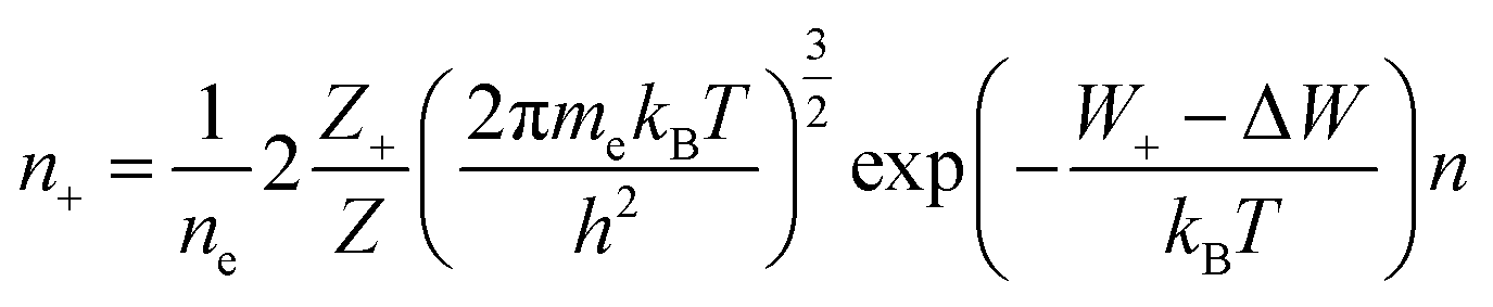 | (5) |
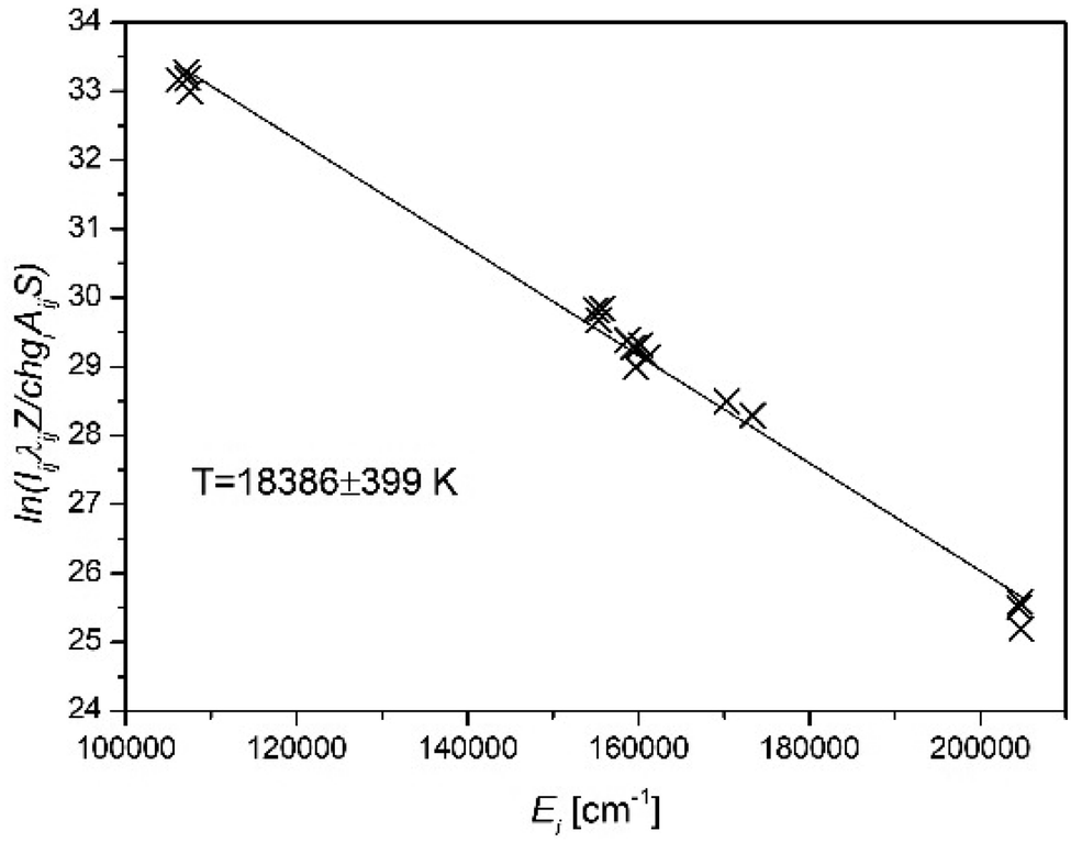 | ||
| Fig. 1 Saha–Boltzmann plot constructed from the emission spectrum of a Cu/Ar spark discharge plasma measured ca. 1 μs after the onset of the gas breakdown (based on the authors' own data). | ||
We have already mentioned the importance of LTE in Boltzmann plot methods, but there are several additional considerations which should also be kept in mind. Here we only briefly list some of these considerations, for further details please refer to the cited literature. First, it is important to note that the accuracy of constants involved in the equations highly affect the accuracy of the calculated values. The most critical factor here is the transition probability, which in many cases is only known with poor accuracy.65 It should also be noted that the above methods are applicable for optically thin plasmas. Therefore, when self-absorption is dominantly present in the emission spectra, additional techniques or corrections must be applied.69,90–92 It should also be kept in mind that OES techniques provide spatially integrated information over the line of observation. Therefore, spatial deconvolution techniques might need to be applied. For instance, a commonly used technique for optically thin plasmas with cylindrical symmetry is the Abel inversion. By employing Abel inversion, the radial intensity distribution can be reconstructed from the lateral intensity distribution.69
The above-mentioned methods rely on the line emission of the plasma for temperature determination, but additional OES-based plasma diagnostic techniques also exist. The continuum radiation emitted by plasmas – highly characteristic to the early stages of laser ablation plasmas69 – can be exploited for temperature calculation via the so-called line-to-continuum intensity ratio method. As suggested by its name, this method employs both the intensity of the spectral lines and the continuous component of the emission spectrum to derive the electron temperature under LTE conditions.93 Apart from the importance of sufficiently well-known parameters and constants, which cannot be stressed enough at all OES-based methods, the applicability of this approach is also limited to those stages of plasma evolution when line spectrum coexists with continuum radiation, both having sufficient signal-to-noise ratio.69
It should also be mentioned that LTE conditions are often not met in many plasmas, however, OES- (and laser spectroscopy) based methods are still proved useful in the description of these plasmas. An important parameter of non-LTE plasmas is the rotational temperature of molecules present in the plasma, which is often assumed to be equal to the – translational – gas temperature. There are various techniques for obtaining the rotational temperature from emission (and absorption) spectra, which were critically reviewed recently by Bruggeman et al.94 We only mention that when an equilibrium rotational population is assumed, essentially the Boltzmann plot method can be applied to the determination of the rotational temperature, with the difference that rotational spectral lines must be used for constructing the plot. Simulating the rotational spectrum and fitting to its measured counterpart is also a commonly used method for deriving the rotational temperature. This approach has the advantage that depending on the complexity of the model used for generating the synthetic spectrum, more thorough description of the analyzed plasma can be given than in case of equilibrium-based methods.
2.3. Methodology and applications
Laser- and plasma spectroscopic methods are predominantly used in the in situ monitoring of NP generation in particle synthesis techniques where the initiation of a plasma is involved, such as electrical discharges (mostly arcs and sparks), laser ablation, and flames. Therefore, in the following subchapters we will focus on the monitoring methodology applied in these synthesis methods, while some further synthesis routes where in situ laser- or plasma-based particle monitoring were utilized will be mentioned at the end of the chapter.Since optical diagnostic methods are capable of providing this information without disturbing the synthesis process, a broad range of techniques have been developed or applied to the specific conditions of flame synthesis. Fig. 2 schematically shows the particle generation in a flame reactor and exemplifies several optical and non-optical diagnostic tools for the in situ and ex situ investigation of different aspects of the particle formation process. Optical diagnostic methods applicable for monitoring flame synthesis were thoroughly reviewed very recently by Dreier and Schulz,100 Schulz et al.,101 and Rahinov et al.102 therefore we only recall here some of their main considerations supplemented by related literature.
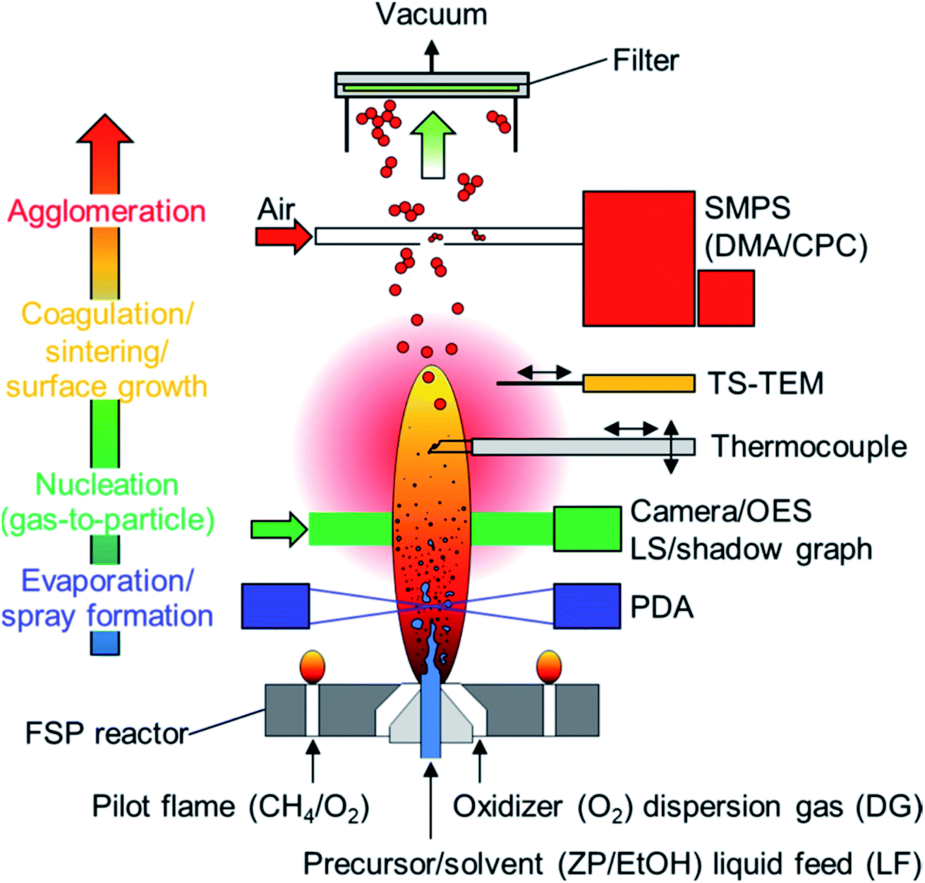 | ||
| Fig. 2 Schematic figure of an experimental flame spray pyrolysis (FSP) reactor setup and process diagnostics for analyzing the consecutive stages of metal oxide NP evolution. Nonintrusive laser and camera diagnostics including phase-Doppler anemometry (PDA), laser sheet (LS) and shadow graphic (SG) for liquid spray analysis (blue), as well as optical emission spectroscopy (OES) and camera imaging for determination of the metal oxide nanoparticle nucleation zone (green). Thermophoretic sampling with subsequent transmission electron microscope analysis (TS-TEM, orange) and scanning mobility particle sizer (SMPS, red) are applied for local description of primary and agglomerate nanoparticle evolution, while filter collected particles are considered for ex situ analysis (BET and XRD). Figure and caption are taken from ref. 99. | ||
Laser-based methods applicable for the in situ monitoring of flame NP synthesis can be divided into two main groups, the first includes the methods appropriate for monitoring the gas-phase particle formation process (such as the temperature and intermediate species concentration), while the second group consists of the techniques capable of monitoring the properties of the generated particles.100 A commonly used method both for temperature and concentration measurements is based on the absorption of a laser beam. Information on the average temperature or concentration of intermediate species (such as small molecules corresponding to precursor reactions) can be gained by measuring the absorption spectrum by using ring-dye lasers or tunable diode lasers, employing Fourier-transform infrared spectroscopy (FTIR), intra-cavity laser absorption spectroscopy (ICLAS), or cavity-ring-down absorption spectroscopy (CRDS).100 Even though absorption-based techniques provide line of sight information, by employing fan-shaped laser illumination and multiple detectors, temperature and concentration distributions can be reconstructed using a 1D tomographic algorithm.103 Another method enabling the online monitoring of the flame temperature and the concentration of the intermediate species is laser-induced fluorescence (LIF). LIF methods are usually distinguished by the species the measurements are based on, such as NO or OH for temperature, and various other species (e.g., Fe, CH2O, CH, OH, SiO, FeO, In, AlO, TiO) for intermediate concentration determination.100 Recently, the good applicability of SiO-LIF in quantitative temperature104 and concentration105 imaging as well as the investigation of the combustion chemistry of the flame synthesis of SiCl4 nanoparticles106 have been demonstrated.
In addition to the above techniques, the temperature can also be determined based on both elastic and inelastic scattering of laser light. Raman- and coherent anti-Stokes Raman scattering (CARS) as well as Rayleigh scattering have been applied to measure the temperature in flame reactors,100 however, since these techniques are more suitable for particle-free environments, usually they are of limited use in strongly particle-laden flows.101 Apart from temperature measurements, light scattering-based techniques can also be used to monitor the properties of the as formed particles in situ. For this purpose, another laser-based technique is the so-called laser-induced incandescence (LII), which is based on the measurement and analysis of the incandescence signal of the particles heated up by a laser beam, providing information on volume fraction and primary particle size100 (see Section 3.3.2. for details). Since the proper interpretation of the LII signal is not straightforward, attempts are made to standardize calibration and signal processing protocols.107,108 When the laser fluence is high enough to vaporize the NPs, the emitted atomic spectrum can also be used to gain information on the particles. This is the basis of laser-induced breakdown spectroscopy (LIBS), a technique well-known in analytical spectrochemistry109 (see Section 3.3.3. for details). In situ aerosol LIBS is relatively challenging to execute and interpret the results, but it has been shown to be able to provide valuable information on the complex processes taking place in turbulent flame reactors.110
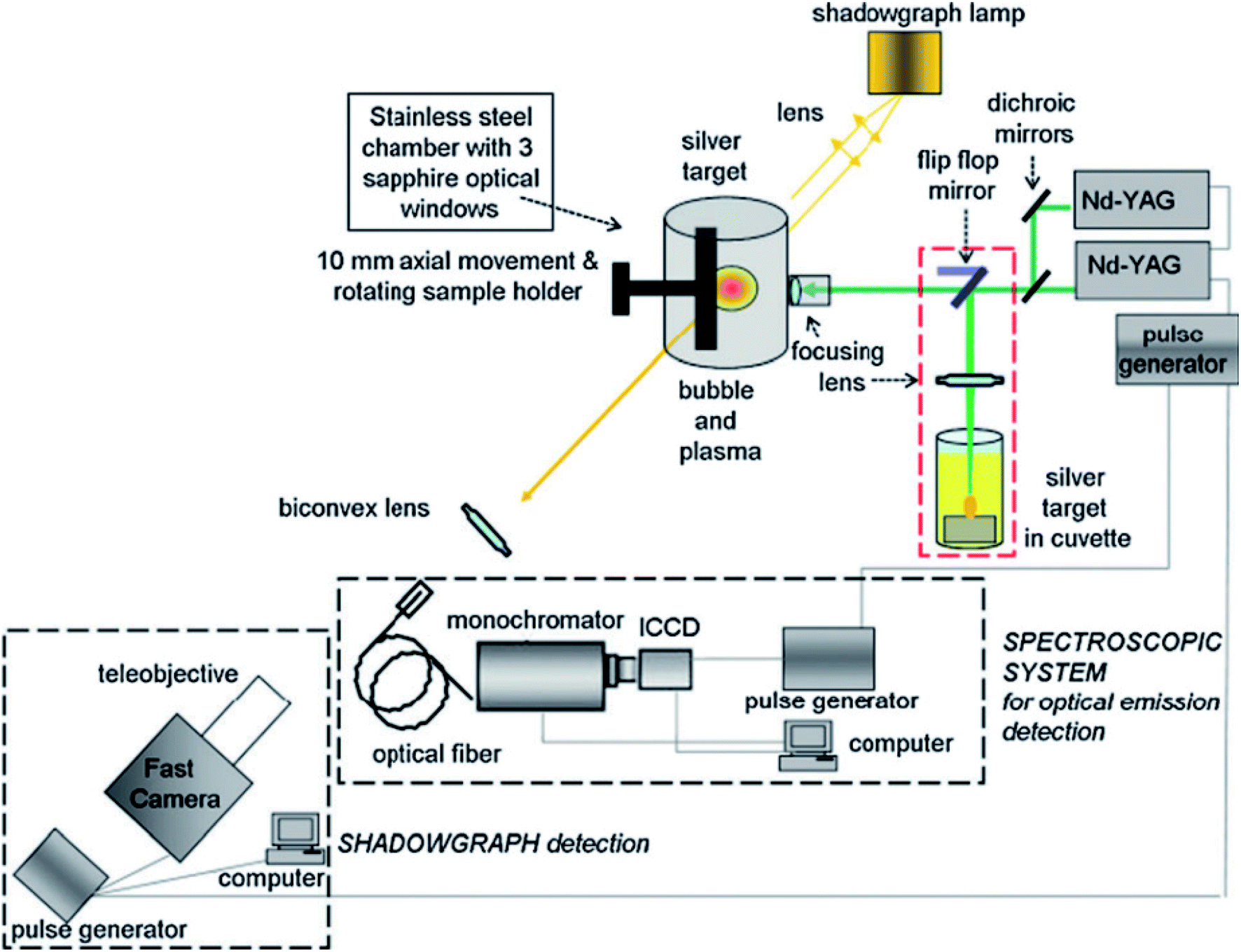
The most basic approach for the monitoring of the laser-induced plasma (LIP) is the collection of its temporally and spatially integrated radiation by means of an optical fiber during the ablation process. Thereafter, e.g., the Boltzmann plot method (see in Chapter 2.2.) can be applied to calculate the excitation temperature of the plasma,115,116 or the Stark broadening to derive the electron concentration.117 Naturally, much more reliable data can be obtained when the highly transient LIP is monitored with appropriate temporal resolution. Evolution of electron concentration as derived from Stark broadening,118–120 temperature evolution calculated from the Boltzmann plot120 and Saha–Boltzmann plot,118,121 or relative line intensity119 methods are routinely applied. It should be noted that even in case of temporally resolved measurements, care should be taken when temperature calculation methods relying on the existence of LTE are applied. This is especially true in case of low-pressure laser ablation experiments where electron concentration decreases rapidly, hence LTE can only be assumed in the earliest stages of the laser plasma.122 Another circumstance, which necessitates high temporal resolution is the limited temporal detectability of the emission signal, as in case of pulsed laser ablation under liquid (PLAL), where the signal is detectable for only a short period of time (a few tens of nanoseconds to a few microseconds). Nevertheless, by employing a high temporal resolution ICCD camera, the evolution of the plasma emission can be monitored123 and the plasma temperature can be deduced in this short interval e.g., by fitting the continuum component of the emission spectrum by a Planck-like distribution,114 or by employing the Boltzmann plot method to the spectral lines.124 A typical experimental setup for OES-based monitoring of NP generation during PLAL is shown in Fig. 3. The temperature can also be deduced by comparing the measured and simulated vibrational and rotational spectra of the plasma, supplemented by electron concentration determination from the Stark broadening of spectral lines.125
 | ||
| Fig. 3 Schematic of the experimental setup for the OES-based monitoring of NP generation by pulsed laser ablation in gas and liquid.114 | ||
Apart from the calculation of plasma parameters (such as temperature or electron concentration), the intensity variation of specific spectral lines also carries important information on the particle generation process. Such information for instance is the transfer of species dissolved in a liquid into the plasma created during PLAL. By following the intensity variation of two ionic lines the spectral features can be correlated to the composition of the ablated sample and thus the transfer process can be investigated.126 Similarly, by comparing the emission intensity of an atom to that of the ion or oxide of this atom, the dynamics of the ionization or oxidization processes can be monitored.118,125 Direct information on the variation of atomic or ionic spectral lines is also useful when spatially and temporally resolved OES is employed to monitor one or more process parameters of the laser ablation process, such as the ablation medium (e.g. gas or liquid),119 ablation wavelength121 or the ambient pressure.127–130 Having spatial, temporal, and spectral resolution at the same time allows for carrying out time-of-flight measurements of specific species generated during laser ablation. The expansion dynamics of selected plasma constituents can be derived from the emission spectra and used for instance in correlation with the excitation processes,130 or to detect the onset of the deposition process and the growth of a NP film during PLD.121,127,131,132
It should be noted that temporally and spatially resolved OES is predominantly carried out by acquiring a relatively broad spectrum of a localized spatial region with a ns-gated camera, thus obtaining information on several species at the same time. However, this indicates that an extended area can only be covered by “scanning”, i.e., repeating the measurements in different locations. In contrast, when the spatio-temporal investigation of only one or a few specific spectral lines is aimed, high spatial and temporal resolution can be achieved at once by imaging the plasma after using a wavelength-dispersive element.133 Additional information can be gained on the particle formation process by employing a second laser pulse to excite the species ablated by the main pulse. The second pulse can be either collinear114 or orthogonal124 to the main pulse, and the emission of the excited species can be used to calculate the excitation temperature via the Boltzmann plot method, or the electron concentration from Stark broadening.114 A remarkable feature of this double-pulse approach is the correlation of the emission generated by the second pulse with the changes associated with the first pulse, be it the dynamics of bubble formation under liquid,114 or the composition of the generated nanoparticles.124
In the above cited studies, optical emission of the laser-generated plasma was acquired and analyzed during NP generation to monitor the particle synthesis process. However, different approaches also exist, which use plasma- and/or laser spectroscopic techniques for the in situ characterization of the laser ablation-generated particles and therefore monitor the generation process. Dynamic light scattering (DLS) is a widely used technique to investigate NPs dispersed in a liquid,38,134 see Section 3.3.1. for details. Wei and Saitow have demonstrated that DLS can be used in connection with a pulsed laser ablation NP generation system for the in situ monitoring of particle synthesis in a supercritical fluid.135 As opposed to the seconds to hours temporal domain covered by the DLS measurements of Wei and Saitow, temporal resolution in the picosecond range can also be achieved via femtosecond transition absorption spectroscopy. By employing sub-picosecond pump and probe laser beams, the evolution of the transient absorption spectrum of gold NPs exposed to pulsed laser irradiation could be followed.136In situ probing a femtosecond laser plasma was carried out by Oujja et al. They have employed a second, nanosecond laser pulse perpendicular to the material ablating laser to generate its third harmonics and obtained its spatiotemporal distribution from nanoseconds to hundreds of microseconds after ablation. It was concluded that the harmonic generation is affected by the formation of middle-sized metal clusters that had a huge effect on the harmonic generation yield. Thus, this nonlinear optical approach is capable of investigating the cluster formation during fs-laser ablation-based NP generation.137 All the previous methods exploited the investigation of the optical response of the laser plasma or the generated NPs, induced by laser excitation. However, as demonstrated by Valverde-Alva et al., the photoacoustic signal generated during the laser ablation of a target in ethanol can also be used to monitor the NP generation process.138 Their results exemplify well that the acoustic signal generated by the ablating laser pulses is also useful for the in situ monitoring of laser ablation-based NP synthesis.
Electric sparks are not self-sustaining discharges, meaning that after the initiation of the breakdown of the medium between the electrodes, energy must be continuously supplied externally to maintain sparking.147 The way of the energy input, the design of the electrodes or the surrounding medium may vary, thus greatly influencing the discharge characteristics, including the existence or non-existence of LTE in the discharge plasma. One form of spark discharges associated with the formation of a thermal plasma is utilized in the so-called spark discharge nanoparticle generators (SDGs).148 SDGs are based on the spark ablation of a pair of electrodes placed in a gas-tight chamber under atmospheric pressure. The sparking is maintained by periodically discharging a capacitor (typically having a capacitance in the range of a few or a few tens of nF) connected to the electrodes. The sparking is associated with an energetic discharge plasma allowing for high currents (several hundreds of amperes) to flow between the electrodes typically for a few microseconds, resulting in the atomization of the electrode material. This material is quickly cooled down due to expansion and the presence of a gas stream continuously flowing through the interelectrode gap. This gas flow also carries away the ablated material and facilitates the formation of NPs.149,150 The generated NPs are dispersed in the carrier gas thus forming an aerosol. Aerosol science has well established methodologies to analyze the produced particles both in situ151–153 and ex situ.154 However, an inherent limitation of these techniques is that they only provide information about the “final product” of the process – i.e., the NPs – and therefore unable to monitor the generation process itself, especially the initial plasma stage.
Optical diagnostics of thermal spark plasmas has a long history with well-established methodology and scientific results, mostly driven by the research interest in the field of analytical spectrochemistry. Spark plasmas include transient, temporally and spatially varying phenomena the reliable investigation of which necessitates the use of temporally – and preferably spatially – resolved techniques.155 Due to the analytical perspective, the early studies in the field mostly focused on the direct analysis of the emitted light in order to understand the sampling and excitation mechanisms taking place in the spark.156 Those studies mostly included the determination of the concentration of the ions and electrons by utilizing the Stark effect,64 or laser scattering,157 or interferometry.158 Calculation of the plasma temperature by means of the Boltzmann159 or the Saha–Boltzmann plot method51 has also been carried out. A comprehensive overview of the methods applicable for gas discharges can be found in the book by Boumans,50 while the fundamental mechanisms obtained during the analysis of the spark emission is reviewed by Scheeline.49
These results serve as an important basis for the optical monitoring of electrical discharge-based NP generation; however, they cannot be directly applied for modern SDGs. The reason for this is, in contrast to the highly regulated and well-controlled analytical sparks, SDGs are mostly operated in “free running mode” when sparking occurs as soon as the breakdown voltage of the interelectrode gap is reached.160 The lack of regulating circuitry results in a technically simple and easy-to-construct design and a higher particle yield, but also hinders the use of external instrumentation with precise active triggering and sometimes poses stability issues. Other technical constraints, originating from e.g., the generator chamber or the components of the gas line also introduce physical limitations which narrows the range of applicable methods. All the above considerations rather naturally lead to the use of OES as a useful spectroscopic technique applicable under the circumstances of NP generation. In its most basic form, OES can be applied simply to analyze the emission originating from the spark gap without spatial or temporal resolution. Hontañón et al. used an optical fiber to collect the light emitted by the spark plasma during NP generation and analyzed its spectrum by a simple tabletop spectrometer. The acquired spectra reflected the spatially and temporally averaged spectrum of several concomitant sparks but still provided useful information about the conditions of the generation process. They have collected the spectra of a continuous glow and arc discharge used for NP generation as well and demonstrated that even with such an experimentally simple OES approach, the three discharge regimes are clearly discernible.161 This has great potential in the optical monitoring of electrical discharge-based NP generators.
A much deeper insight can be gained by acquiring time-resolved spectra of the spark plasma, an experimental setup for which is shown in Fig. 4. In a similar arrangement, Kohut et al. employed a fiber-coupled echelle spectrograph equipped with an intensified CCD to investigate the temporal evolution of the spectrum emitted by a spark plasma during NP generation, with the concomitant fast imaging of the sparking, with a temporal resolution of 50 ns.85 Due to the already mentioned unregulated nature of the sparking, the spectral acquisition was synchronized to the plasma formation by using the sharp drop of the capacitor voltage as a trigger signal. This introduced a ca. 100 ns time delay, which inherently means that the very first stages of a spark discharge – i.e., the so-called pre-breakdown and breakdown stages162 – cannot be investigated by this approach. These temporal periods, however, are considered to have minor contribution to NP generation, compared to the following – arc and afterglow – stages.15 The temporally resolved, though spatially integrated, spectra also allowed for reconstructing the intensity evolution of the atomic lines of the electrode material, which correlated well with the evolution of the discharge stages. The time-resolved data allows for the identification of temporal windows in which LTE holds, therefore the Boltzmann plot method (see Chapter 2.2.) can be applied to obtain the temperature-variation of the spark plasma, thus deriving its cooling rate.15 The fundamental information, which can be gained from the time-resolved emission spectrum of the spark discharge can be enriched by increasing the spatial resolution of the spectral acquisition. In case of an SDG operating with argon carrier gas and copper electrodes, the applicability of the Saha–Boltzmann method was demonstrated for calculating the evolution of the LTE temperature of the plasma in its first ca. 2.5 μs after the onset of the breakdown.85 In the same period, the electron concentration in different spatial positions could also be deduced from the Stark broadening of selected lines of argon ions. The sufficient temporal and spatial resolution also allowed for using the collected spectral data as an input for a semi-empirical plasma model, which was able to describe the cooling stage of the spark plasma (afterglow). Moreover, due to the spatially resolved spectral acquisition, the spatial distribution of the concentration could also be deduced.85
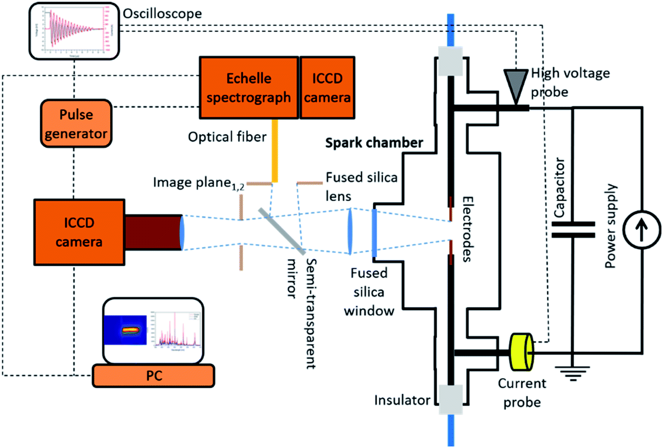 | ||
| Fig. 4 Schematic view of the experimental setup used for the in situ OES-based monitoring and imaging of a spark discharge nanoparticle generator. | ||
Although SDGs are most commonly operated in argon or nitrogen, pulsed discharges are also widely applied for producing NPs under a liquid environment.163–165 The working liquids usually consist of hydrogen, which allows for the application of the well-established methodology for deriving the electron concentration via the Stark-broadening of H lines.166,167
As it was mentioned earlier, another type of gas discharge used for nanoparticle generation – both in gas and liquid – is the thermal arc plasma.78 Arc discharge NP generators (ADGs) have the advantage over SDGs that due to the continuous regime and hence the lack of a capacitor and high voltage charging power supply, an even simpler and cheaper technical design can be realized.168 ADGs are characterized by high particle yield and very good scalability, however the particle sizes are typically considerably larger than that of spark-produced NPs and its applicability for producing high purity and multielement particles is also limited.168 From the point of view of spectroscopic measurements, arc plasmas have an even more established historical background, on which the monitoring of ADGs can be based.50 Generally, this includes all those plasma diagnostic techniques discussed in Chapter 2.2. and utilized for SDGs. However, due to the different plasma characteristics there are additional methods which can be employed. One important distinction from sparks is that – depending on the exact experimental conditions – the emission spectrum of the arc consists of a continuous background originating from the blackbody radiation of the electrodes.161 This can be simply exploited for temperature estimation in addition to other – already described – techniques, such as the Boltzmann plot and line-intensity-ratio methods, or for electron concentration measurements based on the Stark broadening.169,170 In ADGs operating under different experimental conditions molecular bands of the ambient nitrogen gas was observed in the spectrum, the intensity variation of which along the arc plasma was correlated to the properties of the produced nanostructures.169 Similarly, in case of underwater or submerged arcs, the features of the temporally resolved emission spectra were used to assess the peculiarities of the electrode erosion process and the degree of dissociation of water in the vicinity of the anode.171
In the previous paragraphs, the importance of spatial and temporal resolution in OES-based monitoring of arc and spark plasmas was pointed out and appropriate methods have been reviewed. These approaches mostly used well-localized signal collection with variable spatial positioning combined with a spectrograph. However, spatial resolution can be achieved in a single step by employing an imaging camera with appropriate optical filters. Bachmann et al. have proposed a method for obtaining the temperature distribution of a free-burning arc plasma, based on the simultaneous imaging of the plasma at two carefully chosen wavelengths.172 The experimentally acquired data was processed by using an LTE plasma model to derive the plasma temperature. Abel inversion of the data was used to reconstruct the radial distribution of the arc plasma column. A detailed assessment of the potential sources of errors and uncertainties was also provided.
In addition to the detection and analysis of the light emitted by the discharge plasma, the in situ monitoring of the particle generation has been also approached via laser-based methods. Santra et al. have shown theoretically that NPs can be detected via Rayleigh scattering spectroscopy during arc synthesis, along with the continuous monitoring of the evolution of the particle population.173 Rayleigh scattering spectroscopy is based on the probing of the electronic polarizability of particles interacting with a laser beam. Since Rayleigh scattering is elastic, this technique has the advantage over for instance Raman spectroscopy that the signal levels are orders of magnitudes higher.173 Another technique, which pushes down the detection size limit to the atomic scale and applicable to the in situ monitoring of arc synthesis is the coherent Rayleigh–Brillouin scattering (CRBS). CRBS is originally a laser-based gas detection technique, which was adapted to NPs and experimentally validated by Gerakis et al.174 CRBS relies on the creation of an electrostrictive grating and the probing of the velocity distribution in a medium via a four-wave mixing process. According to Gerakis et al. this technique can be effectively used to detect NPs in situ in volumetric particle generation methods, such as arc synthesis.174 The formation of arc-produced carbon nanostructures was also monitored in situ by using laser-induced incandescence measurements and simulations by Yatom et al.175 The viability of their approach was demonstrated via the recognition of two spatially separated group of particles with distinctly different sizes, having different role in the arc-based NP formation process.175 At higher laser fluences the particles can be effectively vaporized, which facilitates their in situ investigation by means of aerosol mass spectrometry. The successful application of this technique for investigating spark-generated NPs has been demonstrated by Nilsson et al.153
As it was mentioned at the beginning of this chapter, spectroscopy-based methodology briefly overviewed here are mostly applicable to thermal plasmas, where most of the LTE-based plasma diagnostic calculations can be carried out. However, OES-based techniques are involved in the investigation of cold plasmas as well. Particle generation by cold plasmas (produced by e.g. filamentary discharges or dielectric barrier discharges)176 can also be monitored by spectroscopic means. Due to the relatively low gas temperature molecular spectral bands are usually observable. The gas temperature can be determined by simulating the molecular spectrum and finding the best fit of its measured counterpart.177–179 Processing the experimentally acquired data is usually carried out by dedicated purpose-made software and scripts but commercial software is also available for fitting the spectra of several transitions observed in plasmas and for calculating the corresponding temperatures.180
2.4. Other generation techniques
In the previous subchapters we have briefly reviewed the laser- and plasma diagnostic techniques used for monitoring NP generation in plasma-based methods of high relevance from the point of view of applications. There are other additional particle generation methods as well, where the applicability of laser- and plasma diagnostic monitoring has been demonstrated. An example for such techniques is the continuous laser vaporization, which – unlike pulsed laser ablation – employs a continuous wave, usually CO2 laser to vaporize a precursor, predominantly for producing carbon nanotubes.181 Similarly to the monitoring of flames, CARS, LIF, and LII have been employed for the in situ monitoring of temperature, intermediate concentration, as well as the assessment of the particle formation process.182 In a similar, laser-based particle generation scheme, the applicability of in situ LIBS has also been demonstrated to monitor the properties of the generated particles. Picard et al. employed aerodynamic focusing of the NPs under vacuum in order to eliminate the contribution of the background gas from the LIBS spectrum.183 Low-temperature, low-pressure reactive plasmas are also successfully used to generate nanostructures,184,185 the formation of which can be monitored by laser spectroscopic approaches. Hundt et al. have employed quantum cascade laser absorption spectroscopy for the real time monitoring of the variation of the acetylene concentration in an Ar/C2H2 plasma during nanostructure synthesis in a radio frequency (RF) plasma.186 Leparoux and coworkers have investigated the synthesis process of graphene nano-flakes in Ar/H2/CH4 RF inductively coupled plasmas by using in situ OES.187,188 The acquired emission spectra allowed for the determination of the gas temperature from the C2 Swan band, which could be correlated to the particle generation conditions. A recent review on the monitoring of non-thermal plasmas used for NP synthesis has been published by Mangolini.189Particle generation techniques overviewed in the previous subchapters in context of real-time laser- and plasma spectroscopic process monitoring employed various types of precursors (solid, liquid, gas), in different media (liquid, solid, vacuum), but both included plasmas to initiate particle formation. However, laser spectroscopy has been also used to monitor wet chemical NP synthesis. Haber and coworkers used in situ second harmonic generation (SHG) and extinction spectroscopy to monitor the growth dynamics of seed-mediated gold and gold–silver core–shell NPs,190,191 which demonstrates the even wider possibilities of laser-based NP monitoring approaches.
3. Nanoparticle detection and characterization
3.1. Importance, driving force and overview
As it is known, the size and structure of nanomaterials are mainly responsible for their novel properties (electric, chemical, magnetic, optical, etc.), so naturally the characterization of nanomaterials has become the subject of intense research in the past couple of decades. Unfortunately, the fact that their size and structure critically determine their characteristics also makes the assessment of their physico-chemical properties (or structure–function relations) challenging, because their synthesis is prone to reproducibility problems and generally produces polydisperse particles, frequently with a broad distribution and defects. In addition to this, their characterization needs a comprehensive analytical approach, which also dictates the knowledge of limitations of the different techniques. As nowadays nanoparticles are being synthesized and used at an industrial scale, also including medical applications,192,193 it has led to their inevitable appearance in the environment, which in turn generated an urge for the development of sensitive and credible techniques for their detection.Since there is no universal characterization method that could simultaneously determine all important NP parameters, typically the use of complementary techniques is required. NP systems can be investigated in powder or suspension form but in certain cases the dissolution of particles is needed. Here follows a brief overview of the NP characterization methods. Further information about these techniques and their application in various media can be found in specific reviews and books.13,14,194–199
Electron microscopy techniques represent one of the most frequently applied group of NP characterization methods. Scanning electron microscopy (SEM) utilizes a well-focused electron beam that scans the surface of the sample and reflected electrons are used for imaging, while in transmission electron microscopy (TEM) a thin (typically less than 200 nm) sample interacts with the electron beam and the transmitted electrons are collected. Their popularity is derived from the fact that through “visualizing” NPs, a wide set of important characteristics can be determined, such as particle morphology, size distribution, degree of aggregation and – using a high-resolution apparatus – even crystal structure.
Scanning probe microscopes move a very sharp tip across the solid sample surface. In scanning tunneling microscopy (STM), DC voltage is applied between the conducting sample and the tip and the tunneling current, which is formed if the distance of the two object is very small (nm scale), is monitored. Atomic force microscopy (AFM) is based on electrostatic interactions between the atoms of the tip and the sample. Both STM and AFM allow for an atomic scale resolution imaging, hereby providing information on the morphology of nanomaterials. They can even be utilized to create structures in the sub-nano range by manipulating atoms or molecules on the sample surface.200,201
Due to different electromagnetic radiation–matter interactions, a great number of NP parameters can be studied by X-ray techniques. Complementing electron microscopy with energy-dispersive X-ray (fluorescence) spectroscopy (EDS or EDX) the elemental composition and its distribution in single NPs can be determined. Small angle X-ray scattering (SAXS) provides information about the size and size distribution, shape, and specific surface area of NPs. X-ray diffraction (XRD) probes ordered structures (crystal planes); hence the crystal structure, lattice parameters and crystallite size of the investigated nanomaterial can be determined. X-ray photoelectron spectroscopy (XPS) utilizes the photoelectric effect to perform surface analysis with an information depth of 2–10 nm. XPS is capable of the investigation of electronic structure, elemental composition, and oxidation states of elements in the surface of nanomaterials and its contaminants. Using appropriate data evaluation, particle size, single and multiple coatings, shell thicknesses and surface functionalization of NPs can be studied.202
UV-visible absorption spectroscopy is a simple and low-cost but not very selective characterization method which utilizes that the optical properties of NPs significantly depend on the size, shape, number concentration and degree of aggregation of the particles. NPs with intensive localized surface plasmon resonance in the UV-visible range (e.g. Au, Ag, Cu) are particularly often studied by this method.203 Infrared spectroscopy (IR) can also be utilized for certain nanomaterial characterization aims. The position of infrared absorption bands bears information on nanoparticle–biomolecule conjugation, conformational states, and secondary structures of the bound proteins.204
Atomic spectroscopic analytical techniques are widely used for nanoparticle detection and characterization. This is due to that their high selectivity permits the analysis even in complex sample matrices and their high sensitivity allows the investigation of small nanoparticles present at very small amounts. Inductively coupled plasma mass spectrometry (ICP-MS)205 and graphite furnace atomic absorption (GFAAS) techniques,206 should be mentioned as particular examples, traditionally exploited for the determination of the composition and mass concentration of nanodispersions.
In this chapter, we will focus on the NP characterization and detection techniques which are based on laser and plasma spectroscopy. Due to the vastness of the field, this overview obviously cannot be complete, but we will attempt to present the actual trends, relevant methodologies, and application examples. In the following sub-chapters, we organized the discussion according to the spectroscopic detection principle (e.g. absorption, emission, mass spectroscopy, etc.).
3.2. Techniques based on the interaction of nanoparticles with laser beams and plasmas
Laser–particle and plasma–particle interactions play a central role in techniques used for the detection or characterization of nanoparticles. These analytical techniques are specifically based on the light absorption, scattering or fluorescence of particles or on the detection of emission of photons or chemical species/fragments released (emitted) by the particles upon their interaction with a laser beam or plasma.The nature of the interaction involved in the measurement as well as the analytical benefit/information obtained vary among the techniques involved. A range of laser or plasma based analytical measurement techniques associated with NP detection and analysis are in use today; Table 1 provides an overview of the most important ones.
| Name of technique | Type of interaction | Principle of measurement | Analytical benefit/information |
|---|---|---|---|
| Laser-induced breakdown spectroscopy (LIBS) | Laser–particle and plasma–particle | Detection of characteristic light emission generated during the breakdown (or the vicinity) of particles in the LIB plasma | Detection of the presence of NPs and estimation of the composition/size/concentration of NPs dispersed in gaseous samples |
| Signal enhancement for liquid or solid samples (NELIBS) | |||
| Inductively coupled plasma mass spectrometry (ICP-MS) | Plasma–particle | Statistic evaluation of detected MS signal peaks caused by the breakdown of particles in the ICP plasma | Detection and detailed characterization (e.g. concentration, composition, size, structure, shape, density, porosity, etc.) of NPs dispersed in gaseous or liquid samples |
| Laser ablation inductively coupled plasma mass spectrometry (LA-ICP-MS) | Laser–particle and plasma–particle (at different locations) | Laser ablation of a solid sample in the vicinity of NPs, followed by the ICP-MS analysis of the ablated matter | Imaging of the spatial distribution of nanoparticles within solid samples |
| LA-ICP-MS signal enhancement | |||
| Laser desorption-ionization mass spectrometry (LDI-MS) | Laser–particle | MS detection of species/fragments released (evaporated/desorbed) from NPs upon their excitation by intense laser light | Analysis of the composition of particles |
| Laser-induced fluorescence (LIF) | Laser–particle | Detection of characteristic light emission generated during the laser excitation of particles (fluorescence) | Determination of the distribution, characteristic size or composition of NPs dispersed in a gas (aerosol) |
| Photoacoustic spectroscopy (PAS) | Laser–particle | Detection of characteristic light absorption of particles | Determination of the type or composition of NPs dispersed in gaseous or liquid samples |
| Nanoparticle tracking analysis (NTA) | Laser–particle | Image-based detection of light scattered by particles (can be combined with detection based on LIF) | Determination of the characteristic size and concentration of particles dispersed in a liquid |
| Dynamic light scattering (DLS) | Laser–particle | Image-based detection of light scattered by particles | Determination of the characteristic size and concentration of particles dispersed in a liquid |
| Laser-induced incandescence (LII) | Laser–particle | Laser heating of aerosol particles and detection of the subsequent thermal emission produced | Determination of the characteristic particle size and volume fraction of particles in the observed spatial region |
The interaction of nanostructures with light is a complex topic (essentially it encompasses the whole revolutionary field of nanophotonics) and therefore the discussion of its details is way beyond the scope of this chapter. Here, we would only like to point out to some of the specifics of laser–particle interactions relevant in laser and plasma spectroscopy. One aspect clearly involves the excitation of the surface plasmons (oscillations of free electrons) of metal or alloy NPs. Plasmonic resonances can be exploited in laser spectroscopy by generating signal enhancement (amounting to several orders of magnitude), as is discussed in the examples of SERS or NE-LIBS spectroscopies, in Chapters 4.3.2. and 4.3.3. Laser light, especially Q-switched giant-pulses, carry huge electrical field strengths (e.g. 109 to 1011 V m−1) which when interacting with the very high curvature NPs, can easily produce field emission of electrons. These can serve as seed electrons that lower the laser ablation and laser-induced breakdown thresholds, thereby facilitating analytical techniques such as LA-ICP-MS or LIBS.207 Light scattering is a well-known optical phenomenon during which the incident light perturbs electrons in the structure to form oscillating dipole moments that re-emit the light in different directions. The intensity and direction of this scattered light depend both on the incident wavelength and specific properties of the structure. Light scattering is exploited for the size and concentration characterization of NPs in techniques such as DLS and NTA. Furthermore, it has been shown recently both theoretically and experimentally that if the light interacts with subwavelength structures (NPs) then superscattering can occur. This effect, in the present context, may result in a further decrease of the size detection limit of certain NPs.208 Absorption of laser light by aerosol particles is exploited in techniques such as laser desorption and ionization mass spectroscopy (e.g. MALDI, or LDI-MS), laser-induced fluorescence (LIF) and photoacoustic spectroscopy (PAS) for the characterization of the chemical composition and size distribution. Individual particles can also be trapped optically and then interrogated by laser beams.209
In the context of detection and characterization, the interaction of nanostructures with plasmas is typically a breakdown process. The analysis of nano- and microparticles (including suspensions and aerosols) using plasma spectroscopy basically falls within the interest of atomic spectroscopy, where the plasma serves as the high temperature atomization/ionization source. Major examples include ICP and LIB plasmas. Detailed experimental and numerical simulation studies are available in the recent literature which investigate the propagation and decomposition of particles introduced into analytical plasma sources, as well as the influence of instrumental conditions on the analytical signal formation (e.g. ref. 210–212). Of particular importance here is single particle ICP-MS, discussed in detail in Chapter 3.3.6.1., which is rapidly becoming a popular and versatile nanoparticle characterization technique.
3.3. Methodology and applications
Instruments falling in this category are based either on the measurement of scattering intensities at various spatial locations (OPC, LD, MALS) and/or as a function of time (DLS), or follow particle movement (PTA). The theory of light scattering by spherical dielectric particles with isotropic optical properties have been worked out a long ago (Mie) and later expanded to other symmetrical shaped particles. At the same time, no exact mathematical solution exists for the description of scattering intensity distributions for arbitrarily shaped and/or optically anisotropic particles, thus in these cases, approximations based on matrix and numerical methods are used (e.g. ref. 220 and 221). For this reason, data evaluation in laser scattering particle characterization techniques require an a priori assumption about the shape of the particle and cannot work with irregular and mixed-shaped particles. In addition, in a liquid medium, these techniques generally require a suitable refractive index contrast between the medium and the particle, a strong dilution, as well as a reasonably monodisperse sample, thus prior separation by e.g. size exclusion chromatography (SEC) or field-flow fractionation (FFF), ultracentrifugation, etc., is often needed. Complex samples with strong background fluorescence and scattering from medium-sized molecules can cause difficulties. The smallest particle sizes detectable are typically in the 10–40 nm range, but this value strongly depends on the sample.134,213
Today, DLS and NTA are the two most popular particle characterization scattering techniques in suspensions, but NTA has distinct advantages over DLS in the case of NPs. Since DLS is an intensity weighed methodology which measures the fluctuations in scattered light intensity and correlates it to the particle hydrodynamic diameter via the correlation function and the Stokes–Einstein equation, therefore size distribution curves are heavily weighted towards larger particle sizes. As opposed to this, NTA uses a camera to individually identify and track the motion of each particle in the suspension. This gives a better-balanced size distribution curve; only 50% difference in particle diameter is needed for successful size resolution, whereas a ca. threefold difference is required by DLS – this makes NTA superior for the analysis of polydisperse samples. In addition, NTA is inherently capable of determining the particle concentration.38,134
LII is particularly suitable for the detection of aerosol NPs if the particle has a large extinction, which is true for carbonaceous particles (soot). Incipient soot particles are close to spherical and are small (1–10 nm), mature soot is composed of primary particles of 10–50 nm in diameter with a fine structure. These primary particles are then covalently bound into non-spherical aggregates of tens to hundreds of nanometers in size. Soots are also very suitable LII measurement subjects, as they have a very high (in excess of 4000 K) sublimation temperature and an appreciable imaginary part of the refractive index. Therefore, in environmental and industrial applications, LII has been used extensively for the qualitative measurements of temporal and spatial distributions of soot, but quantitative measurements of volume fractions and primary particle size have also been attempted.52,222
Apart from soot, engineered NPs have also been measured by LII due to the increasing interest in the synthesis of nanoparticles in the gas phase. In situ measurement of particle sizes is of particular interest because it offers the possibility of process monitoring/control. In this context, successful analysis of carbonaceous and non-carbonaceous engineered NPs have equally been reported. The list includes e.g. carbon nanotubes,223,224 metal-oxide (e.g. TiO2, Mn- and Fe-oxides)225–227 and metal/metalloid (e.g. Ag, Cu, Ti, Mo, W, Ni, Fe, Si)228–230 NPs. However, the transfer of the accumulated knowledge in the LII analysis of carbonaceous particles to various inorganic NPs are not without challenges. For example, plasmonic resonances in aggregates of noble metal NPs can experience a highly non-uniform heating. There is also a large uncertainty associated with values of the thermal accommodation coefficient, a central parameter in LII data evaluation, for most combinations of non-carbonaceous particle material and ambient gas. It was recently suggested that molecular dynamics calculations231 might be used to tackle this problem.
Laser-induced incandescence is commonly linked to the measurement of nanoaerosols, but investigations that focus on the measurement of suspensions also occur in the literature. This interest is somewhat limited though, since there are commercial laser scattering-based instrumentations available for this purpose (e.g. DLS, NTA). As an example, the study of Sommer et al.232 can be mentioned here, in which the authors investigated the pulsed-LII-signal decay times of carbon-black nanodispersions and found a linear correlation with the primary-particle size determined by electron microscopy. There are also reports about black carbon NP measurements in rain and snow samples (e.g. ref. 234).
Utilizing the localized (spatially resolved) analysis capability of LIBS, its application to nanoaerosol (ultrafine particulate matter) or NP detection and characterization has been successfully demonstrated in solid, gas and liquid phases over the years. For example, sub-micron or nanoaerosol particles, both on-line (free-stream, e.g. ref. 33) and off-line (following collection on filters, e.g. ref. 237) aerosol analysis approaches were tested in the literature, since LIBS was first employed for aerosol analysis in the 1980s.238 Among others, important contributions to the field were made by Hahn and co-workers239,240 as well as by Noll and co-workers,241,242e.g. with respect to sampling statistics, triggering, assessing the upper size limitation on the complete ablation of NPs, etc. Aerosol analysis by LIBS in general has been recently reviewed in ref. 240 and 243.
Indicatively, three noteworthy directions of recent LIBS efforts in the field of nanomaterial analysis should be mentioned here: (i) selective analysis of aerosol NPs by low intensity pulses, (ii) characterization of optically trapped single NPs or nanodroplets, and (iii) mapping the distribution of NPs in biological matrices. The following sections outline the progress in these fields.
3.3.3.1. Selective analysis of aerosol nanoparticles. When studying TiO2 nanoaerosols using LIBS, Zhang et al. observed low-intensity atomic emission spectra from Ti atoms without any macroscopically visible spark although the used laser pulse energy was significantly lower (2–35 mJ) than typical values necessary for LIBS aerosol analysis.244 At the same time, no spectral lines from the ambient gas (nitrogen) could be observed, indicating that there was no gas-phase breakdown. After a detailed investigation, the authors concluded that under such conditions, a nanoplasma is created which only breaks down the NPs. It was also observed that the atomic emission signal grows with the increase of the size of nanoparticles, reaching a maximum at around 6 nm (for TiO2 and 532 nm laser wavelength). The methodology was named low-intensity phase-selective LIBS (PS-LIBS). Two significant advantages of the technique were articulated by the authors: (i) the very short (ns range) lifetime of this nanoplasma allows for the use of similarly short gate-delay times, (ii) the emission spectrum is free from gas lines; therefore, it can be used for the detection of NPs or for the selective monitoring of NP synthesis processes. These advantages were experimentally exploited in follow-up metal-oxide NP aerosol studies by the same group245–247 and even a theory for the mechanism of absorption–ablation–excitation laser-nanoparticle cluster interactions was developed.248 It was established that the threshold irradiance that triggers the formation of nanoplasma is about six times higher for a 1064 nm excitation wavelength than for 532 nm, resulting in an emission intensity that is nearly 100 times lower in the former case. Based on this observation and the ablation model proposed by the authors involving two-photon excitation of electrons in the conduction band of the metal-oxide particles, it was suggested that an excitation wavelength tuned to above the bandgap of the material of interest should be used.245,248 Tse et al. also proposed and successfully demonstrated245,249 that the resonance signal enhancement methodology (RELIBS, originally introduced by Cheung et al.250,251), which involves the use of an additional delayed excitation laser pulse tuned to one of the electronic transitions of a major constituent of the sample (here: particle), can be exploited to produce a more than two orders of magnitude increase of the inherently weak PS-LIBS signals.
3.3.3.2. Characterization of optically trapped nanomaterials. Aerodynamic focusing252 and optical trapping253 of fine and ultrafine aerosol particles, followed by an investigation of the characteristics of individual NPs is an upcoming analytical approach in the last decade, but LIBS has been applied to trapped NPs and nanodroplets only most recently. The Laserna group in Malaga, Spain, pioneered this approach34,35,254,255 and demonstrated that LIBS possesses the attogram-level detection power necessary for such an analytical task.
The Spanish researchers employ their proprietary sample introduction methodology, named optical catapulting (OC), which is based on the ejection (mobilization, suspension) of particles deposited on a glass slide into the surrounding gas, initiated by a laser pulse delivered to the backside of the slide, to put the particulate material under inspection in aerosol form. A cw laser beam at 532 nm is then used to isolate and manipulate individual NPs from the aerosol (optical trap, OT), which are subsequently analyzed by using a 1064 nm nanosecond laser pulse for LIBS (Fig. 5). Once catapulted, the dynamics of particle trapping depends both on laser beam characteristics (power and intensity gradient) and on particle properties (size, mass, and shape). The utilized long working distance (low numerical aperture) microscope objective to focus the low power (140–250 mW) cw trapping beam allows for a very stable holding of the NPs at atmospheric pressure over a large length (e.g. 5 mm).34,254,255 In the latest study of the authors,35 an enhanced sampling strategy, based on using skimmer-like cones, was introduced to double the sampling throughput of OC-OT-LIBS technology for single NPs.
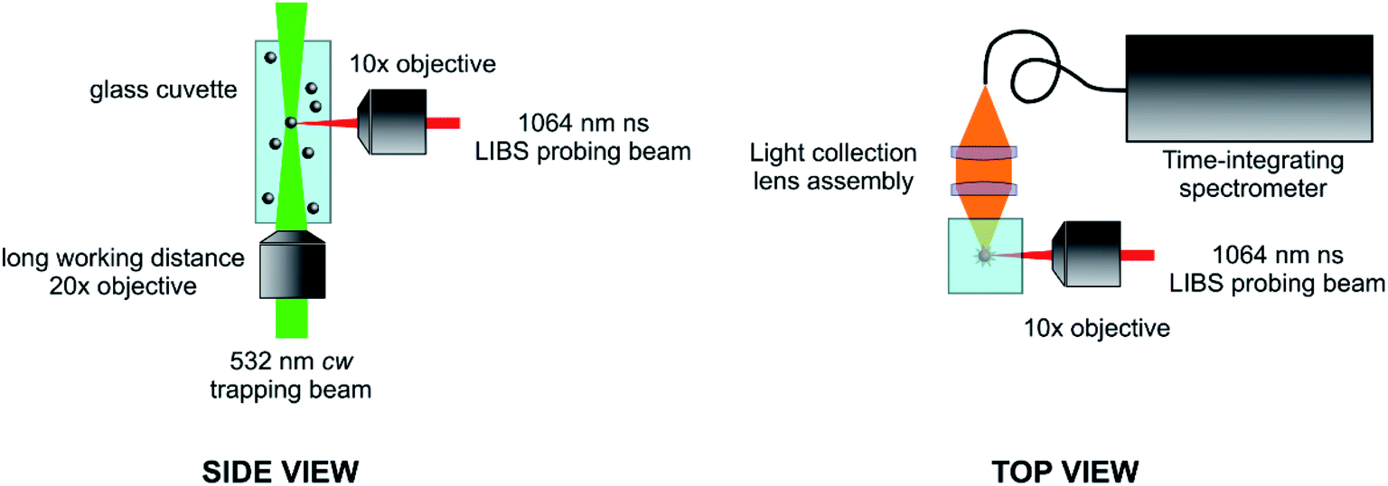 | ||
| Fig. 5 Scheme of an experimental arrangement for LIBS analysis of optical trapped single nanoparticles. | ||
Detailed high-resolution imaging with an ICCD camera provided visual feedback on the particle manipulation. Trapping efficiency was defined as the number of catapulting events resulting in a particle entering the optical trap and remaining occluded for a period long enough to proceed with LIBS characterization. Trapping was considered stable once no confined particle–aerosol collisions could be observed in the camera image. 76–93% trapping efficiencies, half of which were single particle events, were achieved in the studies. Interestingly, an inverse relationship between the emission intensity and particle mass was found, which allows for LIBS measurements with unprecedented sensitivity. With the OC-OT-LIBS, the Laserna group successfully recorded good S/N LIBS spectra of individual 100 nm Al2O3,254 25 nm Cu,34 400 nm graphite255 and 90 nm copper-oxide35 NPs. The sample introduction and analysis only took 3–6 minutes.
Most recently, Niu et al. proposed an optical trapping approach based on the use of a hollow cw laser beam, and successfully demonstrated that OT-LIBS can be applied for the quantitative determination of metal concentrations in individual, 2 μm black carbon aerosol particles.256 In other studies, nL volume droplets and 1–3 micrometer aerosol particles were also successfully trapped and individually analyzed by LIBS. Järvinen et al.257 used an electrodynamic, whereas Meneses-Nava et al.258 an acoustic levitator for the trapping of particles. Since all the above three technologies can spatially constrain aerosol particles to a very small, μm-wide range, they are expected to be applicable to ultrafine (nano) particles as well.
3.3.3.3. Mapping of the distribution of NPs in biological samples. LIBS was recently also successfully used to assess the accessibility of NPs to and distribution of nanoparticles in plants and animal tissues. Although there are other techniques capable of providing spatially better resolved chemical maps (e.g. SEM or TEM), but the advantage of LIBS is that it can also be applied to large samples and it requires no labeling. The compatibility of the LIBS setup with standard optical microscopes also provides a potential to obtain multiple images of the same biological tissue with different types of response including elemental, molecular, or cellular. It is noteworthy that – in contrast to general LIBS solid sample analysis – biological tissue samples need to be prepared for LIBS analysis. Although there is no standardized procedure for this, but it generally involves embedding in epoxy. For soft tissues, a prior dehydration is also needed. Of course, there are variations in the approaches used depending on the tissue type – in the case of nanoparticle detection, thin sectioning (into 10–40 μm slices) was also found to be necessary. Further details, e.g. sample preparation, instrumental requirements, data evaluation, on LIBS imaging of various species in biological samples can be found in related recent reviews.236,259–261
The research group of Motto-Ros is the pioneer and driving force behind LIBS elemental imaging and NP distribution research in human and animal soft tissues. Most of their investigations serve with information for preclinical medical studies and kinetic biological studies. In 2012, the research group proposed a methodology for the elemental imaging of metal-based NPs in frozen murine biological tissues.262,263 The distribution of Gd NPs was imaged in two dimensions at the scale of an entire organ (i.e., kidney or liver). Kinetics studies, in which NPs were injected into animals, were also supported by LIBS NP detection, by screening the organs of elimination at different times after administration of metallic NPs. In 2014, the spatial resolution of the instrumentation was improved to 35 μm, which enabled the observation that Gd-based NPs were predominantly localized in the renal cortex at early time points before being progressively accumulated in the medulla; the effective renal clearance of Gd NPs was observed one week after the injection.263–266 Motto-Ros et al. also used LIBS to investigate the tumor-penetration of NPs. From this point of view, the behaviour of Gd/Si-based267 and Au-based268 NPs were investigated on paraffin-embedded specimens made from monkey and mice pancreatic and glioblastoma tumor-bearing models. LIBS analysis clearly indicated the presence of metal NPs both in the center and at the periphery of tumors, which confirmed previous results obtained with magnetic resonance imaging (MRI). The lateral resolution achieved in the above studies was strongly impacted by the sample preparation and sample type: 40–100 μm resolution was achieved for cryo-sections,263 whereas a resolution of 10 μm was achieved for hard epoxy-embedded samples. A 3D extension of the conventional 2D LIBS imaging method was also developed, the applicability of which was tested both via volume reconstruction and direct depth-resolved analysis,269 working in a complementary way with conventional imaging techniques, i.e., transmission electron microscopy and fluorescence microscopy,266 studying the distribution of gold-based NPs in various organs such as the kidney, liver, and spleen.270
The first visualization of NP distribution in plant tissues with LIBS was published in 2017 by Czech researchers from Brno, who are still at the forefront of this research direction since then. In their first study, the distribution of Ag ions and ultra-small Ag NPs in Vicia faba (faba bean) root cross-sections were detected with a resolution of 50 μm.271 In follow-up studies, Raphanus sativus L. (radish), Lemna minor L. (common duckweed), Sinapis alba L. (white mustard) were also used as test plants and the uptake and translocalization/accumulation of CdTe quantum dots,272,273 as well as Y- and Er-containing photon-upconversion fluorescent NPs.274 The studies revealed that the NP uptake rate is very slow and in certain plants there are differences in the way NPs and metal ions are accumulated. The obtained information was found to be very valuable in plant toxicity studies.
It is essential in PAS that the release of heat from the particle occurs fast enough not to interfere with the modulation frequency, but this condition can be met easily for NPs, for which the temperature increase is typically on the order of millikelvins, and the thermal relaxation times are on the order of ns only. It is also generally important that the particle is dried before PAS measurements otherwise a loss of signal can occur due to mass transfer (release of volatile compounds); but again, this is less of a concern for NPs due to the tiny temperature increase.277
Unfortunately, the very small mass and ΔT of NPs also means that their PAS signal is very small, in fact it was shown to rapidly decrease with the particle size.278 Due to this reason, PAS is still far more commonly used for the characterization of microparticles rather than nanoparticles. However, using signal amplification (e.g. quartz-enhanced or optical cavity-enhanced PAS) and/or trapping by optical tweezers, the detection and characterization of nanodroplets279 and single NPs (800 nm or less)278,280,281 have been recently successfully demonstrated.
The one type of larger NPs (around or below 100 nm in diameter) that can be efficiently detected by PAS is soot or black carbon (these two names are often interchangeably used, see ref. 282), which have great importance in environmental science.280 In recent years, the internationally recognized PAS research group of Bozóki, Szabó and Ajtai has published several reports about successful method developments and applications for these atmospheric nanoaerosols (e.g. ref. 283–285).
Particle characterization (e.g. identification, classification) style of applications of LIF, which fall more under the category of spectroscopy, are rare. One such awakening technique is LIF-LIDAR (light detection and ranging). Absorption LIDAR for chemical analysis is a well-established long-distance stand-off laser spectroscopy method for atmospheric gas and aerosol analysis, which monitors the time-resolved attenuation of a laser pulse backscattered from distant aerosol particles occurring when the pulse traverses the space between the laser source and the particles.296 LIF-LIDAR is a variant of this technique, which uses the fluorescence emission signal of the aerosol particles for their detection and characterization. It has been recently demonstrated by a few publications that LIF-LIDAR can classify atmospheric bioaerosol types (e.g. fungi, pollen, bacillus cells, etc.) based on their fluorescence emission spectra, even when their concentration in the air stream is as low as a few particles per liter.297–299 Obviously, both a low aerosol number concentration and a long optical pathlength (the latter due to the very small collection angle) work against the minimum detectable particle size. While most of the bioaerosol particles measured in these studies were in the tens of micrometer range, but some (e.g. bacillus cells) were only about 1 μm in diameter, hence there is a promise that this approach can be developed into a nanoaerosol characterization technique soon.
There are several publications that describe the application of MS to NP characterization. Excellent review papers on this topic are also available.300–302 Although other approaches could have been also adopted for the classification of the related literature (e.g. according to the particle characteristics determined), but here we employed a four-tier, instrumentation-oriented strategy. In the first, largest, section, we overview the progress in the so-called single particle ICP-MS (spICP-MS) sub-field, which is perhaps the most versatile and has clearly produced the fastest growth in the past decade, with over several hundreds of papers in total.36 Naturally, this approach is primarily focusing on the analysis of engineered inorganic NPs dispersed in fluid media. The second sub-chapter gives an overview about the applications in which laser-ablation (LA) is used as a spatially resolved sample introduction approach for studies on the distribution of NPs in solid samples (similarly to LIBS-based approaches already discussed in Section 3.3.3.). In the third section, we briefly discuss the sub-field which relies on the combination of some separation techniques with ICP-MS. These allow for the analysis of polydisperse colloid systems and structurally complex nanosystems hardly accessible for other characterization approaches. Finally, some attention will be given to molecular (organic) MS applications too, which deal with the characterization of functionalized NPs (ligand coatings) or bio-nanoaerosols. Please note that, due to the scope of the present review, only the applications involving laser desorption/ionization (MALDI), or an ICP-MS detector will be discussed in the fourth chapter.
3.3.6.1. Single particle ICP-MS. Single particle ICP-MS (spICP-MS) is a novel technique capable for the investigation of individual nano- and microparticles in suspensions. The first application of spICP-MS was described in the articles of Degueldre et al. published303–306 between 2003 and 2006. In the early years, around 2010, the basic principles of spICP-MS (e.g. signal formation, data evaluation and calibration) was described by the research groups participating in early assessment of the capabilities of the technique.307–309 By the end of that decade, spICP-MS has already become an established and rapidly developing NP characterization technique which enables the routine determination of the presence, size, size distribution and particle number concentration of dispersed NPs in an element- and isotope-selective way. The different aspects of spICP-MS were already assessed in detail in a handful of reviews.36,37,197,310,311 The following section presents only the basic principles of the technique, recent developments, and applications.
One of the greatest advantages of spICP-MS is that wide-spread ICP-MS instruments equipped with a (single) quadrupole mass analyzer are suitable for the characterization of individual NPs without any hardware or software modifications. NP suspensions can be analyzed directly by spICP-MS, hence the dissolution of the particles can be avoided, and the sample preparation generally includes only dilution and filtering steps. It should also be highlighted that spICP-MS can distinguish between the dissolved and the particulate form of the analyte.307,312 Thanks to the low particle number concentration sufficient for the analysis (approximately 103 to 105 particles per mL), spICP-MS is a practical and convenient choice for the detection of NPs in environmental and biological media contrary to most other NP characterization methods.308
The basic concept of spICP-MS is that properly diluted NP suspensions are directly nebulized into the instrument, resulting in the presence of individual particles in separate droplets. Upon introduction into the plasma, these droplets/particles decompose (atomization and ionization) and the ion clouds of separate NPs are detected individually in time resolved analysis (TRA) mode. There are basically two possible approaches for the detection of single NPs by ICP-MS (Fig. 6). One – that was chronologically the first to be introduced into the literature – utilizes a longer dwell time than the length of the TRA signal of the particles (that is typically a few hundred to thousand μs (ref. 309 and 313–315)). Multiple times longer dwell times (e.g. 10 ms), though, can result in the co-detection of more than one NP during the same dwell time. The probability of this can be minimized by the dilution of the sample suspension but the measurement time also needs to be increased to maintain the necessary number of detection events for a proper statistical evaluation. Co-detection of NPs can also be avoided by decreasing the applied dwell time (e.g. to less than 1–5 ms), but in this case, the probability of splitting the NP ion clouds randomly reaching the detector is increased (peak splitting) which has a negative effect on the accuracy of the particle size determination. It is further hindered by the signal loss due to detector settling time.
 | ||
| Fig. 6 Representative ICP-MS signal (monitoring m/z197Au) due to 30 nm AuNPs (2.5 ×10 5 mL−1) acquired simultaneously for 2 s with (a) 10 ms dwell time (vendor software), and (b) 5 μs dwell time (home-built data acquisition unit). First zoom level shows several particle events in (c) and (d) for about 400 ms (for the highlighted section in (a) and (b)). Second zoom level (e) shows the temporal profile of a single particle's ion cloud identified with the home-built data acquisition unit in (d). Adapted from ref. 316. | ||
With the development of ICP-MS instruments, the utilization of dwell times shorter than the length of a particle event (high time resolution), e.g. 10–100 μs, became available. During data evaluation, the split particle signals need to be assigned and integrated. The advantages of this approach are that it can reduce the possibility of particle co-detection, lower the continuous background intensity (resulting in a better signal/noise ratio) and the possibility for the detection of multiple elements or isotopes in the same particle.317,318 On the other hand, the use of a lower dwell time also decreases the measured signals, which is critical for the quantitative measurement of NPs with a small size in the aspect of both the detection and the peak bordering.319
By performing the individual detection of NPs, a linear relationship can be drawn between the number of detected particle events (nP) and the particle number concentration (cP):
| nP = ηnebQtdwellcP | (6) |
For solid, homogeneous, spherical NPs, the correspondence between the intensity of a particle peak (IP) and the mass of monitored analyte in the particle (mP) can be described as:
 | (7) |
 | (8) |
To determine NP size, size distribution and particle size detection limits, the calibration of spICP-MS is needed, during which process the function relating the particle mass to detected signals is established. In practice, spICP-MS calibration can be performed in two ways, utilizing (i) standard NP suspensions or (ii) standard solutions containing the investigated analyte.306,308 Although some earlier studies used a linear function to fit calibration data, but in principle, the calibration function follows a cubic relationship between the particle size (diameter or radius) and the ICP-MS signal.306 This logical assumption is also supported by recent plasma modeling studies which proved that practically the whole NP ion cloud passes through the hole of the sampling cone under typical experimental conditions.210 Although the utilization of NP standards for spICP-MS calibration purposes is straightforward and less exposed to the effects of experimental variability, a notable limiting factor is the shortage in the commercial availability of monodisperse, well-characterized particle standards.
The application of standard solutions for spICP-MS calibration was first introduced by Pace and co-workers.308 An essential condition to use this calibration technique is that after the decomposition in plasma, analyte ions with the same elemental composition go through the same (or reasonably similar) processes until their detection in the cases of both NPs and the solute. The mass of individual NPs is calculated on the basis of mass flow of the solution:
| W = cstdηnebQtdwell | (9) |
In spICP-MS literature, the size detection limit is calculated as three or five times the standard deviation of the background signal.306,308,320 Size detection limits are typically around 10–40 nm for one component metallic NPs.36,321 There is also an upper limit for the NP size, as particles larger than a certain size do not spend enough time in the plasma for full decomposition and ionization.309,322 This upper size limit heavily depends on the studied element, but it can be estimated to be about a micrometer.
The main research goals related to spICP-MS sample introduction are to decrease the required sample volume and to achieve approximately 100% transport efficiency in order to obtain lower particle number detection limits. It also promotes calibration carried out using ionic standard solutions. Flow injection systems offer an attractive alternative for the introduction of NP suspensions. This is because by utilizing an injection loop of known volume, the total injected mass of analyte is also known, thus the determination of transport efficiency and sample uptake rate is not required for the measurement of the mass of NPs.323,324 Another possibility to achieve the highest possible transport efficiency is represented by microdroplet generator (MDG) sample introduction systems which can produce monodisperse droplets with a controlled volume and speed.325,326 Unfortunately, MDGs are more prone to contamination and clogging compared to pneumatic nebulizers, hence, several papers demonstrated the advantageous utilization of the combination of pneumatic nebulizers and MDGs.327–330 In these setups, MDG provided well-defined droplets of known dissolved ion concentration for calibration purposes and NPs were introduced by a pneumatic nebulizer via a dual-inlet system.
It was also shown that – like solution mode ICP-MS – spICP-MS is prone to certain interferences. The occurrence of non-spectral interferences in matrices containing carbon or sodium in high concentration can have a significant impact on NP signals, which unfavorably affects NP sizing.331,332 To tackle these undesirable effects, Telgmann et al. performed isotope dilution using 109Ag enriched standard solution to characterize Ag NPs in wastewater and river water matrices.333 Huang et al. successfully applied dissolved Rh as internal standard to accurately determine the size distribution of polydisperse CeO2 NPs in human urine, rat plasma and enzyme-digested rat liver tissue matrices that showed significant matrix effect.334 The already described pneumatic nebulizer plus MDG dual-inlet sample introduction system offers another possibility to overcome non-spectral interferences as calibration solutions are exposed to the same matrix effects as the investigated NPs.328,335 Spectral interferences and the effect of collision/reaction cell (CRC) technology on NP signals were also investigated in the literature of spICP-MS. Kálomista et al. proved the usefulness of the application of He collision gas to eliminate polyatomic interferences for the analysis of Cr2O3 and Fe2O3 NPs.312 The advantageous application of a “triple-quadrupole” (tandem) ICP-MS with a CRC was demonstrated in several papers as well. Bolea-Fernandez et al. characterized the size of SiO2 particles using H2 reaction gas and on-mass analysis, and achieved a 75 nm size LOD.336 For the analysis of titania NPs Tharaud et al. NPs suggested the use of NH3 reaction gas in calcium-rich matrices,337 while Candás-Zapico et al. demonstrated the superiority of the application of O2 reaction gas to decrease size detection limits in the absence of Ca in the sample matrix.338 Fe3O4 NPs were characterized by Rua-Ibarz et al. using an on-mass CRC technique using H2 and the authors developed a “pseudo resolution” sector field ICP-MS method for fast transient ion signal monitoring and to overcome the ArO+ spectral overlap with 56Fe.339
The multi-element detection capabilities of quadrupole-equipped ICP-MS instruments are limited due to their sequential principle of operation which also introduces a signal settling time when the mass analyzer is re-tuned. The detectable number of elements in a single particle is influenced by both instrumental parameters (e.g. gas flow rates,340 length of dwell time and settling time318) and NP properties (transient signal length through the particle size and the structure of the NP314). Even by utilizing μs dwell times, usually no more than a 3–4 analyte isotopes can be determined within a particle and at some cost of quantitativity of the results.341 ICP-MS instruments equipped with a time-of-flight mass analyzer offer a promising approach for the quasi-simultaneous multielement analysis of NPs (spICP-TOFMS). Naasz et al. demonstrated the utility of spICP-TOFMS by the multielement (Fe, Mo, Cr, Ni) analysis of composite nano-steel platelets.342 Multi-element fingerprinting was also shown to help in the differentiation of geogenic and engineered NPs.341,343,344
The versatility of spICP-MS was further increased by research groups developing methodologies and data evaluation processes to determine additional important NP characteristics beyond particle size distribution and number concentration. Kálomista et al. utilized microsecond range data recording and demonstrated that by comparing the transit time of the ion cloud of particle events, spherical and rod particle geometries can be distinguished (Fig. 7), moreover, the aspect ratio (the length to width ratio) of nanorods can be determined.313 High time resolution data was also exploited to gain information on particle structure; Kéri et al. developed a data evaluation method to discriminate mixed alloy and core–shell Au–Ag NP transient signals.314 Completing single particle detection with the data of particle external diameter obtained by another NP characterization method (e.g. DLS, NTA, SEM, TEM), the density and porosity of NPs can also be calculated.345–347 Sápi et al. utilized spICP-MS to determine platinum concentration of Pt/SiO2 nanocomposite decorated with ultra-small Pt NPs and highlighted the outstanding accuracy and precision of the spICP-MS technique by comparing its results to the ones obtained by other wide-spread NP characterization methods (TEM, solution mode ICP-MS, SEM-EDX, XPS).348
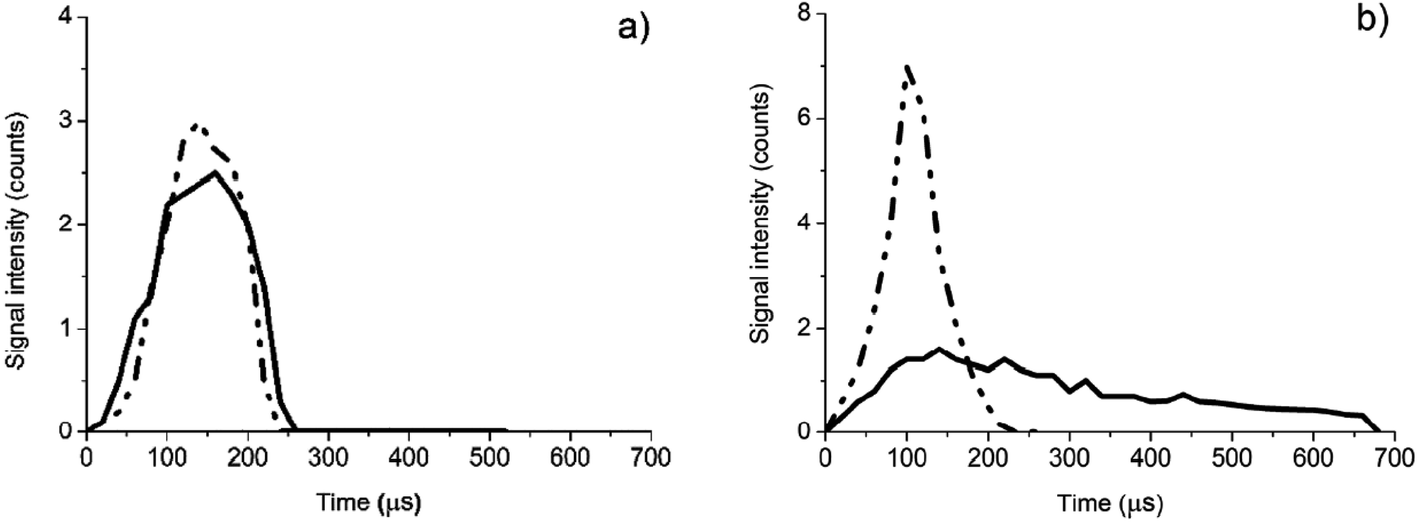 | ||
| Fig. 7 A comparison of the high time resolution signal profiles for 30 nm diameter spherical gold NPs (panel a) and for 2.63 aspect ratio gold nanorods (panel b). In each panel, the two extreme time profiles (with the shortest (dashed dotted line) and longest (solid line) durations observed) as averages for 40–50 particles are shown.313 | ||
The excellent matrix tolerance and sensitivity of ICP-MS instruments and low particle number detection limits of the single particle technique enable the characterization of natural and engineered colloid particles in quite complex matrices too. Environmental applications include the analysis of NPs in lake, river and sea water, wastewater, soil as well as sediment samples.311,349 NPs were also detected and characterized in human tissues,350 urine,351–353 blood,352,353 serum353 exhaled breath condensate,354 simulated gastric fluid355 and artificial sweat mixture,356 animal tissues and blood357–359 and in different parts of plants360–362 as well.
For risk assessment, the characterization of NPs in food products is an important task. NPs can accumulate in animals harvested as food from environmental sources. Zhou et al. applied spICP-MS for the characterization of metallic NPs in shellfish seafood and detected Y, La, Ce, Pr, Gd NPs in clams and Y, La, Ce, Pr, Nd NPs in oysters.363 Xu et al. also analyzed NPs in marine mollusks from an offshore aquaculture farm and demonstrated the bioaccumulation of Ag containing NPs in the investigated organisms.364 NPs can also stem from food additives, e.g. E 171 colorants of different products were proved to contain TiO2 NPs with particle size below 100 nm in significant amount.365–367 Loeschner et al. demonstrated the presence of Al-containing NPs in Chinese noodles, though, the origin of the particles (whether natural source, contamination of food storage/processing or additive agent) stayed unclear.368
The number of consumer goods that are intentionally fabricated with the addition of NPs to improve their attributes is also rapidly increasing. The potential of spICP-MS was demonstrated in the literature by the characterization of TiO2 NPs in sunscreens,369 Al2O3 and TiO2 NPs in toothpaste370 and Au and Ag NPs in consumer spray products.371 Mackevica et al. proved the release of Ag NPs from toothbrushes, and TiO2 NPs from textiles.372,373 Ntim et al. investigated TiO2 and SiO2 NP migration from ceramic cookware to foodstuff.374 Several studies prove the usefulness of spICP-MS for the analysis of the particles present in or released from industrial products as well. The release of nano and sub-micron particles was monitored from different painted surfaces,375,376 printed nanosilver circuits377 and nano-enabled pressure-treated lumber378 and their presence was demonstrated in tattoo inks379,380 as well.
The exploitation of spICP-MS for bioanalytics is also advantageous.381,382 For example, it was utilized for the individual detection of cells that is generally referred to as single cell ICP-MS (scICP-MS) in the literature. As cells are significantly larger than NPs, special sample introduction tools were developed and applied for scICP-MS to boost cell transport efficiency.383 The cell number concentration can be determined by the measurement of the (natural/spiked) major elements (e.g. P, Mg) of the cells384,385 and information can be obtained on the presence,386,387 bioavailability388 and uptake kinetics389 of different compounds and particles related to the cells. spICP-MS can also be exploited as a sensitive readout tool for NP immunoassay tags, where the analytical information originates from the proportionality between the frequency of the detected particle events and the concentration of the analyte labelled with NPs.390–392
Besides the above-mentioned applications, there are other special fields where spICP-MS has already revealed its potential. For example, the characterization of metallic NPs in non-aquatic media was carried out by Nelson et al. who investigated asphaltene samples diluted in o-xylene.393 Ruhland et al. detected Hg-containing NPs dispersed in tetrahydrofuran that originate from gas condensates of petroleum hydrocarbon samples.394 It was also demonstrated that inorganic gunshot residue contains NPs that can be analyzed by spICP-MS for forensic purposes.395 Fine (sub-micron and nano) particles were dispersed and detected by spICP-MS from electronic cigarette aerosols396 and paper printing and shredding process397 as well. The technique was assessed as especially favorable for the fast and sensitive probe for functional pore sizes of ultrafiltration membranes by investigating the retention of NPs.398
3.3.6.2. LA-ICP-MS. The main focus in this LA-ICP-MS application field is the imaging of the spatial distribution of NPs within a solid material, which is often of biological origin. The frozen or epoxy embedded sample is placed on a three-axis stage and by scanning the laser beam across the sample surface, the material is ablated, and the resulting aerosol is transported with a carrier gas flow into the plasma. A polymer, glass or metal tubing is used as a transfer line. Argon, helium or rather their mixture is used as carrier gas as the addition of He was found to be beneficial from the point of view of lateral resolution (due to a lower amount of ablation debris) and of the formation of finer aerosol. The best spatial resolution achievable is about a couple of micrometers, which is suitable for the study of individual cells (e.g. NP uptake studies).
In case nanomaterials are present in the sample it is likely that their structure is significantly changed during the ablation and that signal will be generated from both the particles and the surrounding matrix. For this reason, most of the LA-ICP-MS NP studies work with NPs that are composed of elements not normally present, at a detectable concentration, in natural samples; hence mainly particles of gold, silver, platinum-group or rare-earth elements are monitored. It is also customary to use a lower laser fluence (ca. 0.1–1 J cm−2) in order to keep the disintegration of NPs to the minimum during laser ablation. It is worth mentioning that LA-ICP-MS imaging of NPs offers more analytical information than LIBS, although both methods are based on laser ablation. Interestingly, the reason for this advantage is caused by a feature of LA-ICP-MS, which is typically considered as a drawback in quantitative elemental analysis, namely the necessity for the transport of ablated matter from the location of ablation to the ICP plasma. This allows ICP-MS detection to be used somewhat similarly to spICP-MS for colloid systems, namely, to count individual NPs.
Various calibration approaches have been tested, but the signal response, at least in some applications, was also found to be depend on nanoparticle size, which seems to dictate that suitable calibration strategies and further fundamental studies on the behavior of NPs during laser ablation are needed to achieve reliable quantification. The spatial resolution and sensitivity are not yet sufficient to monitor smaller single nanoparticles in cells or tissues; typically, tens or hundreds of simultaneously ablated smaller, or individual several hundreds of nanometer NPs can be detected in the laser focal spot. More information about the above and other aspects can be found in recent LA-ICP-MS reviews.205,399–401
The following table gives a comprehensive overview of related NP studies. Please note that studies using NPs as elemental labels are not listed here, since NPs are not the direct object of those studies (Table 2).
| Detected nanoparticles | Sample type | Analytical goal | Laser wavelength | Spot size | Reference |
|---|---|---|---|---|---|
| 25 nm Au | Fibroblast cells | Quantitative imaging (calibration via dried nanodispersion droplets on nitrocellulose) | 213 nm | 4 μm | 402 |
| 50 nm Ag | |||||
| Au nanorods (aspect ratio: 4) | Human skin tissue | Quantitative imaging (calibration via spiked gelatine slices) | 213 nm | 10 μm | 403 |
| 7 or 20 nm TiO2 | Mouse neuroblastoma cells | Quantitative imaging (calibration via ablation of acid digested and dried nanodispersion droplet) | 213 nm | 200 μm | 404 |
| 50 or 75 nm Ag | |||||
| 2 nm functionalized Au | Mouse spleen and liver tissue | Qualitative imaging | 213 nm | 50 μm | 405 and 406 |
| 14 nm Au | Mouse fibroblast cells | Quantitative imaging | 213 nm | 8 μm | 407 |
| 60 nm Ag | Onion cells | Size distribution and mapping | 260 nm | 15 μm | 408 |
| 60 nm Au | 193 nm | ||||
| 30–50 nm CeO2 | Radish leaves | NP uptake, distribution, translocation | 213 nm | 250 μm | 409 |
| 50 nm Ag | Rat lung tissue | Quantitative imaging (calibration via spiking frozen slices with standard a solution) | 213 nm | 4 μm | 410 |
| 15–30 nm La2O3 | Stems and leaves of Pfaffia glomerata | Quantitative imaging (calibration via pressed La-soaked filter paper) | 266 nm | n.a. | 411 |
| 20–100 nm Au | Sunflower plant roots | Size distribution and mapping | 213 nm | 10–85 μm | 412 |
| 58 nm Y/FITC-doped Si | Sweet basil leaves | Qualitative mapping | n.a. | n.a. | 413 |
| 20 nm Ag | Mouse macrophage cells | Quantitative imaging (calibration via isotope dilution) | 213 nm | 60 μm | 414 |
| Various size Ag, Au, CuO, ZnO | Zebrafish embryos | Qualitative mapping | 266 nm | 50 μm | 415 |
| 20–250 nm Au | Soil | Size distribution and number concentration | 193 nm | 100 μm | 416 |
| 40 nm Au | Gelatin | Validation of a simulation model for NP sizing and counting | 193 nm | 10–80 μm | 417 |
| 60 or 80 nm Au | Mouse liver tissue | Size distribution and quantitative imaging | 213 nm | 100–200 μm | 418 |
In order to obtain complementary information about the molecular environment or fate of NPs in biological samples, LA-ICP-MS is sometimes combined with other laser-based analytical spectroscopies. For example, it was reported by Elci et al. that laser desorption-ionization MS (LDI-MS) images are specific for the ligands (surface functionalization) of NPs while they are still attached to the nanoparticle. Overlay of LDI-MS and LA-ICP-MS images allowed the authors to calculate the percentage of intact surface-coated NPs.406 Büchner et al. combined LA-ICP-MS imaging of Au NP-exposed fibroblast cells with surface enhanced Raman scattering and succeeded in correlating the spatial distribution of the nanoparticles with their molecular nanoenvironment.407
In some additional new studies, the means for a more reliable NP quantitation, the Achilles's heel of LA-ICP-MS, were tested. One such novel approach is the so-called microwell trapping. The core concept of this approach is to use microfabricated pits in polymer substrates (e.g. polycarbonate or polydimethylsiloxane) with diameters smaller than the laser spot size, fill these pits with a microliter volume of standard solution and then dry these microdroplets in place. This trapping technique ensures a good localization of well dosed-out amounts of the analyte, ready for calibration purposes. Calibration via microwell trapping was successfully employed for the LA-ICP-MS analysis of TiO2 catalyst nanoparticles419 and Ag NPs in human bronchial epithelial cells.420 Another external calibration approach is based on the use of microdroplets (microspheres). This latter method was demonstrated for the quantitative imaging of Fe2O3 NPs421 and for the uptake of Ag NPs in macrophages.414
3.3.6.3. Separation techniques coupled to ICP-MS. The combination of separation techniques with ICP-MS provides a very efficient tool for engineered NP characterization in complex matrices. In this combination, the separation technique brings size and shape fractionation to the table while ICP-MS adds excellent selectivity, sensitivity, and the possibility for quantitation. In the past few years, these NP applications are on the rise, producing dozens of papers per year. Below, we highlight some selected papers and research directions in this field.
Size-exclusion chromatography (SEC) was one of the first separation technique coupled to ICP-MS in 2011, with the purpose of creating a diagnostic tool to monitor CdSe and CdSe/ZnS quantum dots and their bioconjugates.422 The SEC-ICP-MS combination was later also successfully applied to the separation of dissolved ions and their NPs (CdSe/ZnS quantum dots and Au NPs) in natural waters.423 Unfortunately, it was established that SEC suffers from unspecific surface adsorption on the stationary phase, and this limits the accuracy of quantitative measurements.424 A further separation alternative is hydrodynamic chromatography (HDC), which works well for NPs in the 5 to 300 nm range, typically has less than 10 minutes run time and requires minimal sample pretreatment. HDC-ICP-MS has already been used for the characterization of Ag and Au NPs in an environmental matrix (sewage sludge supernatant)425 and was also demonstrated to be useful for the determination of metal mass fraction, size, and number concentration of Au NPs in drinking water.426 Ag NPs were also characterized by this hyphenated technique in blood and plasma samples.427 Pitkänen et al.428 compared the quantitative performance of HDC-ICP-MS and SEC-ICP-MS and found that the resolution of SEC is generally superior to that of HDC, in accordance with the kinetic theory of separations.
Capillary electrophoresis (CE) is a separation technique with no stationary phase; thus it is expected to be free from some of the problems associated with chromatography-ICP-MS combinations. First, micellar electrokinetic chromatography (MEKC), a variant of CE, was tested in the literature as early as in 2014.429 Good recoveries and peak area precision were obtained which allowed the reproducible detection and separation of 50 nm sized Au NPs in a dietary supplement. CE-ICP-MS NPs application are more and more popular since then, especially in the bioanalytical field (e.g. monitoring of the speciation changes of gold-containing nanomaterials in cells). Among others, it has been employed to the study of Au NPs in cytosol,430 interaction of superparamagnetic iron oxide NPs with proteins,431 Au NPs and their protein conjugates,432 Se NPs in human plasma433 and Ag NPs in complex media (antibiotic and antiseptic liquids, wastewater, etc.).434
Field-flow fractionation (FFF) separates NPs according to their hydrodynamic diameter and can be used in a range of ca. 1 nm to 50 μm. Separation is achieved in a narrow channel (without a stationary phase) where, to the laminar flow that carries the NPs, an orthogonally oriented force/interaction (separation field) is applied. The separation field can be induced either by a crossflow, centrifugal force, electrical or magnetic field as well as temperature gradient. The absence of the stationary phase largely eliminates undesired adsorptions (however adsorption on the membrane may still occur) and preserves the morphology of NPs. Thus, NPs and their conjugates as well as their aggregates can be separated in the same run. Although it can be used with other detectors as well (e.g. fluorescence spectroscopy), but coupling FFF with ICP-MS also allows elemental and isotopic speciation of NPs.435,436 Dual detector systems have also been described437 as a potent tool for the analysis of NPs of different composition, but similar size. Additionally, it was also suggested to be used for the assessment of the efficiency of bioconjugation reactions.438
Today, FFF-ICP-MS is quickly becoming the most popular separation-ICP-MS combination.439 It has been reportedly used in a range of synthetic, biomonitoring and environmental analytical NP applications. As examples to the variety of applications, the analysis of CdSe/ZnS core–shell quantum dots,440 the assessment of the particle size distribution and concentration of TiO2 and ZnO nanoparticles in cream and spray sunscreens,441 the qualitative and quantitative analysis of Ag and Au NPs in human urine, blood, and serum,353 or the determination of nanoparticulate fractions of P, Fe, Al, and C in natural waters442 have to be mentioned.
Finally, a novel instrumental combination which is not yet widespread but shows great promise should also be mentioned here. This is differential mobility analysis (DMA) coupled to ICP-MS. This can be directly employed to the study of NPs dispersed in gases, although most applications analyze aqueous nanodispersions by first converting them to nanoaerosols using electrospray. Not only the size characterization of spherical Au NPs,443 but also length and diameter evaluation of Au nanorods444 and the quantitative analysis of dendron-conjugated cisplatin-complexed Au NPs445 have been demonstrated.
3.3.6.4. Laser desorption and ionization MS. Matrix-assisted laser desorption/ionization (MALDI) is an extremely popular, soft ionization method that uses a laser as ionization source in mass spectroscopy (MALDI-MS). Typically, an organic matrix is used to assist the LDI process; the added organic matrix absorbs the laser pulse energy and donates a proton (or metal cation) to the investigated (bio)polymer analyte (e.g. proteins and peptides, carbohydrates, lipids, synthetic polymers, etc.).446 Although both the matrix and the analyte in MALDI-MS are traditionally organic, but in the past 10–20 years, it was discovered that NPs have exploitable properties to improve the analytical performance of MALDI. For example, NPs can be tailored to have good light absorption at the laser wavelength, they have a high surface area which is available for analyte adsorption and if magnetic then the analyte collection and sample preparation is also easier.447–449
Nanoparticle-induced laser desorption ionization or NP-tagging of molecules is not so relevant in the context of this chapter though, as NPs are not subject of the investigations. At the same time, applications to NP detection and characterization are quite rare. Aerosol mass spectrometers were constructed based on the LDI-MS principle for the specific goal of the detection or identification of individual airborne bioaerosol particles. After aerosol stream focusing and particle sizing, the bioaerosol particles are selected by monitoring their fluorescence activity, exploiting the fact that three canonical amino acids tryptophan, tyrosine, and phenylalanine (building blocks of peptides, proteins and therefore bacteria as well) are fluorescent. In most publications, the particle selection is based on tryptophan, which can be efficiently excited by the readily available 266 nm laser light.450,451 Desorption and ionization of the biological particles are achieved by ns pulses of either excimer laser (308 nm) or a frequency-quadrupled Nd:YAG laser (266 nm) which is followed by the recording of the mass spectrum. Since several of these studies were of the proof-of-concept type, matrix assistance sometimes was also used (e.g. in the form of sinapinic acid) via co-nebulization of the test particles. Submicron-range bioaerosol particles were successfully detected and identified by this approach, for example vegetative cells of Escherichia coli and Erwinia herbicola452 or Bacillus subtilis var. niger.450 Pioneering works in this field were performed by Spengler et al. and others.453
More recently, LDI-MS was also used for the study of the relative quantity of ligands attached to Ag and Au NP surfaces455,456 or the ligand shell morphology on such NPs.457,458 These studies interpreted the detected noble metal–ligand clusters as being composed of surface noble metal atoms that had desorbed together with the ligands that were originally attached to them. The composition of the complexes was used to determine the composition of the ligand shell. These studies were later also extended to Au–Ag bimetallic NPs.459
4. Signal enhancement provided by nanoparticles
4.1. Importance, driving force and overview
Plasmonics is the study of the interaction of light with collective oscillations of electrons in metals at a metal–dielectric interface.460 Plasmonics covers various aspects of surface plasmons, including propagating surface plasmons on metal layers and localized surface plasmons of metallic NPs towards realization of a variety of surface-plasmon-based devices.460 Signal enhancement by metallic NPs is widely used in many fields of modern sensing and sensorics. The main phenomenon behind this is the local interaction of plasmons (collective oscillations of free electrons) localized at surfaces of metallic structures with external electromagnetic field. Plasmonic materials are widely used in optical spectroscopy because they can remarkably enhance the sensitivity, specificity and extend the fields of application of optical detection methods. Surface Enhanced Raman Scattering (SERS), Surface Enhanced Fluorescence (SEF), Surface Plasmon Resonance (SPR) and Localized Surface Plasmon Resonance (LSPR) are just some of the widely used plasmonic based sensing techniques. Functionalization of plasmonic surfaces can be utilized to achieve highly specific detection with orthogonal sensing capabilities.The first observation of surface plasmons is dated back to more than a hundred years and is related to the anomalous decrease in the intensity of light reflected by a metallic grating.461 The next milestone was the explanation of the color of metallic colloidal particles by electromagnetic theory of scattering and absorption of light by a spherical particle.462 The first optical method for exciting surface plasmons using a prism was demonstrated by Kretschmann,463 and this was the origin for the development of surface plasmon resonance sensing technology. SERS has been discovered in the 1970s,464 followed by SEF in the 1980s.465 Starting from the 1990s, the field of plasmonics turned towards applications and began to penetrate various fields, including biological applications and medical diagnostics. Novel techniques have been discovered that are based on their utilization, like scanning near-field optical microscopy,466 tip-enhanced Raman spectroscopy,467 localized surface plasmon resonance spectroscopy,468 NP-enhanced laser-induced breakdown spectroscopy,469etc. This was accompanied by rapid development of chemical and physical methods for NP fabrication,470 targeted alteration of their properties and surface functionalization,471,472 together with coherent and broadband light sources, spectrometers, and detectors.
Nanoparticles, and especially metal NPs are amongst the agents for plasmon-based detection of highest efficiency. Metal NPs have special optical properties in comparison with their bulk forms. For example, silver and gold NPs exhibit strong absorption in the visible region, and copper NPs in the near infrared. The optical properties of NPs depend on their dimensions, shapes, composition, as well as the optical properties of the surrounding medium.473–476 NPs can be considered as complex multi-electron systems in which the electronic motion is confined, limited by the dimensions of the particle, leading to the occurrence of novel phenomena and effects, especially when the NPs size is much smaller than the wavelength of the light they are interacting with. In addition, interaction of NPs with light can be easily controlled through the material, geometry, aggregation, etc. The ease of surface functionalization is another advantage allowing to develop tailored and highly selective applications based on surface plasmons and NPs.
This chapter summarizes the main spectroscopic methods involving nanoparticles to increase their sensitivity, including LSPR, SERS, nanoparticle-enhanced laser-induced breakdown spectroscopy and inductively coupled plasma mass spectrometry (NELIBS and NE-ICPMS) and SEF. Different and multiple NP-related enhancement mechanisms are involved in these techniques, however, the localized surface plasmons excited in the NPs play crucial role in all of them. Therefore, the chapter begins with an introduction to propagating and localized surface plasmons and their properties, and the plasmonic efficiency of different metals. This is followed by the description of the above-described NP enhanced (or surface enhanced) methods, including their principle of operation, properties and some applications.
4.2. A concise introduction to surface plasmon resonance
Metals contain free conduction electrons and also interband transition electrons. These two groups of charged carriers determine the complex dielectric function (permittivity and permeability), that describes the optical properties of metals. For example, the combination of plasmon frequency described below and the character of the interband transitions gives metals their characteristic color. When light interacts with the metal, under certain circumstances it can excite collective motions of free electrons, the so called plasmons. They will be influenced by a time-dependent force opposite that of the changing electromagnetic field of the incident light and this will result in an oscillatory motion of the electrons, but 180° out of phase. Like all oscillators, these electrons will also have a characteristic frequency, known as the plasmon frequency, being dependent on the density of electrons (n) and their effective mass (meff):477 | (10) |
 | (11) |
The suitability of a certain metal for plasmonic applications and plasmon resonance can be determined from its dielectric function. In the frames of the Drude model, the frequency-dependent real and imaginary parts of the dielectric function can be described as:
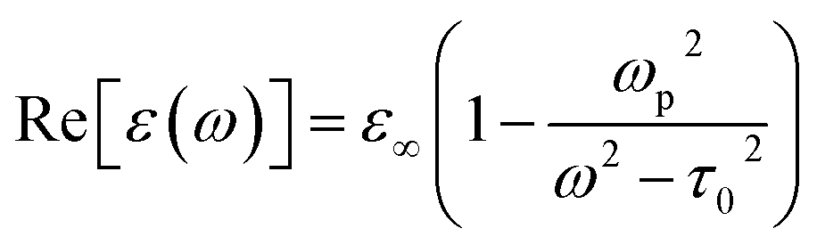 | (12) |
where ε∞ is the dielectric constant at infinitely high frequencies, τ0 is the collision frequency of electrons with ions and impurities in the structure. Taking into account that τ0 ≪ ω, the plasmon frequency can be determined at Re(ε(ω)) ≈ 0. It can also be seen that for the case of ω < ωp the real part of the expression will be negative (Re[ε(ω)] < 0). In addition, if ω is not small, Im[ε(ω)] will have small values. These two conclusions – the real part of the dielectric function is negative and has a relatively large magnitude and the imaginary part is small – are the main conditions of plasmonic resonance at a certain frequency to occur in bulk materials.
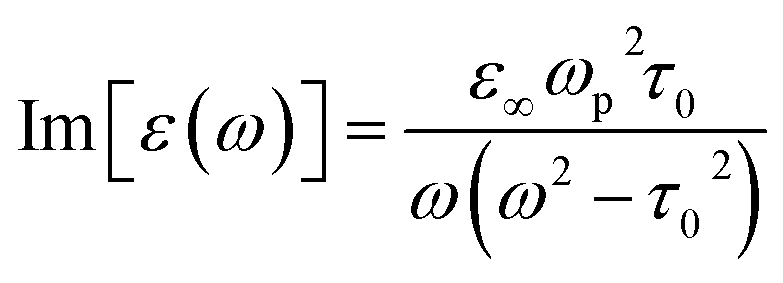
Analysis of the wavelength dependence of the real and imaginary parts of the dielectric function for different metals480 shows that the real part of their dielectric function is negative in the Vis-NIR region. In the visible region aluminum has the highest absolute value, being close to 30 at 400 nm and increasing rapidly with the wavelength. It is followed by a group of three metals behaving very similarly – silver, gold, and copper. Their values are small up to 600 nm but increase afterwards. This group is followed by palladium, platinum, and lithium, having noticeable values in the red and near infrared wavelength regions.480 In terms of the imaginary part of the dielectric function, silver has the smallest value in the visible region. It is around 0.6 at 400 nm and increases nearly linearly to 1.7 at 800 nm. Slightly higher values can be seen for lithium with similar wavelength dependence. Gold and copper are >5 at 400 nm, but then they decrease and get close to silver at 650 nm, from where the three follow the same trend. From the above it can be concluded that copper, gold, and silver are the materials with most favorable dielectric properties for efficient plasmon resonance. And indeed, silver and gold are the most widespread plasmonic materials used in SPR, SERS and other spectroscopic techniques nowadays.
The plasmonic conditions set for the real and imaginary parts of the dielectric function can be combined into the so-called quality factor as:
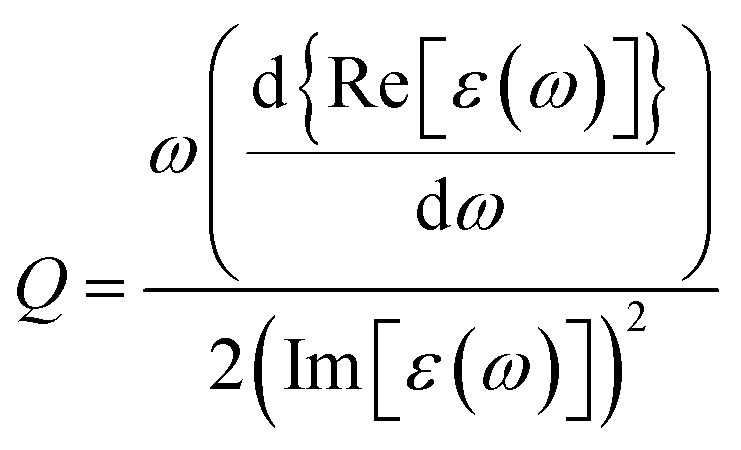 | (13) |
From eqn (13) it can be seen that the higher the rate of the change of the real part and the smaller the imaginary part of the dielectric function with frequency, the higher the quality factor is and the better the given material for plasmonic applications in the given wavelength region.
As eqn (11) shows, the excitation of SPP depends on the properties of both the metal layer and its environment. This relationship makes the excitation of surface plasmon resonance an outstanding tool for sensing, in which the changes in the dielectric properties of the local environment of the metal layer can be detected by measuring change in the resonance frequency (or the coupling angle) of surface plasmon polaritons. This is the basis of the SPR technique.
The ωSPR SPP resonance frequency is determined by the plasmon frequency of the metal and the dielectric properties of the surrounding medium:478
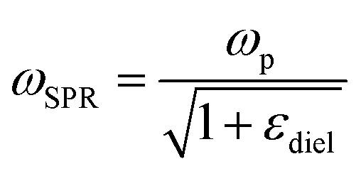 | (14) |
The local electromagnetic field resulting from the charge oscillations during SPR extends a few hundreds of nanometers from the metal surface. So, if the local environment changes within this distance, the dielectric constant will differ, and the SPR frequency will shift. The narrow resonant line shape and high angular specificity of SPR allow excellent signal-to-noise ratio and figure of merit to be obtained for SPR-based sensors, but the measurement requires inpractically strict conditions and complex geometries.478
The strict conditions are not required when surface plasmons are excited in metal NPs instead of thin layers. In this case, if the NP size is below the wavelength of the incident light, the electric field will be constant across the NP, inducing a uniform displacement of the electron density and a strong restoring force from the positive ionic core background.481 This interaction leads to collective oscillation of the free electron cloud of the NP with a characteristic oscillation resonance frequency. This phenomenon is known as localized surface plasmon resonance, or LSPR. There is no angular requirement in LSPR excitation, since the additional momentum is provided by the geometry of the NPs.481 Therefore, the change in the LSPR wavelength can be detected without gratings or prisms, by using a simple spectrometer.
Similarly to SPR, the resonance frequency of LSPR also depends on the plasmon frequency of the metal and the dielectric function of the local environment of the NP:474
 | (15) |
The main difference between ωSPR and ωLSPR is the factor 2 in the nominator, resulting in different resonance frequencies for the same metal–dielectric combinations. However, there are several advantages related to the use of quasi zero-dimensional NPs instead of two-dimensional thin layers for LSPR.474 The confined electron oscillations in LSPR cause intense local electromagnetic fields, which can be several orders of magnitude stronger than the incident field. This phenomenon is behind the concept of, for example, surface-enhanced Raman scattering. This field will be more concentrated around the edges in NPs with sharp edges, further increasing the local field intensity. It has been shown that the LSPR peak position is affected also by the size of the NPs.474 In general, the larger the particles, the more red-shifted the LSPR wavelength will be,474,482 which can be leveraged for fine-tuning the plasmonic properties of NPs. Specific NPs with asymmetric shape (e.g. nanorods) have two LSPR peaks corresponding to their longitudinal and transversal oscillation modes,483 and their separation can be tailored by the diameter and the size aspect ratio. Also, the electromagnetic field in LSPR decays in a few tens of nanometers and it is more sensitive to changes in the distance from the surface of the metal.474,478 Another specific feature of NP-based LSPR is the coupling of local fields when the NPs are brought within the local field decay length.478 This coupling can enhance the local field intensity and shift the LSPR peak position due to hybridization of modes.474
4.3. Methodology and applications
Localized surface plasmons and plasmonic enhancement are used in many spectroscopic techniques nowadays. The simplest, yet highly efficient method is LSPR, in which metallic NPs are used as sensor transducers, the plasmon resonance frequency of which shifts when the dielectric properties of their local environment change. SERS and SEF utilize the resonant amplification of the electromagnetic field of the incident or emitted light through their interaction with strongly confined plasmons of NPs. In addition to LSPR, other effects also contribute to SEF, NELIBS and NE-LA-ICPMS. The following paragraphs summarize the main principles and some of the applications of these methods.LSPR utilizes the same phenomenon, but on the boundaries of metallic NPs and their surrounding medium. Changes in the local environment are detected through the shift of the LSPR maximum wavelength of the broadband light transmitted through or reflected from the medium with NPs. The resonant frequency of NPs depends on their composition, size, geometry, dielectric environment, and separation distance.484,485 Since many LSPR methods involve ensembles of nanoparticles that have some size distribution, the measured spectral signals are averaged quantities and can exhibit heterogeneous broadening.
In contrast to SPR, LSPR does not require complex optics. Since the conditions for resonance are simpler than those of SPR, the LSPR instrumentation can consist of a white light source and a spectrometer. Optical fibers can be used to couple the incident and transmitted/reflected light to/from the metallic NPs, making the LSPR experiments and development of LSPR systems extremely flexible and allowing to perform remote measurements as well. LSPR sensors have a greater potential for miniaturization and portability and are simple to integrate with microfluidics.486
Mostly Au, Ag and Cu NPs are used in LSPR applications. These metal NPs exhibit shape and size dependent LSPR absorption and scattering bands, which is utilized to construct plasmonic sensors. They can be used as LSPR sensor transducers in three main configurations: in free-standing colloidal (homogeneous), surface-confined (heterogeneous) single NP and surface-confined (heterogeneous) NP array forms.486
There are two types of NP-based plasmonic interactions causing LSPR peak shift.474 In the first type the LSPR wavelength shifts when an analyte binds to the NPs surface and changes the local refractive index, while in the second, the plasmonic fields of several nanoparticles are coupled when an analyte brings them into proximity (aggregation), causing a remarkable shift of the LSPR wavelength and thereby a color change.474 The local field enhancement can reach a factor of 104–106 with separated metal NPs, while for colloidal aggregates487 it can be as high as 1014. Because of their large enhancement factors, colloidal aggregated NPs have been used in a variety of plasmonic applications including solar energy conversion, photocatalysis, nanomedicine, biological sensing, etc.487
Applications of LSPR for sensing cover many areas of modern technology, including gas and pH sensing, biology, medical diagnostics, or environmental protection. Several excellent review papers are available covering different fields of LSPR applications, including chemical analysis481 and especially biosensing.481,486,488–491 While most of the NP-based LSPR sensors operate in liquid environment, there are developments targeting gas sensing in air, including hydrogen,492,493 helium and argon,494 water vapor495 and volatile organic compounds.496 The simplest LSPR-based applications are based on the simple, fast and cheap colorimetric principle.497 Such methods have been developed for the detection of a variety of compounds, including metal ions,498 small organic molecules,499 proteins500,501 and DNA.502,503
A novel LSPR based approach is based on the combination of plasmonic nanostructures with other sensing methods, such as responsive photonic crystals (PCs)233,504–506 or metal oxide films.507,508 PCs are optical materials consisting of periodically arranged materials with different dielectric constants. These structures can be used as sensing materials since their diffraction wavelengths or intensities will change when they are exposed to physical or chemical stimuli.233 PCs are widely used in detection of ions509 and gases,510 and also of electric511 and magnetic fields.512 Their response can be enhanced by plasmonic NPs,233,505 and that, in addition to the amplification of the signal coming from the PC, can also be used to immobilize the recognition element, providing specificity to the sensor. Combination of opal PCs with SiO2–Au NPs resulted in three orders of magnitude increase in the limit of detection of the PC has been observed after combining it with the plasmonic gold nanoparticles.233 The capabilities of this sensing platform were demonstrated with atrazine analogues, demonstrating a sensitivity of 10–12 g mL−1.
The sensitivity of gas sensing metal oxide films was also improved by combination with plasmonic NPs. Au:CuO composites were used to develop a high-resolution LSPR spectroscopy system for the detection of pure Ar, N2, O2 gases.508 The composite structure was produced by sputtering a copper target with gold pellets on its surface, followed by a heat treatment promoting Au NP formation. A surface plasma treatment was used to activate the film for the detection of gas molecules. A one order of magnitude increase of the sensitivity was achieved, compared to the performance of copper oxide without the NPs.508
An emerging field of LSPR application is the sensing in the near-infrared (NIR) region, especially in at the wavelengths used in telecommunications (1530–1625 nm). Combination of the cheap and mature optical fiber technology with chemical and biological LSPR sensing leads to numerous new applications, especially in remote sensing technologies. As it has been discussed earlier, the metals useful for plasmonics must have a negative and high magnitude real and a small imaginary dielectric function, implying a large Q-factor. Au and Cu are the only metals meeting these criteria in the NIR region and indeed, NPs prepared from these materials showed strong absorption peaks there.513 Wide-bandgap semiconductors, like tin doled indium oxide, aluminum doped zinc oxide or titanium oxide514–516 and transition-metal oxides (molybdenum oxide,517 tungsten oxide,518 vanadium oxide519) were also found to be good candidates for NIR plasmonics. Composite NPs of gold and molybdenum oxide were used for the detection of hydrogen.517 These NPs showed strong LSPR absorption in the NIR, being responsive to hydrogen, the presence of which caused increase and shift of the plasmonic peak.517
A new method for tuning the LSPR properties can be achieved by fabricating magnetic LSPR NPs and nanostructures, allowing to change the optical properties by the application of a magnetic field, as well as to modulate the magnetic properties under irradiation at the plasmon resonance.520 NPs with combined magnetic and LSPR properties were synthesized first from bimetallic structures such as Ni–Au521 or Co–Au,522 however, the performance was found to be strongly dependent on the dimensions, shape and positioning of the different components, making the reproducible preparation a main issue.520 Recently, arrays of periodically placed cobalt NPs were found to have plasmonic properties and a quality factor comparable to that of Au NPs.520 Particle size, shape and the interparticle distance were found to have a significant impact on the optical response here as well, however, the use of an intrinsically magnetic, single metal structure makes their control remarkably easier. The LSPR absorption peak of Co NP arrays extends above the visible region making them promising for NIR LSPR applications.
Besides resonant Raman scattering, surface enhanced Raman scattering (SERS) is another phenomenon causing the enhancement of the Raman signal. SERS was first discovered in the 1970s by recording an unexpectedly large Raman signal when measuring pyridine adsorbed on a roughened silver electrode.464 The first explanations were attributing this phenomenon to the formation of strong electrochemical electromagnetic fields or molecular–metal complexes on the metal surface,524,525 as well as to the characteristics of the nanostructured metal surface and the optical excitation of the collective oscillation of electrons.526,527 The research and especially applications of SERS started to emerge in the 1990s, when, thanks to the development of compact coherent light sources and spectroscopic instrumentation, Raman spectrometers appeared in more and more spectroscopic and analytical chemistry laboratories. SERS was found to offer simple, rapid, non-invasive, and non-destructive analytical capability providing information about the bonding configuration of target molecules.528 Its proven ability for single-molecule detection drives the development of different SERS enhancement platforms for the detection of molecules on a sub-ppb or even lower levels.529 As the SERS spectrum of water is rather weak,530 SERS can efficiently be used to study biological samples and to detect biomolecules even at very low concentrations.531 SERS amplification was also observed with dielectrics and semiconductors, but with a much smaller enhancement than with metal based plasmonic structures.532
While the SERS enhancement mechanism is not completely understood yet, it is generally accepted that there are two enhancement mechanisms contributing to SERS: the so-called electromagnetic480,533 and the chemical enhancement.534 The former is based on the interaction of the incident and/or scattered light with localized surface plasmons, resulting in amplification of their electromagnetic field and the Raman scattering on molecules being in close vicinity of the plasmonic surface. This mechanism can provide SERS enhancement on the level of 6–9 orders of magnitude.535 Chemical enhancement is the result of complex formation between the plasmonic surface and the molecule, sometimes accompanied by generation of new electron energy levels, involved in resonant Raman scattering. In this regard chemical enhancement is not a plasmonic process but rather a specific Raman scattering in which the energy difference of the newly created energy levels is equal to the energy of the exciting photons. A 2–4 orders of magnitude of SERS enhancement can be attributed to this mechanism.535
The electromagnetic SERS enhancement is independent of the type of the molecule, but strongly depends on the properties of the plasmonic surface, including its material, size, shape and, in case of SERS substrates, surface roughness.536 Since Raman scattering involves photons of two different wavelengths, the electromagnetic enhancement has two distinct contributions. The first is the near-field enhancement, during which the LSPR excitation induces strong spatial localization and amplification of the excitation laser light in small spatial regions, called hotspots.536 Around the hotspots the molecules experience a much stronger electromagnetic field than in the normal laser radiation, resulting in high levels of Raman enhancement. The second is the re-radiation enhancement related to the amplification of the Raman scattered light radiated by the molecule, that arises from the environment-dependent emission by the Raman scattering molecule, as a dipole, affected by the interface of the plasmonic surface, sometimes referred as modified spontaneous emission.536 While a dipole (molecule) has a typical, symmetric emission pattern in vacuum or homogeneous medium, its irradiated electromagnetic field will be scattered at nearby interfaces and will be partly back-scattered to the dipole. This back-scattered radiation (or self-reaction field) will influence the way in which the dipole radiates power and could contribute to the enhancement of Raman scattering.536
The chemical SERS enhancement is related to the adsorption of the molecule on the plasmonic surface, accompanied by bond formation. This could contribute to the increased SRS signal in two different ways. During the resonant charge transfer the interaction between the molecule and the metal results in the creation of a metal–molecule charge transfer state, involved in resonant Raman scattering process, resulting in remarkably enhanced Raman intensity.536 In the non-resonant chemical effect, there are no new electronic states involving the resonant process, but the interaction induces changes in the geometry and electronic structure of the molecule, affecting the probability of certain Raman transitions and resulting in enhanced Raman intensities, but also slight modification of the Raman peak positions.536
From the practical point of view, SERS requires the same instrumentation as normal Raman spectroscopy. This means a narrow band coherent light source, an optical system delivering the excitation beam to the sample and the collected scattered light to the spectrometer, a notch or a steep edge filter stopping the light at the excitation wavelength to enter the spectrometer, a high-resolution spectrometer, and a sensitive detector.523 For a given SERS application the excitation wavelength can be selected based on the properties of the SERS agent or the sample. Here, LSPR wavelength and width must be considered, as well as the optical absorption and emission properties of the analyte(s) (to exploit the benefits of resonant Raman scattering (if applicable)) and avoid the overlapping of the Raman bands by fluorescence. The possibility of the damage of the sample at a given laser wavelength should be considered as well.523
Metallic NPs and colloidal systems based on them are among the most studied platforms for SERS applications. The SERS efficiency of metallic NPs, especially of Au, Ag and Cu, were early recognized and investigated by SERS researchers. Similarly to LSPR, the SERS characteristics of a colloidal system also depend on the NPs shape, size, and aggregation state.537 The aggregation of NPs in the colloid leads to increased SERS, however, if aggregation is performed without control, spatial, time and sample-to-sample variations might occur.537 The positive effect of the aggregation on SERS efficiency is related to the formation of hotspots – nanosized gaps between the NPs, in which the plasmonic fields of the neighbor particles are coupled, resulting in remarkable increase of the Raman intensity.537 Fabrication of SERS platform with large number of hotspots is the aim of many developments.
The investigation of the effect of the gold NPs shape on the SERS enhancement showed that nanorods have a larger enhancement than nanospheres, but nanostars perform even better, which can be attributed to the highly concentrated electromagnetic field at the tips.538
When using metal NPs for plasmonics, SERS can be combined with LSPR for molecular identification purposes.539,540 In fact, SERS and LSPR involve some common mechanism, namely the electromagnetic enhancement or the interaction of localized surface plasmons with the electromagnetic field of incident light. This interaction of the metallic NP with light leads to the creation of a local field around it which is proportional to the incident excitation.540 Once a molecule is in the vicinity of such a nanoparticle, it will be involved in a SERS process, but will also contribute to the shift of the LSPR wavelength due to its effect on the dielectric properties of the vicinity of the NP.540 This allows to perform SERS and LSPR measurements simultaneously.
A huge number of applications have been developed for SERS, including biology, medical diagnostics, trace element analysis, study of different gas, liquid and solid samples, from macroscopic sizes to and nanostructures. The local character and small SERS active region of plasmonic NPs can be used to study the surface of solid surfaces. For example, functional groups from grain boundaries of nanocrystalline diamond films can be enhanced selectively by dripping a drying gold NPs from a colloid onto the layer surface (Fig. 8). Sharp peaks appear in the SERS spectrum on top of the otherwise broad bands arising from the amorphous carbon intergrain phase.
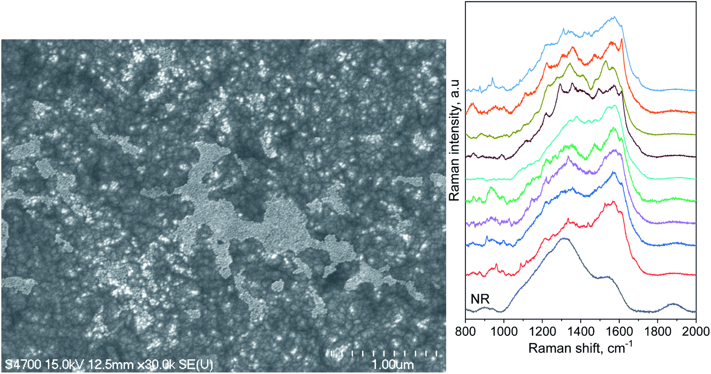 | ||
| Fig. 8 (Left) Aggregated 20 nm sized gold NPs on the surface of a nanocrystalline diamond film having 25 nm average grain size and (right) normal Raman and SERS spectra recorded on this nanodiamond layer sample (based on the authors' own data). | ||
The capabilities of SERS can be increased by combining different SERS architectures. Efficient hotspots formation has been demonstrated between two or several NPs, as well as between a flat metallic surface and the curved surface of a gold NP.541,542 An even better gain can be achieved by combining a periodic SERS array with NPs. A giant SERS and SEF enhancement has been observed in structures consisting of nanometer sized gold particles trapped in gold coated inverse pyramids fabricated in silicon by photolithographic technique543 (Fig. 9). The enhancement was found to increase with increasing the NP size from 50 to 200 nm, which was related to the shift of the contact point of the nanosphere and the pyramid surface towards the region with highest near-field enhancement of the pyramid.
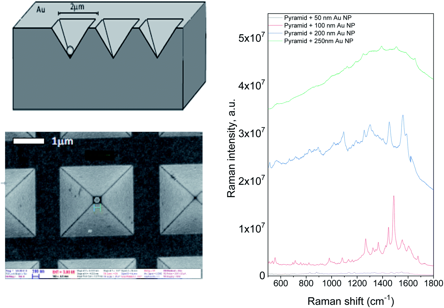 | ||
| Fig. 9 (Top left) Schematic representation of the Au NP trapped in gold coated void of inverse pyramid shape, prepared in a silicon substrate (bottom left) SEM image of the fabricated structure (from the top) with a gold NP clearly visible inside the void and (right) SERS enhancement obtained with the inverse pyramid containing NPs of different size between 50 and 250 nm (based on the authors' own data). | ||
Novel methods have been developed for cost-efficient SERS substrate fabrication for different applications. Self-assembly of metallic NPs at water–oil interface was found to be a convenient and efficient route to obtain densely packed plasmonic nanoparticles which have small interparticle distances.544 In this case, the surface charge preventing aggregation and self-assembly can be removed by using chemical modifiers on the NP surface, addition of co-solvents or charge screening by promoters, or their combination.544 After the fabrication the liquid plasmonic arrays are usually transformed into free-standing solid films. The capabilities of such 2D arrays and fabrication method were demonstrated with DNA,545 microRNA,546 multiplex analyte detection547 and others. A simple, one-step gas phase technique was used to prepare structures with tunable plasmonic enhancement utilizing spark discharge nanoparticle generation and deposition of the NPs onto glass microfiber filters.31 The Au/Ag binary NPs obtained by this method showed remarkable signal enhancement be achieved over a large surface area, and the plasmonic properties of the SERS substrate were easily tunable by changing the composition of the NPs.
The NELIBS technique has been first demonstrated on plant leaves using low-energy LIBS.469 Colloidal silver NPs were applied to the leaf surface resulting in 3–5 times enhancement of the LIBS intensity of the fresh leaf sample. NELIBS was found to be even more efficient when placing NPs on conducting (metallic) surfaces,551 while less amplification was observed in case of insulators.552 Therefore, metal samples are mostly used in NELIBS studies, but the method was also used on transparent materials,552,553 gemstones,553 solutions,554,555 fruits and vegetables,556 food557,558 and biological tissues.469 Among these studies, the enhancement factors have shown big variations, ranging from a factor of a few to several orders of magnitude. It was shown, that the material and surface concentration of NPs, as well as the laser wavelength and irradiance all have a great impact on the signal enhancement achievable.12,550
The production of the plasma plays a crucial role in LIBS. In general, the plasma induction needs the production of free electrons, the so-called seed electrons.559 In case of solids, after vaporization and ionization of the sample this starts with multiphoton ionization, during which electrons collect the energy of multiple photons so that the total absorbed energy is enough to overcome the work function of the solid or the ionization energy of the laser vaporized atoms.559 When metal NPs are placed on the sample, the induced LSPR can enhance the electromagnetic field of the incident radiation, and this can change the way the ablation and the plasma induction occur: the laser–sample interaction will mainly be mediated by the NPs.559
According to recent studies, different mechanisms occur when metal NPs are used for LIBS in conductive and insulator samples. When NPs are deposited on a metallic surface, the LSPR enhancement of the laser field changes production of seed electrons from typical multiphoton ionization to field emission, resulting in instantaneous emission of electrons before the particles are completely deteriorated upon the effect of the laser.551 In addition, electrons accelerated upon laser irradiation provide additional electron flow that contributes to induction of an efficient breakdown and an efficient plasma excitation.559 Since field enhancement is produced on several NP hotspots simultaneously, several electron extraction points are available in the laser spot, leading to multiple ignition points of the plasma.559
When NPs are placed on an insulator sample, the LSPR enhancement is too weak to remove electrons from the bulk substrate.551 In this case, depending on the laser irradiance and excitation wavelength, two mechanism can occur. If laser is in resonance with the localized surface plasmons, the electromagnetic field enhancement due to NPs surface electron oscillations will cause strong local heating on the sample surface by the NPs.551 This can be accompanied by optical breakdown of NPs and generation of the plasma and this can extend to the sample in the close vicinity of NPs, if the irradiance is high enough.551 If the laser pulse is off-resonance with surface plasmons and the interparticle distance between NPs is small, electron transfer and charge unbalancing can occur that can initiate optical breakdown of the NPs.551
In case of semiconductors, depending on the band gap energy of the sample, NELIBS works like with metallic or dielectric samples.559 Typical examples are amorphous silicon and doped silicon. The first is a material with relatively large band gap and NELIBS does not produce any noticeable enhancement on Si emission with that, while in the additional electron energy levels introduced by doping allow to obtain 10 times enhancement of the LIBS signal.559
The issue of sample contamination after NELIBS measurement was also investigated. In ref. 552, it was found that the elements coming from NPs ablation constitute 0.004% of the total ablated material. In most cases NPs are almost completely removed from the sample after one laser shot and after three laser shots the sample is completely free from the NPs contamination.559
The application potential of NELIBS has been demonstrated on many different samples, ranging from metals to liquids. The highly efficient enhancement obtained on conducting surfaces and allowing the detection of trace elements to sub-ppm level put the analysis of metallic samples to the front of NELIBS research.552 The capabilities of the method were tested with titanium alloys and brass560 and other metals.561 A promising application of NELIBS is the measurement of liquid phase samples, which is based on the mechanism of NELIBS characteristic for insulators.
As it has been described earlier, the irradiation of metal NPs placed on insulator substrate with the laser pulse will initiate breakdown of the nanoparticles and plasma generation, and this plasma can include analytes being in close vicinity of those NPs.551 This can be attempted by dripping and drying the sample onto the NPs attached to a substrate. This approach was used to enhance the copper signal by delivering the sample to NPs from liquid solution.554 A sub-ppb detection limit was achieved for silver in a solution of silver nitrate.550 Modified SERS substrates consisting of Ag NPs on indium-tin-oxide glass were also used for quantitative NELIBS measurements on liquid solutions of Mn, Zn and Cr, and it was found that interparticle distance plays crucial role in efficient enhancement.12
A biological sample was used as subject in the first demonstration of the NELIBS effect. A colloidal silver solution was applied to a leaf surface469 allowing the measurements of several alkaline metals with an enhancement of about a factor of 5. This method was used to study other biological systems as well. Different types of animal fodder (artificial feed, barley, and clover) and ancient and contemporary bones were analyzed, in order to correlate their elemental composition and determine the differences between feeding of animals over time.558 Sprinkling biosynthesized silver NPs were deposited onto the bovine bone and fodder sample surface before analysis and the obtained NELIBS data were analyzed by statistical and direct evaluation. Proteins in canned tuna fish were also assessed using NELIBS technique, and the method was found to be promising for production monitoring of canned foods containing proteins. For this study biosynthesized silver NPs were used to enhance the LIBS emission intensity of fish samples.557 Another study focused on the detection of trace pesticides and heavy metal residues in fruits and vegetables. Compared to standard LIBS, NELIBS gave two orders of magnitude lower detection limit for these contaminants and allowed to perform mapping measurements on vegetable leaves.556
Laser Ablation Inductively Coupled Plasma Mass Spectrometry (LA-ICPMS) is another highly sensitive and fast analytical technique, allowing to perform elemental analysis on solid samples by ablating their surface and determining the composition of the formed particulate material via mass spectrometry.562 It requires little or no sample preparation, the analysis can be performed on conducting, non-conducting, opaque and transparent materials; and allows to perform bulk analysis, depth profiling or elemental/isotope mapping.562
While the operating principle of LIBS and LA-ICPMS are different, they are common in the way of the excitation of the sample to be measured.562 The sample is illuminated with an intense laser pulse that ablates its surface. The generated plasma is detected by LIBS, while the particles are transported to the ICP torch and from there into the mass spectrometer. So, it can be expected that the NP enhancement working for LIBS should improve the performance of LA-ICPMS as well. This has been demonstrated first on conductive samples by achieving an enhancement of two orders of magnitude.40 The sample preparation was like in case of NELIBS: gold and silver NPs were dried onto the sample surface. The successful demonstration of NE-LAICPMS on conductive materials was accompanied with measurement on insulating ceramic and glass samples, however, no enhancement has been observed for the latter.40 Later it was shown that the effect works for metallic elements in both conductive and dielectric matrices.562 The NE-LAICPMS enhancement was found to be dependent on both the typology, concentration and size of the dropped nanoparticles and the composition of the sample, and different elements showed different enhancement in the same matrix, just as the same element showed different enhancement in different matrices.562 Study of the effect of NPs on the aerosol formed during laser ablation showed that the highest number of particles was generated using the smallest (10 nm) particles, and, in contrast to normal LA-ICPMS, where the number of particles increased in proportion to the used fluence, the aerosol generation efficiency showed a maximum for NE-LAICPMS at moderate laser powers.
The origin of this behavior was attributed to two reasons.563 The first is related to the plasmonic properties of NPs, similarly to LIBS: the gaps between close NPs work as ignition points of plasma, and in this way whole plasma dynamics changed. This results in the formation of smaller particles at the expense of larger ones resulting in more efficient transport, evaporation and ionization in ICP. The second is the change of the optical properties of the surface due to the presence of NPs, increasing the energy transfer of the laser and the efficiency of the ablation of the sample, and thus leading to higher mass production.563
The mechanism of SEF is not precisely determined yet. The main reason is most probably the presence of different interactions between the fluorophore (analyte) and the metallic surface. SEF is supposed to be a complex phenomenon involving surface plasmons and optical near-fields, enhancing the fluorescence intensity and photostability, but also affecting its lifetime.565 The electromagnetic interactions involved in SEF can be divided into three categories: LSPR, non-radiative energy transfer, and intrinsic radiative decay.418 Some of these coupling interactions are related to the spectral overlap between surface plasmons and the emission band of the analyte, and each of them dominates SEF on different separation distances between the fluorophore and the metallic NP.566,567
Localized surface plasmon resonance influences SEF through the increase of the excitation rate, by enhancing the local electromagnetic field. This effect is similar to the electromagnetic enhancement of SERS. It is supposed that the LSPR generated on metallic NPs modifies the absorption characteristics of the fluorophores by increasing their cross-section,568 which amplifies the fluorescence intensity by coupling with the NPs.454 The geometry of the NPs plays crucial role is this interaction, since due to the field effect, SEF enhancement will be stronger at the edges and corners of NPs of complex size,569,570 but the NP size and shape affect the LSPR conditions (maximum wavelength and spectral width) as well.
The non-radiative interaction mediates the surface plasmons' interaction with the fluorophore.418 The character of this effect determines whether quenching or enhancement of the fluorescence will occur:571 the energy transfer between the surface plasmons and the analyte will increase the fluorescence intensity only in some distance between the analyte and the metallic surface. According to recent studies, the fluorescence enhancement achieved within the distance of up to 10–15 nm from the metallic surface can be explained through the Forster resonance energy transfer (FRET)572 (or non-radiative dipole–dipole coupling), decaying rapidly with distance. For larger separations (10–50 nm) SEF can be explained through the role the NP characteristics play in light coupling (the so-called Purcell effect).564 It was shown that at such distances the enhancement is higher on metallic structures absorbing light rather than scattering it, as well as on NPs having concentrated and confined electromagnetic fields around sharp edges or narrow gaps.573
The role of intrinsic radiative decay is also more remarkable for the case when the analytes and the NPs are in close vicinity of each other. In this case the fluorophore is coupled to surface plasmons of NP generating new SEF decay pathways for energy transfer. The analytes are excited by the non-radiative energy transfer from NPs and transmit this energy to the far-field through radiative transfer, resulting in enhanced fluorescence intensity.567 The rate of the energy transfer can be controlled by fine-tuning the metallic structures, which, due to the enhanced rate of radiative decay, will further decrease the fluorescence lifetime of the fluorophore.567
As it can be expected, SEF is strongly affected by characteristics of the metallic NPs. The type of metal determines the useful plasmonic wavelength region, which is further narrowed by the particles' size and shape. The NPs size is also related to the SEF specific “scattering to absorption ratio” affecting the non-radiative interaction (interestingly, the latter was found to be independent of the aspect ratio for SEF574). In general, absorption is dominant for NPs smaller than 20 nm, and scattering occurs for larger sizes and further increases with the size of the particles. Shape plays a remarkable role in determining the spectral properties of NPs:574 elongated and complex forms can be used to fabricate structures with dual LSPR peaks and specific hotspot regions, where the electromagnetic field enhancement by LSPR can be concentrated.575 A summary of various nanostructures and NPs with different shapes and geometries, and their experimentally determined SEF enhancement factors are provided in ref. 567. It can also be concluded from there that, in addition to shape, the enhancement of metallic NPs critically depends also on their interparticle distance, dielectric constant, and physical dimensions.
Since surface enhanced fluorescence emission is quenched if the analyte is in close vicinity of the surface of NPs, the most important and critical criterion for efficient SEF is to fabricate a layer of non-metallic material on the NP surface, referred to as a spacer.576,577 A large variety of spacers have been reported that, based on the materials used for distance modulation, can primarily be divided into three categories: inorganic (e.g., silica), organic (e.g., polymer, proteins, DNA, and others) and hybrid spacers.578 In case of metallic NPs, the spacer on the surface of the particle is obtained by fabrication of core–shell structures. These structures are defined as consisting of an inner isolated NP coated with one or several shell layers, or as inverse core–shell systems with the fluorophore encapsulated into a hollow core metallic NP.
Preparation of core–shell SEF NPs requires multiple steps.579 The first step is the fabrication of the nanoparticles; this can be done using different metals (gold, silver, copper, zinc, alloy580), obtaining nanoobjects of various size and shape, including rods, triangles, cubes, stars.581 In this step, the plasmonic properties of the metallic core can be engineered according to the requirements of the particular SEF application. After their fabrication, the metallic NPs should be stabilized against agglomeration by the formation of an appropriate surface layer. Here particular attention should be paid not to affect their unique optical properties. This can be achieved by using molecular layers, or even thick coatings that could serve as base layer of the spacer.579 When selecting the stabilizer, in addition to its dielectric characteristics, the compatibility with the spacer material must also be taken into account. The third, crucial step, having significant impact on the efficiency of the SEF agent is the fabrication of the spacer itself. This is followed by functionalization of the silica surface and the attachment of the fluorophore through electrostatic attraction or covalent binding.578 Various kinds of fluorophores have been assembled onto the silver–silica and gold–silica core–shell NPs,582,583 providing SEF with enhancement factors ranging from 2 to 20.
Since the role of the spacer is to provide elevation for the analyte from the quenching zone to the SEF distance, spacers must be of uniform and precisely engineered thickness, which is not so easy to control on the nanoscale.579 The simplest method for this is the layer-by-layer deposition of polymer, dielectric or hybrid composite spacers. It was found that multi-layered films with hybrid nanocomposites deliver much higher intensity SEF.579,584,585 Various materials such as polyelectrolytes were used as building blocks to fabricate functional multi-layered thin films for SEF, composed of sequentially stacked functional materials such as DNA probes or small nanoparticles586 and the fluorophores positioned to the last layer. The multilayer approach can be used to obtain stimuli-responsive structures by incorporating materials being sensitive to temperature, pH, light, etc. that can be used to control the properties of SEF agents.579,587
In colloidal NP systems the enhancement factors in suspensions were found to be up to several orders of magnitude. In the first studies silver core and silica shell particles were used in a solution sensing platform.583 These monodisperse structures were called as metal-enhanced fluorescence nanoballs, the performance of which was demonstrated for potential applications in cellular imaging and solution-based sensing by incorporating near-infrared emitting probes within the silica shell.583 Due to its chemical inertness, good optical transparency, biocompatibility, and low toxicity588,589 silica is amongst the most widely used inorganic spacer materials in colloidal systems. Another advantage of silica spacers is the possibility to obtain uniform thickness up to 90 nm by controlling only the silica precursor concentration during the fabrication process.590 In addition, the surface of silica could easily be modified with different functional groups, enabling simple conjugation of fluorophores and biomolecules.
Beside metallic core and dielectric shell NP configurations, silica-based hybrid nanocomposite spacer systems can be used in form of dye-silica inner beads decorated with metal NPs or surrounded by a continuous thin metal shell.591 Having a favorable cavity size, the emission properties of the fluorophore can be enhanced significantly in such structures, which can be explained by two effects: the LSPR enhancement of the exciting electromagnetic field within the cavity, and the reduction of the fluorescence lifetime due to the strong near-field interaction between the fluorophore and cavity.592 Further advantages of such nanostructures include the tunability of the LSPR wavelength by controlling the core to shell ratio,593 the standardization of surface functionalization: the same metallic shell can be used with a broad variety of fluorophores578 and the possibility to combine SEF with SERS.582 The general fabrication procedure of inverse core–shell structures consists of coating the fluorophore with silica of the required thickness, followed by surface functionalization of the outside silica surface and the preparation of the metallic shell in form of continuous film or a layer of small metallic NPs.578
SEF has numerous applications in various fields of chemical analysis and especially of biosensing and medical diagnostics. A number of review papers were published on this topic in the past few years454,579,594–596 indicating the versatility of applications and the rapid development of SEF.
5. Conclusions
In the present review, we attempt to provide the reader with a comprehensive overview of the progress in the field of nanoparticle-related laser and plasma spectroscopy research. We believe that the results disseminated recently in the literature properly illustrate the symbiotic connection between materials science and analytical laser/plasma spectroscopy. This connection is not one-directional, but there are multiple ways through which these research areas can benefit from each other and thereby enjoy a mutually supportive relationship. As we have shown, modern laser and plasma spectroscopy technologies offer versatile and effective methods for nanoparticle characterization and monitoring nanoparticle synthesis, thereby also contributing to the understanding of nanoparticle formation mechanisms. At the same time, materials science can boost the performance of laser and plasma spectroscopy by providing suitable and tunable nanoparticles useful for plasmonic analytical signal enhancement. Based on the rate of progress in the past decades, it can be expected that this relationship will flourish in the future as well. As an example, interesting recent fundamental works dealing with the directional emission of electrons and ions from isolated nanoparticles induced by femto- and attosecond laser impulses can be mentioned.597,598 The combination of nm-scale sampling on sub-fs time scales could open new analytical possibilities for the monitoring of near-field induced reaction yields on the surface of nanoparticles (“reaction nanoscopy”)599 or for the differentiation of single particles and their dimers based on their plasmonic characteristics,600 to name just a couple of options.Conflicts of interest
There are no conflicts of interest to declare.Acknowledgements
The funding received from the National Research, Development and Innovation Office of Hungary through projects K 129063, GINOP-2.3.2-15-2016-00036, EFOP-3.6.2-16-2017-00005 and VEKOP-2.3.2-16-2016-00011, and from the Ministry for Innovation and Technology of Hungary through the NKFIH-1279-2/2020 TKP 2020 program is acknowledged. One of the authors (A. Kohut) is also grateful for the support received from the ÚNKP-20-4 – New National Excellence Program of the Ministry for Innovation and Technology from the source of the National Research, Development and Innovation Fund. The open access publication of this work has been supported by the University of Szeged Open Access Fund, under Grant No. 5391.References
- A. Schmidt-Ott, Spark Ablation: Building Blocks for Nanotechnology, Jenny Stanford Publishing, Boca Raton, 1st edn, 2020 Search PubMed.
- R. Vajtai, Springer Handbook of Nanomaterials, Springer, Berlin, Heidelberg, 1st edn, 2013 Search PubMed.
- A. V. Nikam, B. L. V. Prasad and A. A. Kulkarni, CrystEngComm, 2018, 20, 5091–5107 RSC.
- L. Xu, X. Qi, X. Li, Y. Bai and H. Liu, Talanta, 2016, 146, 714–726 CrossRef CAS PubMed.
- R. Lucena, B. M. Simonet, S. Cárdenas and M. Valcárcel, J. Chromatogr. A, 2010, 1218, 620–637 CrossRef PubMed.
- J. Lei and H. Ju, Chem. Soc. Rev., 2012, 41, 2122–2134 RSC.
- P. C. Ray, Chem. Rev., 2010, 110, 5332–5365 CrossRef CAS PubMed.
- M. E. Stewart, C. R. Anderton, L. B. Thompson, J. Maria, S. K. Gray, J. A. Rogers and R. G. Nuzzo, Chem. Rev., 2008, 108, 494–521 CrossRef CAS PubMed.
- X. Jiang, K. Huang, D. Deng, H. Xia, X. Hou and Ch. Zheng, TrAC, Trends Anal. Chem., 2012, 39, 38–59 CrossRef CAS.
- J. Langer, D. J. de Aberasturi, J. Aizpurua, R. A. Alvarez-Puebla and B. Auguie, et al. , ACS Nano, 2020, 14, 28–117 CrossRef CAS PubMed.
- A. Kohut, A. Kéri, V. Horváth, J. Kopniczky, T. Ajtai, B. Hopp, G. Galbács and Z. Geretovszky, Appl. Surf. Sci., 2020, 531, 147268 CrossRef CAS.
- D. J. Palásti, P. Albrycht, P. Janovszky, K. Paszkowska, Z. Geretovszky and G. Galbács, Spectrochim. Acta, Part B, 2020, 166, 105793 CrossRef.
- S. Mourdikoudis, R. M. Pallares and N. T. K. Thanh, Nanoscale, 2018, 10, 12871–12934 RSC.
- C. Fornaguera and C. Solans, Int. J. Polym. Sci., 2018, 2018, 6387826 Search PubMed.
- A. Kohut, L. Ludvigsson, B. O. Meuller, K. Deppert, M. E. Messing, G. Galbács and Z. Geretovszky, Nanotechnology, 2017, 28, 475603 CrossRef CAS PubMed.
- B. Ferreira da Silva, S. Pérez, P. Gardinalli, R. K. Singhal, A. A. Mozeto and D. Barcelo, TrAC, Trends Anal. Chem., 2011, 30, 528–540 CrossRef CAS.
- C. M. Hussain, Handbook of Nanomaterials in Analytical Chemistry, Elsevier, Amsterdam, 1st edn, 2020 Search PubMed.
- M. Valcárcel and A. I. López-Lorente, Gold Nanoparticles in Analytical Chemistry, Comprehensive Analytical Chemistry, Elsevier, Amsterdam, 2014, vol. 66 Search PubMed.
- S. Shtykov, Nanoobjects and Nanotechnologies in Analytical Chemistry, de Gruyter, Berlin, 2018 Search PubMed.
- M. Sajid and J. Płotka-Wasylka, Microchem. J., 2020, 154, 104623 CrossRef CAS.
- M. Valcárcel, S. Cardenas and B. M. Simonet, Anal. Chem., 2007, 79, 4788–4797 CrossRef PubMed.
- F. Adams and C. Barbante, Chemical Imaging Analysis, Comprehensive Analytical Chemistry, Elsevier, Amsterdam, 2015, vol. 69 Search PubMed.
- A. S. de Dios and M. E. Díaz-García, Anal. Chim. Acta, 2010, 666, 1–22 CrossRef CAS PubMed.
- O. Axner and G. Galbács, in Encyclopedia of Analytical Chemistry, ed. R. A. Meyers, John Wiley & Sons, Hoboken, New Jersey, 2012, Laser spectrometric techniques in analytical atomic spectrometry, pp. 1–113 Search PubMed.
- J. Pareja, S. López, D. Jaramillo, D. W. Hahn and A. Molina, Appl. Opt., 2013, 52, 2470–2477 CrossRef CAS PubMed.
- O. A. Nassef and H. E. Elsayed-Ali, Spectrochim. Acta, Part B, 2005, 60, 1564–1572 CrossRef.
- Q. Lin, G. Niu, Q. Wang, Q. Yu and Y. Duan, Appl. Spectrosc. Rev., 2013, 48, 487–508 CrossRef CAS.
- M. Bonta, J. J. Gonzalez, C. Derrick Quarles, R. E. Russo, B. Hegedüs and A. Limbeck, J. Anal. At. Spectrom., 2016, 31, 252–258 RSC.
- M. Tarik, G. Lotito, J. A. Whitby, J. Koch, K. Fuhrer, M. Gonin, J. Michler, J.-L. Bolli and D. Günther, Spectrochim. Acta, Part B, 2009, 64, 262–270 CrossRef.
- I. B. Gornushkin, J. E. Kim, B. W. Smith, S. A. Baker and J. D. Winefordner, Appl. Spectrosc., 1997, 51, 1055–1059 CrossRef CAS.
- A. Kohut, A. Kéri, V. Horváth, J. Kopniczky, T. Ajtai, B. Hopp, G. Galbács and Z. Geretovszky, Appl. Surf. Sci., 2020, 531, 147268 CrossRef CAS.
- D. Zhang, B. Gökce and S. Barcikowski, Chem. Rev., 2017, 117, 3990–4103 CrossRef CAS PubMed.
- T. Amodeo, C. Dutouquet, F. Tenegal, B. Guizard, H. Maskrot, O. Le Bihan and E. Fréjafon, Spectrochim. Acta, Part B, 2008, 63, 1183–1190 CrossRef.
- P. Purohit, F. J. Fortes and J. J. Laserna, Angew. Chem., Int. Ed., 2017, 56, 1–6 CrossRef PubMed.
- P. Purohit, F. J. Fortes and J. J. Laserna, Anal. Chem., 2019, 91, 7444–7449 CrossRef CAS PubMed.
- D. Mozhayeva and C. Engelhard, J. Anal. At. Spectrom., 2020, 35, 1740–1783 RSC.
- M. D. Montano, J. W. Olesik, A. G. Barber, K. Challis and J. F. Ranville, Anal. Bioanal. Chem., 2016, 408, 5053–5074 CrossRef CAS PubMed.
- R. Xu, Particuology, 2015, 18, 11–21 CrossRef.
- M. Pintér, T. Ajtai, G. Kiss-Albert, D. Kiss, N. Utry, P. Janovszky, D. Palásti, T. Smausz, A. Kohut, B. Hopp, G. Galbács, Á. Kukovecz, Z. Kónya, G. Szabó and Z. Bozóki, Atmos. Environ., 2018, 178, 118–128 CrossRef.
- M. Holá, Z. Salajková, A. Hrdlička, P. Pořízka, K. Novotný, L. Čelko, P. Šperka, D. J. Novotný, P. Modlitbová, V. Kanický and J. Kaiser, Anal. Chem., 2018, 90, 11820–11826 CrossRef PubMed.
- M. Dell'Aglio, R. Alrifai and A. De Giacomo, Spectrochim. Acta, Part B, 2018, 148, 105–112 CrossRef.
- Z. Abdullaeva, Synthesis of Nanoparticles and Nanomaterials: Biological Approaches, Springer Nature Switzerland, Cham, 1st edn, 2017 Search PubMed.
- A. S. H. Makhlouf and A. Barhoum, Fundamentals of Nanoparticles, Elsevier, Amsterdam, 1st edn, 2018 Search PubMed.
- M. Naito, T. Yokoyama, K. Hosokawa and K. Nogi, Nanoparticle Technology Handbook, Elsevier, Amsterdam, 3rd edn, 2018 Search PubMed.
- N. G. Semaltianos, Crit. Rev. Solid State Mater. Sci., 2010, 35, 105–124 CrossRef CAS.
- T. V. Pfeiffer, J. Feng and A. Schmidt-Ott, Adv. Powder Technol., 2014, 25, 56–70 CrossRef CAS.
- P. Purohit, F. J. Fortes and J. J. Laserna, Anal. Chem., 2021, 93, 2635–2643 CrossRef CAS PubMed.
- A. Scheeline, J. A. Norris, J. C. Travis, J. R. Devoe and J. P. Walters, Spectrochim. Acta, Part B, 1981, 36, 373–383 CrossRef.
- A. Scheeline, Mikrochim. Acta, 1990, 100, 247–285 CrossRef.
- P. W. J. M. Boumans, in Analytical Emission Spectroscopy, ed. E. L. Grove, Marcel Dekker, New York, 1972 Search PubMed.
- C. A. Bye and A. Scheeline, Appl. Spectrosc., 1993, 47, 2022–2030 CrossRef CAS.
- C. Schulz, B. F. Kock, M. Hofmann, H. Michelsen, S. Will, B. Bougie, R. Suntz and G. Smallwood, Appl. Phys. B: Lasers Opt., 2006, 83, 333–354 CrossRef CAS.
- D. Mukherjee, A. Rai and M. R. Zachariah, Aerosol Sci., 2006, 37, 677–695 CrossRef CAS.
- B. K. McMillin, P. Biswas and M. R. Zachariah, J. Mater. Res., 1996, 11, 1552–1561 CrossRef CAS.
- X. Liu, M. E. Smith and S. D. Tse, Appl. Phys. B: Lasers Opt., 2010, 100, 643–653 CrossRef CAS.
- A. O'Keefe and D. A. G. Deacon, Rev. Sci. Instrum., 1988, 59, 2544–2551 CrossRef.
- I. H. Hutchinson, Principles of Plasma Diagnostics, Cambridge University Press, Cambridge, 2nd edn, 2002 Search PubMed.
- H. R. Griem, Plasma Spectroscopy, McGraw-Hill, New York, 1st edn, 1964 Search PubMed.
- H. R. Griem, Principles of Plasma Spectroscopy, Cambridge University Press, Cambridge, 1997 Search PubMed.
- H.-J. Kunze, Introduction to Plasma Spectroscopy, Springer, Berlin, Heidelberg, 1st edn, 2009 Search PubMed.
- A. R. Hanna and E. R. Fisher, J. Vac. Sci. Technol., A, 2020, 38, 020806 CrossRef CAS.
- J. A. Aguilera and C. Aragón, Spectrochim. Acta, Part B, 2008, 63, 784–792 CrossRef.
- C. A. Bye and A. Scheeline, Spectrochim. Acta, Part B, 1993, 48, 1593–1605 CrossRef.
- A. Scheeline, G. J. Kamla and M. J. Zoellner, Spectrochim. Acta, Part B, 1984, 39, 677–691 CrossRef.
- W. L. Wiese, Spectrochim. Acta, Part B, 1991, 46, 831–841 CrossRef.
- C. Yubero, M. D. Calzada and M. C. Garcia, J. Phys. Soc. Jpn., 2005, 74, 2249–2254 CrossRef CAS.
- N. Konjević and W. L. Wiese, J. Phys. Chem. Ref. Data, 1990, 19, 1307–1385 CrossRef.
- J. M. Palomares, S. Hübner, E. A. D. Carbone, N. De Vries, E. M. Van Veldhuizen, A. Sola, A. Gamero and J. J. A. M. Van Der Mullen, Spectrochim. Acta, Part B, 2012, 73, 39–47 CrossRef CAS.
- C. Aragón and J. A. Aguilera, Spectrochim. Acta, Part B, 2008, 63, 893–916 CrossRef.
- W. I. Wiese, Natl. Stand. Ref. Data Ser., 1969, 22, 306 Search PubMed.
- J. A. Aparicio, M. A. Gigosos, V. R. Gonzalez, C. Perez, M. I. de la Rosa and S. Mar, J. Phys. B: At., Mol. Opt. Phys., 1998, 31, 1029–1048 CrossRef CAS.
- W. L. Wiese and J. R. Fuhr, J. Phys. Chem. Ref. Data, 2007, 36, 1287–1345 CrossRef CAS.
- G. V. Vogman and U. Shumlak, Rev. Sci. Instrum., 2011, 82, 103504 CrossRef CAS PubMed.
- R. M. van der Horst, T. Verreycken, E. M. van Veldhuizen and P. J. Bruggeman, J. Phys. D: Appl. Phys., 2012, 45, 345201 CrossRef.
- C. Yubero, M. S. Dimitrijević, M. C. García and M. D. Calzada, Spectrochim. Acta, Part B, 2007, 62, 169–176 CrossRef.
- D. Xiao, C. Cheng, J. Shen, Y. Lan, H. Xie, X. Shu, Y. Meng, J. Li and P. K. Chu, Phys. Plasmas, 2014, 21, 053510 CrossRef.
- H. Onishi, F. Yamazaki, Y. Hakozaki, M. Takemura, A. Nezu and H. Akatsuka, Jpn. J. Appl. Phys., 2021, 60, 026002 CrossRef CAS.
- A. A. Fridman and L. A. Kennedy, Plasma Physics and Engineering, CRC Press, Boca Raton, Florida, 2nd edn, 2011 Search PubMed.
- K. Yambe and S. Satou, Phys. Plasmas, 2016, 23, 023509 CrossRef.
- T. Atwee, L. Aschke and H. J. Kunze, J. Phys. D: Appl. Phys., 2000, 33, 2263–2267 CrossRef CAS.
- F. Rezaei, Appl. Opt., 2020, 59, 3002 CrossRef CAS PubMed.
- H. Zhang, Y. Wu, H. Sun, F. Yang, M. Rong, F. Jiang, C. Wang and W. Huang, Plasma Chem. Plasma Process., 2019, 39, 1429–1447 CrossRef CAS.
- H. R. Griem, Phys. Rev., 1963, 131, 1170–1176 CrossRef.
- R. W. P. McWhirter, in Plasma Diagnostic Techniques, ed. R. H. Huddlestone and S. L. Leonard, Academic Press, New York, 1st edn, 1965, ch. 5, pp. 201–264 Search PubMed.
- A. Kohut, G. Galbács, Z. Márton and Z. Geretovszky, Plasma Sources Sci. Technol., 2017, 26, 045001 CrossRef.
- G. Cristoforetti, A. De Giacomo, M. Dell'Aglio, S. Legnaioli, E. Tognoni, V. Palleschi and N. Omenetto, Spectrochim. Acta, Part B, 2010, 65, 86–95 CrossRef.
- V. K. Unnikrishnan, K. Alti, V. B. Kartha, C. Santhosh, G. P. Gupta and B. M. Suri, Pramana, 2010, 74, 983–993 CrossRef CAS.
- H. R. Griem, Phys. Rev., 1962, 128, 997–1003 CrossRef.
- J. A. Aguilera and C. Aragón, Spectrochim. Acta, Part B, 2007, 62, 378–385 CrossRef.
- L. Sun and H. Yu, Talanta, 2009, 79, 388–395 CrossRef CAS PubMed.
- B. Praher, V. Palleschi, R. Viskup, J. Heitz and J. D. Pedarnig, Spectrochim. Acta, Part B, 2010, 65, 671–679 CrossRef.
- A. Safi, S. H. Tavassoli, G. Cristoforetti, S. Legnaioli, V. Palleschi, F. Rezaei and E. Tognoni, J. Adv. Res., 2019, 18, 1–7 CrossRef CAS PubMed.
- G. J. Bastiaans and R. A. Mangold, Spectrochim. Acta, Part B, 1985, 40, 885–892 CrossRef.
- P. Bruggeman, N. Sadeghi, D. C. Schram and V. Linss, Plasma Sources Sci. Technol., 2014, 23, 023001 CrossRef CAS.
- S. E. Pratsinis, Prog. Energy Combust. Sci., 1998, 24, 197–219 CrossRef CAS.
- H. K. Kammler, L. Mädler and S. E. Pratsinis, Chem. Eng. Technol., 2001, 24, 583–596 CrossRef CAS.
- F. Schneider, PhD thesis, University of Duisburg-Essen, 2020.
- J. Wei, Y. Ren, Y. Zhang, B. Shi and S. Li, J. Aerosol Sci., 2019, 133, 72–82 CrossRef CAS.
- F. Meierhofer, L. Mädler and U. Fritsching, AIChE J., 2020, 66, 66 CrossRef.
- T. Dreier and C. Schulz, Powder Technol., 2016, 287, 226–238 CrossRef CAS.
- C. Schulz, T. Dreier, M. Fikri and H. Wiggers, Proc. Combust. Inst., 2019, 37, 83–108 CrossRef CAS.
- I. Rahinov, J. Sellmann, M. R. Lalanne, M. Nanjaiah, T. Dreier, S. Cheskis and I. Wlokas, Energy Fuels, 2021, 35, 137–160 CrossRef CAS.
- C. Liu, Z. Cao, F. Li, Y. Lin and L. Xu, Meas. Sci. Technol., 2017, 28, 054002 CrossRef.
- R. S. M. Chrystie, O. M. Feroughi, T. Dreier and C. Schulz, Appl. Phys. B: Lasers Opt., 2017, 123, 104 CrossRef.
- R. S. M. Chrystie, F. L. Ebertz, T. Dreier and C. Schulz, Appl. Phys. B: Lasers Opt., 2019, 125, 29 CrossRef.
- A. El Moussawi, T. Endres, S. Peukert, S. Zabeti, T. Dreier, M. Fikri and C. Schulz, Combust. Flame, 2021, 224, 260–272 CrossRef.
- R. Mansmann, T. Terheiden, P. Schmidt, J. Menser, T. Dreier, T. Endres and C. Schulz, Appl. Phys. B: Lasers Opt., 2018, 124, 69 CrossRef.
- R. Mansmann, T. A. Sipkens, J. Menser, K. J. Daun, T. Dreier and C. Schulz, Appl. Phys. B: Lasers Opt., 2019, 125, 126 CrossRef.
- G. Galbács, Anal. Bioanal. Chem., 2015, 407, 7537–7562 CrossRef PubMed.
- Y. Ren, Y. Zhang and S. Li, Proc. Combust. Inst., 2019, 37, 1373–1381 CrossRef CAS.
- P. R. Willmott and J. R. Huber, Rev. Mod. Phys., 2000, 72, 315–328 CrossRef CAS.
- D. A. Cremers and L. J. Radziemski, Handbook of Laser-Induced Breakdown Spectroscopy, John Wiley & Sons, Hoboken, New Jersey, 2nd edn, 2013 Search PubMed.
- J. Singh and S. Thakur, Laser-Induced Breakdown Spectroscopy, Elsevier, Amsterdam, 2nd edn, 2020 Search PubMed.
- A. De Giacomo, M. Dell'Aglio, A. Santagata, R. Gaudiuso, O. De Pascale, P. Wagener, G. C. Messina, G. Compagnini and S. Barcikowski, Phys. Chem. Chem. Phys., 2013, 15, 3083–3092 RSC.
- Q. Xiao, Z. Yao, J. Liu, R. Hai, H. Y. Oderji and H. Ding, Thin Solid Films, 2011, 519, 7116–7119 CrossRef CAS.
- S. Dadras, M. J. Torkamany and P. Jafarkhani, J. Nanosci. Nanotechnol., 2012, 12, 3115–3122 CrossRef CAS PubMed.
- P. Nancy, J. James, S. Valluvadasan, R. A. V. Kumar and N. Kalarikkal, Nano-Struct. Nano-Objects, 2018, 16, 337–346 CrossRef CAS.
- V. Narayanan and R. K. Thareja, Appl. Surf. Sci., 2004, 222, 382–393 CrossRef CAS.
- B. Kumar and R. K. Thareja, Phys. Plasmas, 2013, 20, 053503 CrossRef.
- M. Oujja, J. J. Camacho, M. Sanz, M. Castillejo and R. de Nalda, J. Quant. Spectrosc. Radiat. Transfer, 2020, 256, 107308 CrossRef CAS.
- M. Sanz, M. López-Arias, E. Rebollar, R. De Nalda and M. Castillejo, J. Nanopart. Res., 2011, 13, 6621–6631 CrossRef CAS.
- D. Grojo, J. Hermann and A. Perrone, J. Appl. Phys., 2005, 97, 063306 CrossRef.
- A. Guarnaccio, G. P. Parisi, D. Mollica, A. De Bonis, R. Teghil and A. Santagata, Spectrochim. Acta, Part B, 2014, 101, 261–268 CrossRef CAS.
- M. Dell'Aglio, R. Gaudiuso, R. Elrashedy, O. De Pascale, G. Palazzo and A. De Giacomo, Phys. Chem. Chem. Phys., 2013, 15, 20868–20875 RSC.
- J. Lam, D. Amans, F. Chaput, M. Diouf, G. Ledoux, N. Mary, K. Masenelli-Varlot, V. Motto-Ros and C. Dujardin, Phys. Chem. Chem. Phys., 2014, 16, 963–973 RSC.
- A. Matsumoto, A. Tamura, T. Honda, T. Hirota, K. Kobayashi, S. Katakura, N. Nishi, K. I. Amano, K. Fukami and T. Sakka, J. Phys. Chem. C, 2015, 119, 26506–26511 CrossRef CAS.
- D. Riabinina, E. Irissou, B. Le Drogoff, M. Chaker and D. Guay, J. Appl. Phys., 2010, 108, 034322 CrossRef.
- T. Kato, S. Stauss, S. Kato, K. Urabe, M. Baba, T. Suemoto and K. Terashima, Appl. Phys. Lett., 2012, 101, 2010–2015 Search PubMed.
- S. Palanco, S. Marino, M. Gabás, S. Bijani, L. Ayala and J. R. Ramos-Barrado, Opt. Express, 2014, 22, 3991 CrossRef CAS PubMed.
- N. Smijesh, K. Chandrasekharan, J. C. Joshi and R. Philip, J. Appl. Phys., 2014, 116, 1–7 CrossRef.
- T. Donnelly and J. G. Lunney, Appl. Surf. Sci., 2013, 282, 133–137 CrossRef CAS.
- N. Cimpoesu, S. Gurlui, G. Bulai, R. Cimpoesu, V.-P. Paun, S. A. Irimiciuc and M. Agop, Symmetry, 2020, 12, 109 CrossRef CAS.
- E. J. Kautz, J. Yeak, B. E. Bernacki, M. C. Phillips and S. S. Harilal, Phys. Chem. Chem. Phys., 2020, 22, 8304–8314 RSC.
- C. M. Maguire, M. Rösslein, P. Wick and A. Prina-Mello, Sci. Technol. Adv. Mater., 2018, 19, 732–745 CrossRef CAS PubMed.
- S. Wei and K. I. Saitow, Rev. Sci. Instrum., 2012, 83, 073110 CrossRef PubMed.
- D. Werner, A. Furube, T. Okamoto and S. Hashimoto, J. Phys. Chem. C, 2011, 115, 8503–8512 CrossRef CAS.
- M. Oujja, J. G. Izquierdo, L. Bañares, R. De Nalda and M. Castillejo, Phys. Chem. Chem. Phys., 2018, 20, 16956–16965 RSC.
- M. A. Valverde-Alva, T. García-Fernández, M. Villagrán-Muniz, C. Sánchez-Aké, R. Castañeda-Guzmán, E. Esparza-Alegría, C. F. Sánchez-Valdés, J. L. S. Llamazares and C. E. M. Herrera, Appl. Surf. Sci., 2015, 355, 341–349 CrossRef CAS.
- Y. P. Raizer, Gas Discharge Physics, Springer-Verlag, Berlin, Heidelberg, 1st edn, 1991 Search PubMed.
- K. Ishikawa and M. Hori, in Plasma Medical Science, ed. S. Toyokuni, F. Kikkawa, Y. Ikehara and M. Hori, Academic Press, Cambridge, Massachusetts, 1st edn, 2018, Physical and chemical basis of nonthermal plasma, pp. 5–107 Search PubMed.
- N. Jidenko and J. P. Borra, J. Aerosol Sci., 2004, 35, 29–40 CrossRef.
- V. I. Arkhipenko, A. A. Kirillov, Y. A. Safronau, L. V. Simonchik and S. M. Zgirouski, Eur. Phys. J. D, 2012, 66, 252 CrossRef.
- J. P. Borra, N. Jidenko and E. Bourgeois, Eur. Phys. J.: Appl. Phys., 2009, 47, 22804 CrossRef.
- M. Stein and F. E. Kruis, Adv. Powder Technol., 2018, 29, 3138–3144 CrossRef CAS.
- BUONAPART-E, https://cordis.europa.eu/project/id/280765/reporting.
- A. A. Efimov, A. A. Lizunova, I. A. Volkov, D. A. Mylnikov, P. V. Arsenov and V. V. Ivanov, J. Phys.: Conf. Ser., 2016, 741, 012035 CrossRef.
- E. M. Bazelian and Y. P. Raizer, Spark Discharge, CRC Press, Boca Raton, 1st edn, 1997 Search PubMed.
- B. O. Meuller, M. E. Messing, D. L. J. Engberg, A. M. Jansson, L. I. M. Johansson, S. M. Norlén, N. Tureson and K. Deppert, Aerosol Sci. Technol., 2012, 46, 1256–1270 CrossRef CAS.
- N. S. Tabrizi, M. Ullmann, V. A. Vons, U. Lafont and A. Schmidt-Ott, J. Nanopart. Res., 2009, 11, 315–332 CrossRef CAS.
- J. Feng, L. Huang, L. Ludvigsson, M. E. Messing, A. Maisser, G. Biskos and A. Schmidt-Ott, J. Phys. Chem. C, 2016, 120, 621–630 CrossRef CAS.
- G. Biskos, V. Vons, C. U. Yurteri and A. Schmidt-Ott, KONA Powder Part. J., 2008, 26, 13–35 CrossRef.
- P. Intra and N. Tippayawong, Songklanakarin J. Sci. Technol., 2008, 30, 243–256 Search PubMed.
- P. T. Nilsson, A. C. Eriksson, L. Ludvigsson, M. E. Messing, E. Z. Nordin, A. Gudmundsson, B. O. Meuller, K. Deppert, E. C. Fortner, T. B. Onasch and J. H. Pagels, Nano Res., 2015, 8, 3780–3795 CrossRef CAS.
- C. R. Svensson, L. Ludvigsson, B. O. Meuller, M. L. Eggersdorfer, K. Deppert, M. Bohgard, J. H. Pagels, M. E. Messing and J. Rissler, J. Aerosol Sci., 2015, 87, 38–52 CrossRef CAS.
- A. Scheeline and D. M. Coleman, Anal. Chem., 1987, 59, 1185A–1196A CrossRef CAS.
- J. P. Walters, Appl. Spectrosc., 1969, 23, 317–331 CrossRef CAS.
- M. A. Biondi, Appl. Sci. Res., Sect. B, 1956, 5, 157–166 CrossRef.
- E. A. McLean and S. A. Ramsden, Phys. Rev., 1965, 140, A1122 CrossRef.
- L. Blitzer and W. M. Cady, J. Opt. Soc. Am., 1951, 41, 440–445 CrossRef CAS PubMed.
- S. Schwyn, E. Garwin and A. Schmidt-Ott, J. Aerosol Sci., 1988, 19, 639–642 CrossRef CAS.
- E. Hontañón, J. M. Palomares, M. Stein, X. Guo, R. Engeln, H. Nirschl and F. E. Kruis, J. Nanopart. Res., 2013, 15, 1957 CrossRef.
- J. P. Walters and H. V. Malmstadt, Anal. Chem., 1965, 37, 1484–1503 CrossRef CAS.
- Y. Toriyabe, S. Watanabe, S. Yatsu, T. Shibayama and T. Mizuno, Appl. Phys. Lett., 2007, 91, 041501 CrossRef.
- V. S. Burakov, N. A. Savastenko, N. V. Tarasenko and E. A. Nevar, J. Appl. Spectrosc., 2008, 75, 114–124 CrossRef CAS.
- N. A. Sirotkin, A. V. Khlyustova, V. A. Titov, A. S. Krayev, D. I. Nikitin, O. A. Dmitrieva and A. V. Agafonov, Plasma Chem. Plasma Process., 2020, 40, 571–587 CrossRef CAS.
- T. A. Tmenova, A. N. Veklich, V. F. Boretskij, Y. Cressault, F. Valensi, K. G. Lopatko and Y. G. Aftandilyants, Probl. At. Sci. Technol., Ser.: Plasma Phys., 2017, 107, 132–135 Search PubMed.
- A. Veklich, A. Lebid, T. Tmenova, V. Boretskij, Y. Cressault, F. Valensi, K. Lopatko and Y. Aftandilyants, in 22nd Symposium on Physics of Switching Arc, Brno University of Technology, Brno, 2017, pp. 28–31 Search PubMed.
- M. Stein, D. Kiesler and F. E. Kruis, J. Nanopart. Res., 2013, 15, 1400 CrossRef.
- I. Banerjee, N. K. Joshi, S. N. Sahasrabudhe, S. Karmakar, N. V. Kulkarni, S. Ghorui, A. K. Tak, S. P. S. S. Murthy, S. V. Bhoraskar and A. K. Das, IEEE Trans. Plasma Sci., 2006, 34, 2611–2617 CAS.
- I. Banerjee, N. K. Joshi, S. N. Sahasrabudhe, N. V. Kulkarni, S. Karmakar, R. Pasricha, S. Ghorui, A. K. Tak, S. P. S. S. Murthy, S. V. Bhoraskar and A. K. Das, IEEE Trans. Plasma Sci., 2006, 34, 1175–1182 CAS.
- D. Delaportas, P. Svarnas, I. Alexandrou, A. Siokou, K. Black and J. W. Bradley, J. Phys. D: Appl. Phys., 2009, 42, 245204 CrossRef.
- B. Bachmann, R. Kozakov, G. Gött, K. Ekkert, J.-P. Bachmann, J.-L. Marques, H. Schöpp, D. Uhrlandt and J. Schein, J. Phys. D: Appl. Phys., 2013, 46, 125203 CrossRef.
- B. Santra, M. N. Shneider and R. Car, Sci. Rep., 2017, 7, 40230 CrossRef CAS PubMed.
- A. Gerakis, Y. W. Yeh, M. N. Shneider, J. M. Mitrani, B. C. Stratton and Y. Raitses, Phys. Rev. Appl., 2018, 9, 014031 CrossRef CAS.
- S. Yatom, J. Bak, A. Khrabryi and Y. Raitses, Carbon, 2017, 117, 154–162 CrossRef CAS.
- J.-P. Borra, J. Phys. D: Appl. Phys., 2006, 39, 19–54 CrossRef.
- N. Jidenko, E. Bourgeois and J. P. Borra, J. Phys. D: Appl. Phys., 2010, 43, 295203 CrossRef.
- E. Hontañón, J. M. Palomares, X. Guo, R. Engeln, H. Nirschl and F. E. Kruis, J. Phys. D: Appl. Phys., 2014, 47, 415201 CrossRef.
- L. Jiang, Q. Li, D. Zhu, M. Attoui, Z. Deng, J. Tang and J. Jiang, Aerosol Sci. Technol., 2017, 51, 206–213 CrossRef CAS.
- Specair, http://www.specair-radiation.net/index.php, accessed 12 April 2021.
- F. Kokai, I. Nozaki, T. Okada, A. Koshio and T. Kuzumaki, Carbon, 2011, 49, 1173–1181 CrossRef CAS.
- M. Cau, N. Dorval, B. Attal-Trétout, J. L. Cochon, A. Foutel-Richard, A. Loiseau, V. Krüger, M. Tsurikov and C. D. Scott, Phys. Rev. B: Condens. Matter Mater. Phys., 2010, 81, 165416 CrossRef.
- J. Picard, J. B. Sirven and O. Sublemontier, MRS Adv., 2017, 2, 1487–1491 CrossRef CAS.
- K. Ostrikov, Rev. Mod. Phys., 2005, 77, 489–511 CrossRef CAS.
- K. Ostrikov and A. B. Murphy, J. Phys. D: Appl. Phys., 2007, 40, 2223–2241 CrossRef CAS.
- M. Hundt, P. Sadler, I. Levchenko, M. Wolter, H. Kersten and K. Ostrikov, J. Appl. Phys., 2011, 109, 123305 CrossRef.
- A. Mohanta, B. Lanfant, M. Asfaha and M. Leparoux, in Journal of Physics: Conference Series, Institute of Physics Publishing, Munchen, 2017, vol. 825, pp. 12010–12017 Search PubMed.
- A. Mohanta, B. Lanfant and M. Leparoux, Plasma Chem. Plasma Process., 2019, 39, 1161–1179 CrossRef CAS.
- L. Mangolini, J. Phys. D: Appl. Phys., 2017, 50, 373003 CrossRef.
- R. A. Khoury, J. C. Ranasinghe, A. S. Dikkumbura, P. Hamal, R. R. Kumal, T. E. Karam, H. T. Smith and L. H. Haber, J. Phys. Chem. C, 2018, 122, 24400–24406 CrossRef CAS.
- J. C. Ranasinghe, A. S. Dikkumbura, P. Hamal, M. Chen, R. A. Khoury, H. T. Smith, K. Lopata and L. H. Haber, J. Chem. Phys., 2019, 151, 224701 CrossRef PubMed.
- G. Chen, I. Roy, C. Yang and P. N. Prasad, Chem. Rev., 2016, 116, 2826–2885 CrossRef CAS PubMed.
- J. Shi, P. W. Kantoff, R. Wooster and O. C. Farokhzad, Nat. Rev. Cancer, 2017, 17, 20–37 CrossRef CAS PubMed.
- P. S. Fedotov, N. G. Vanifatova, V. M. Shkinev and B. Y. Spivakov, Anal. Bioanal. Chem., 2011, 400, 1787–1804 CrossRef CAS PubMed.
- Z. Gajdosechova and Z. Mester, Anal. Bioanal. Chem., 2019, 411, 4277–4292 CrossRef CAS PubMed.
- M. Hassellöv, J. W. Readman, J. F. Ranville and K. Tiede, Ecotoxicology, 2008, 17, 344–361 CrossRef PubMed.
- F. Laborda, E. Bolea, G. Cepriá, M. T. Gómez, M. S. Jiménez, J. Pérez-Arantegui and J. R. Castillo, Anal. Chim. Acta, 2016, 904, 10–32 CrossRef CAS PubMed.
- M. M. Modena, B. Rühle, T. P. Burg and S. Wuttke, Adv. Mater., 2019, 31, 1901556 CrossRef PubMed.
- R. Tantra, J. C. Jaman and K. N. Robinson, in Nanomaterial Characterization: An Introduction, ed. R. Tantra, John Wiley & Sons, Inc., Hoboken, New Jersey, 1st edn, 2016, Introduction, pp. 1–24 Search PubMed.
- C. F. Quate, in Scanning Tunneling Microscopy and Related Methods, ed. R. J. Behm, N. García and H. Rohrer, Springer, Dordrecht, 1st edn, 1990, Surface modification with the STM and the AFM, pp. 281–297 Search PubMed.
- B. Voigtländer, in Scanning Probe Microscopy, ed. B. Voigtländer, Springer Verlag, Berlin, Heidelberg, 1st edn, 2015, Building nanostructures atom by atom, pp. 349–357 Search PubMed.
- D. R. Baer, J. Vac. Sci. Technol., A, 2020, 38, 031201 CrossRef CAS.
- H. Jing, L. Zhang and H. Wang, in UV-VIS and Photoluminescence Spectroscopy for Nanomaterials Characterization, ed. C. S. S. R. Kumar, Springer Verlag, Berlin, Heidelberg, 1st edn, 2013, Geometrically tunable optical properties of metal nanoparticles, pp. 1–74 Search PubMed.
- M. Dendisová, A. Jeništová, A. Parchaňská-Kokaislová, P. Matějka, V. Prokopec and M. Švecová, Anal. Chim. Acta, 2018, 1031, 1–14 CrossRef PubMed.
- B. Meermann and V. Nischwitz, J. Anal. At. Spectrom., 2018, 33, 1432–1468 RSC.
- A. Brandt, K. Kees and K. Leopold, J. Anal. At. Spectrom., 2020, 35, 2536–2544 RSC.
- H. Lindner, K. H. Loper, D. W. Hahn and K. Niemax, Spectrochim. Acta, Part B, 2011, 66, 179–185 CrossRef.
- C. Qian, X. Lin, Y. Yang, X. Xiong, H. Wang, E. Li, I. Kaminer, B. Zhang and H. Chen, Phys. Rev. Lett., 2019, 122, 063901 CrossRef CAS PubMed.
- Z. Gong, Y.-L. Pan, G. Videen and C. Wang, J. Quant. Spectrosc. Radiat. Transfer, 2018, 214, 94–119 CrossRef CAS.
- A. Bogaerts and M. Aghaei, J. Anal. At. Spectrom., 2017, 32, 233–261 RSC.
- M. Aghaei and A. Bogaerts, J. Anal. At. Spectrom., 2016, 31, 631–641 RSC.
- I. Kálomista, A. Kéri and G. Galbács, Talanta, 2017, 172, 147–154 CrossRef PubMed.
- P. M. Carvalho, M. R. Felício, N. C. Santos, S. Gonçalves and M. M. Domingues, Front. Chem., 2018, 6, 237 CrossRef PubMed.
- K. Fukui, Y. Asakuma and K. Maeda, J. Phys.: Conf. Ser., 2010, 215, 012073 CrossRef.
- A. Oliva, M. Llabrés and J. B. Fariña, Curr. Drug Discovery Technol., 2004, 1, 229–242 CrossRef CAS PubMed.
- R. Xu, Particuology, 2008, 6, 112–115 CrossRef CAS.
- R. Xu, Particle Characterization: Light Scattering Methods, Springer, Dordrecht, 2000 Search PubMed.
- W. W. Szymanski, A. Nagy and A. Czitrovszky, J. Quant. Spectrosc. Radiat. Transfer, 2009, 110, 918–929 CrossRef CAS.
- S. K. Brar and M. Verma, Trends Anal. Chem., 2011, 30, 4–17 CrossRef CAS.
- X. Fan, Z. Shen and B. Luk'yanchuk, Opt. Express, 2010, 18, 24868–24880 CrossRef CAS PubMed.
- D. J. Ross and R. Sigel, Phys. Rev. E: Stat., Nonlinear, Soft Matter Phys., 2012, 85, 056710 CrossRef PubMed.
- H. A. Michelsen, C. Schulz, G. J. Smallwood and S. Will, Prog. Energy Combust. Sci., 2015, 51, 2–48 CrossRef.
- J. M. Mitrani and M. N. Shneider, Appl. Phys. Lett., 2015, 106, 043102 CrossRef.
- R. L. VanderWal, G. M. Berger, T. M. Ticich and P. D. Patel, Appl. Opt., 2002, 41, 5678–5690 CrossRef CAS PubMed.
- S. Maffi, F. Cignoli, C. Bellomunno, S. De Iuliis and G. Zizak, Spectrochim. Acta, Part B, 2008, 63, 202–209 CrossRef.
- T. Lehre, R. Suntz and H. Bockhorn, Proc. Combust. Inst., 2005, 30, 2585–2593 CrossRef.
- F. Cignoli, C. Bellomunno, S. Maffi and G. Zizak, Appl. Phys. B: Lasers Opt., 2009, 96, 593–599 CrossRef CAS.
- A. Leipertz and S. Dankers, Part. Part. Syst. Charact., 2003, 20, 81–93 CrossRef CAS.
- T. A. Sipkens, N. R. Singh, K. J. Daun, N. Bizmark and M. Ioannidis, Appl. Phys. B: Lasers Opt., 2015, 119, 561–575 CrossRef CAS.
- T. A. Sipkens, R. Mansmann, K. J. Daun, N. Petermann, J. T. Titantah, M. Karttunen, H. Wiggers, T. Dreier and C. Schulz, Appl. Phys. B: Lasers Opt., 2014, 116, 623–636 CrossRef CAS.
- K. J. Daun, J. T. Titantah and M. Karttunen, Appl. Phys. B: Lasers Opt., 2012, 107, 221–228 CrossRef CAS.
- R. Sommer and A. Leipertz, Opt. Lett., 2007, 32, 1947–1949 CrossRef CAS PubMed.
- Y. Song, J. Bai, R. Zhang, E. Wu, J. Wang, S. Li, B. Ning, M. Wang, Z. Gao and Y. Peng, Sens. Actuators, B, 2020, 310, 127671 CrossRef CAS.
- J. P. Schwarz, S. J. Doherty, F. Li, S. T. Ruggiero, C. E. Tanner, A. E. Perring, R. S. Gao and D. W. Fahey, Atmos. Meas. Tech., 2012, 5, 2581–2592 CrossRef CAS.
- D. F. Andrade, E. R. Pereira-Filho and D. Amarasiriwardena, Appl. Spectrosc. Rev., 2021, 56, 98–114 CrossRef.
- A. Limbeck, L. Brunnbauer, H. Lohninger, P. Pořízka, P. Modlitbová, J. Kaiser, P. Janovszky, A. Kéri and G. Galbács, Anal. Chim. Acta, 2021, 1147, 72–98 CrossRef CAS PubMed.
- P. Dewalle, J.-B. Sirven, A. Roynette, F. Gensdarmes, L. Golanski and S. Motellier, J. Phys.: Conf. Ser., 2011, 304, 012012 CrossRef.
- L. J. Radziemski, T. R. Loree, D. A. Cremers and N. M. Hoffman, Anal. Chem., 1983, 55, 1246–1252 CrossRef CAS.
- P. K. Diwakar, K. H. Loper, A.-M. Matiaske and D. W. Hahn, J. Anal. At. Spectrom., 2012, 27, 1110–1119 RSC.
- D. Diaz, D. W. Hahn and U. Panne, in Laser-Induced Breakdown Spectroscopy, ed J. P. Singh and S. N. Thakur, Elsevier, Amsterdam, 2nd edn, 2020, LIBS for aerosol analysis, pp. 499–535 Search PubMed.
- T. Kuhlen, C. Fricke-Begemann, N. Strauss and R. Noll, Spectrochim. Acta, Part B, 2008, 63, 1171–1176 CrossRef.
- N. Strauss, C. Fricke-Begemann and R. Noll, J. Anal. At. Spectrom., 2010, 25, 867–874 RSC.
- H. Ji, Y. Ding, L. Zhang, Y. Hu and X. Zhong, Appl. Spectrosc. Rev., 2021, 56, 193–220 CrossRef CAS.
- Y. Zhang, G. Xiong, S. Li, Z. Dong, S. G. Buckley and S. D. Tse, Combust. Flame, 2013, 160, 725–733 CrossRef CAS.
- G. Xiong, S. Li, Y. Zhang, S. G. Buckley and S. Tse, J. Anal. At. Spectrom., 2016, 31, 482–491 RSC.
- Y. Zhang, S. Li, Y. Ren, Q. Yao and C. K. Law, Appl. Phys. Lett., 2014, 104, 023115 CrossRef.
- Y. Zhang, S. Li, Y. Ren, Q. Yao and S. D. Tse, Proc. Combust. Inst., 2015, 35, 3681–3688 CrossRef CAS.
- Y. Ren, S. Li, Y. Zhang, S. D. Tse and M. B. Long, Phys. Rev. Lett., 2015, 114, 093401 CrossRef PubMed.
- G. Xiong, S. Li and S. D. Tse, Spectrochim. Acta, Part B, 2018, 140, 13–21 CrossRef CAS.
- S. Y. Chan and N. H. Cheung, Anal. Chem., 2000, 72, 2087–2092 CrossRef CAS PubMed.
- S. L. Lui and N. H. Cheung, Anal. Chem., 2005, 77, 2617–2623 CrossRef CAS PubMed.
- X. Wang, F. E. Kruis and P. H. McMurry, Aerosol Sci. Technol., 2007, 39, 611–623 CrossRef.
- M. Dienerowitz, M. Mazilu and K. Dholakia, J. Nanophotonics, 2008, 2, 021875 CrossRef.
- F. J. Fortes, A. Fernández-Bravo and J. J. Laserna, Spectrochim. Acta, Part B, 2014, 100, 78–85 CrossRef CAS.
- P. Purohit, F. J. Fortes and J. J. Laserna, Spectrochim. Acta, Part B, 2017, 130, 75–81 CrossRef CAS.
- C. Niu, X. Cheng, T. Zhang, X. Wang, B. He, W. Zhang, Y. Feng, J. Bai and H. Li, Anal. Chem., 2021, 93, 2281–2290 CrossRef CAS PubMed.
- S. T. Järvinen and J. Toivonen, Opt. Express, 2016, 24, 1314–1323 CrossRef PubMed.
- M. A. Meneses-Nava, I. Rosas-Roman, O. Barbosa-García, M. Rodriguez and J. L. Maldonado, Spectrochim. Acta, Part B, 2020, 168, 105855 CrossRef CAS.
- P. Modlitbová, P. Pořízka and J. Kaiser, Trends Anal. Chem., 2020, 122, 115729 CrossRef.
- B. Busser, S. Moncayo, J.-L. Coll, L. Sancey and V. Motto-Ros, Coord. Chem. Rev., 2018, 358, 70–79 CrossRef CAS.
- L. Jolivet, M. Leprince, S. Moncayo, L. Sorbier, C.-P. Lienemann and V. Motto-Ros, Spectrochim. Acta, Part B, 2019, 151, 41–53 CrossRef CAS.
- V. Motto-Ros, L. Sancey, Q. L. Ma, F. Lux, X. S. Bai, X. C. Wang, J. Yu, G. Panczer and O. Tillement, Appl. Phys. Lett., 2012, 101, 223702 CrossRef.
- V. Motto-Ros, L. Sancey, X. C. Wang, Q. L. Ma, F. Lux, X. S. Bai, G. Panczer, O. Tillement and J. Yu, Spectrochim. Acta, Part B, 2013, 87, 168–174 CrossRef CAS.
- L. Sancey, V. Motto-Ros, S. Kotb, X. Wang, F. Lux, G. Panczer, J. Yu and O. Tillement, J. Visualized Exp., 2014, 18, 51353 Search PubMed.
- L. Sancey, V. Motto-Ros, B. Busser, S. Kotb, J. M. Benoit, A. Piednoir, F. Lux, O. Tillement, G. Panczer and J. Yu, Sci. Rep., 2014, 4, 6065 CrossRef CAS PubMed.
- L. Sancey, S. Kotb, C. Truillet, F. Appaix, A. Marais and E. Thomas, ACS Nano, 2015, 9, 2477–2488 CrossRef CAS PubMed.
- A. Detappe, S. Kunjachan, L. Sancey, V. Motto-Ros, D. Biancur, P. Drane, R. Guieze, G. M. Makrigiorgos, O. Tillement, R. Langer and R. Berbeco, J. Controlled Release, 2016, 238, 103–113 CrossRef CAS PubMed.
- S. Kunjachan, A. Detappe, R. Kumar, T. I. L. Cameron, D. E. Biancur, V. Motto-Ros, L. Sancey, S. Sridhar, G. M. Makrigiorgos and R. I. Berbeco, Nano Lett., 2015, 15, 7488–7496 CrossRef CAS PubMed.
- Y. Gimenez, B. Busser, F. Trichard, A. Kulesza, J. M. Laurent, V. Zaun, F. Lux, J. M. Benoit, G. Panczer, P. Dugourd, O. Tillement, F. Pelascini, L. Sancey and V. Motto-Ros, Sci. Rep., 2016, 6, 29936 CrossRef CAS PubMed.
- X. Le Guével, M. Henry, V. Motto-Ros, E. Longo, M. I. Montañez, F. Pelascini, O. de La Rochefoucauld, P. Zeitoun, J.-L. Coll, V. Josserand and L. Sancey, Nanoscale, 2018, 10, 18657–18664 RSC.
- L. Krajcarová, K. Novotný, M. Kummerová, J. Dubová, V. Gloser and J. Kaiser, Talanta, 2017, 173, 28–35 CrossRef PubMed.
- P. Modlitbova, K. Novotny, P. Pořizka, J. Klus, H. Zlamalova-Gargošova and J. Kaiser, Ecotoxicol. Environ. Saf., 2018, 147, 334–341 CrossRef CAS PubMed.
- P. Modlitbová, P. Pořízka, S. Střítežská, Š. Zezulka, M. Kummerová, K. Novotný and J. Kaiser, Chemosphere, 2020, 251, 126174 CrossRef PubMed.
- P. Modlitbová, A. Hlaváček, T. Švestková, P. Pořízka, L. Šimoníková, K. Novotný and J. Kaiser, Chemosphere, 2019, 225, 723–734 CrossRef PubMed.
- T. Ajtai, Á. Filep, M. Schnaiter, C. Linke, M. Vragel, Z. Bozóki, G. Szabó and T. Leisner, J. Aerosol Sci., 2010, 41, 1020–1029 CrossRef CAS.
- Z. Bozóki, A. Pogány and G. Szabó, Appl. Spectrosc. Rev., 2011, 46, 1–37 CrossRef.
- H. Moosmüller, R. K. Chakrabarty and W. P. Arnott, J. Quant. Spectrosc. Radiat. Transfer, 2009, 110, 844–878 CrossRef.
- J. W. Cremer, P. A. Covert, E. A. Parmentier and R. Signorell, J. Phys. Chem. Lett., 2017, 8, 3398–3403 CrossRef CAS PubMed.
- J. W. Cremer, K. M. Thaler, C. Haisch and R. Signorell, Nat. Commun., 2016, 7, 10941 CrossRef CAS PubMed.
- R. Niessner, Angew. Chem., Int. Ed., 2014, 53, 2–16 CrossRef.
- M. E. Diveky, S. Roy, J. W. Cremer, G. David and R. Signorell, Phys. Chem. Chem. Phys., 2019, 21, 4721–4731 RSC.
- P. R. Buseck, K. Adachi, A. Gelencsér, E. Tompa and M. Pósfai, Atmos. Chem. Phys. Discuss., 2012, 12, 24821–24846 Search PubMed.
- T. Ajtai, Á. Filep, N. Utry, M. Schnaiter, C. Linke, Z. Bozóki, G. Szabó and T. Leisner, J. Aerosol Sci., 2011, 42, 859–866 CrossRef CAS.
- T. Ajtai, N. Utry, M. Pintér, B. Major, Z. Bozóki and G. Szabó, Atmos. Environ., 2015, 122, 313–320 CrossRef CAS.
- T. Ajtai, G. Kiss-Albert, N. Utry, Á. Tóth, A. Hoffer, G. Szabó and Z. Bozóki, J. Environ. Sci., 2019, 83, 96–109 CrossRef PubMed.
- F. Grisch and M. Orain, Role of planar laser-induced fluorescence in combustion research, AerospaceLab, 2009, pp. 1–14. Search PubMed.
- Y. Han, Y. Gu, A. C. Zhang and Y.-H. Lo, Lab Chip, 2016, 16, 4639 RSC.
- F. Meng, J. Wang, Q. Ping and Y. Yeo, ACS Nano, 2018, 12, 6458–6468 CrossRef CAS PubMed.
- K. E. Thane, A. M. Davis and A. M. Hoffman, Sci. Rep., 2019, 9, 12295 CrossRef PubMed.
- J. L. Swift and D. T. Cramb, Biophys. J., 2008, 95, 865–876 CrossRef CAS PubMed.
- K. Rashwan, E. Brakke and G. Sereda, Nanotechnol. Rev., 2014, 3, 591–596 CAS.
- H. Kawasaki, Anal. Sci., 2017, 33, 987–988 CrossRef CAS PubMed.
- B. Andreiuk, A. Reisch, M. Lindecker, G. Follain, N. Peyriéras, J. G. Goetz and A. S. Klymchenko, Small, 2017, 13, 1701582 CrossRef PubMed.
- J. Muramoto, T. Inmaru, Y. Nakata, T. Okada and M. Maeda, Appl. Phys. Lett., 2000, 77, 2334 CrossRef CAS.
- A. Bruno, F. Ossler, C. de Lisio, P. Minutolo, N. Spinelli and A. D'Alessio, Opt. Express, 2008, 16, 5623–5632 CrossRef CAS PubMed.
- C. Weitkamp, Lidar: Range-Resolved Optical Remote Sensing of the Atmosphere, Springer, New York, 2005 Search PubMed.
- S. C. Richardson, M. Mytilinaios, R. Foskinis, C. Kyrou, A. Papayannis, I. Pyrri, E. Giannoutsou and I. D. S. Adamakis, Sci. Total Environ., 2019, 696, 133906 CrossRef CAS PubMed.
- J. A. Huffman, A. E. Perring, N. J. Savage, B. Clot, B. Crouzy, F. Tummon, O. Shoshanim, B. Damit, J. Schneider, V. Sivaprakasam, M. A. Zawadowicz, I. Crawford, M. Gallagher, D. Topping, D. C. Doughty, S. C. Hill and Y. Pan, Aerosol Sci. Technol., 2020, 54, 465–495 CrossRef CAS.
- Z. Rao, D. Hua, T. He, Q. Wang and J. Le, Optik, 2017, 136, 497–502 CrossRef CAS.
- J. M. Costa-Fernández, M. Menéndez-Miranda, D. Bouzas-Ramos, J. R. Encinar and A. Sanz-Medel, Trends Anal. Chem., 2016, 84, 139–148 CrossRef.
- A. R. M. Bustos, J. R. Encinar and A. Sanz-Medel, Anal. Bioanal. Chem., 2013, 405, 5637–5643 CrossRef CAS PubMed.
- R. M. Galazzi, K. Chacón-Madrid, D. C. Freitas, L. F. da Costa and M. A. Z. Arruda, Rapid Commun. Mass Spectrom., 2020, 34(S3), e8726 CrossRef CAS PubMed.
- C. Degueldre and P.-Y. Favarger, Colloids Surf., 2003, 217, 137–142 CrossRef CAS.
- C. Degueldre and P.-Y. Favarger, Talanta, 2004, 62, 1051–1054 CrossRef CAS PubMed.
- C. Degueldre, P.-Y. Favarger and C. Bitea, Anal. Chim. Acta, 2004, 518, 137–142 CrossRef CAS.
- C. Degueldre, P.-Y. Favarger and S. Wold, Anal. Chim. Acta, 2006, 555, 263–268 CrossRef CAS.
- F. Laborda, J. Jiménez-Lamana, E. Bolea and J. R. Castillo, J. Anal. At. Spectrom., 2011, 26, 1362–1371 RSC.
- H. E. Pace, N. J. Rogers, C. Jarolimek, V. A. Coleman, C. P. Higgins and J. F. Ranville, Anal. Chem., 2011, 83, 9361–9369 CrossRef CAS PubMed.
- J. W. Olesik and P. J. Gray, J. Anal. At. Spectrom., 2012, 27, 1143–1155 RSC.
- F. Laborda, E. Bolea and J. Jiménez-Lamana, Anal. Chem., 2014, 86, 2270–2278 CrossRef CAS PubMed.
- K. Flores, R. S. Turley, C. Valdes, Y. Ye, J. Cantu, J. A. Hernandez-Viezcas, J. G. Parsons and J. L. Gardea-Torresdey, Appl. Spectrosc. Rev., 2019, 56, 1–26 CrossRef.
- I. Kálomista, A. Kéri and G. Galbács, J. Anal. At. Spectrom., 2016, 31, 1112–1122 RSC.
- I. Kálomista, A. Kéri, D. Ungor, E. Csapó, I. Dékány, T. Prohaska and G. Galbács, J. Anal. At. Spectrom., 2017, 32, 2455–2462 RSC.
- A. Kéri, I. Kálomista, D. Ungor, Á. Bélteki, E. Csapó, I. Dékány, T. Prohaska and G. Galbács, Talanta, 2018, 179, 193–199 CrossRef PubMed.
- J. Fuchs, M. Aghaei, T. D. Schachel, M. Sperling, A. Bogaerts and U. Karst, Anal. Chem., 2018, 90, 10271–10278 CrossRef CAS PubMed.
- I. Strenge and C. Engelhard, J. Anal. At. Spectrom., 2016, 31, 135–144 RSC.
- A. Hineman and C. Stephan, J. Anal. At. Spectrom., 2014, 29, 1252–1257 RSC.
- M. D. Montano, H. R. Badiei, S. Bazargan and J. F. Ranville, Environ. Sci.: Nano, 2014, 1, 338–346 RSC.
- A. Kaňa, M. Loula, R. Koplík, M. Vosmanská and O. Mestek, Talanta, 2019, 197, 189–198 CrossRef PubMed.
- F. Laborda, A. C. Gimenez-Ingalaturre, E. Bolea and J. R. Castillo, Spectrochim. Acta, Part B, 2019, 159, 105654 CrossRef CAS.
- S. Lee, X. Bi, R. B. Reed, J. F. Ranville, P. Herckes and P. Westerhoff, Environ. Sci. Technol., 2014, 48, 10291–10300 CrossRef CAS PubMed.
- J. Liu, K. E. Murphy, R. I. MacCuspie and M. R. Winchester, Anal. Chem., 2014, 86, 3405–3414 CrossRef CAS PubMed.
- R. P. Lamsal, G. Jerkiewicz and D. Beauchemin, Anal. Chem., 2016, 88, 10552–10558 CrossRef CAS PubMed.
- R. P. Lamsal, M. S. E. Houache, A. Williams, E. Baranova, G. Jerkiewicz and D. Beauchemin, Anal. Chim. Acta, 2020, 1120, 67–74 CrossRef CAS PubMed.
- S. Gschwind, H. Hagendorfer, D. A. Frick and D. Günther, Anal. Chem., 2013, 85, 5875–5883 CrossRef CAS PubMed.
- S. Gschwind, M. d. L. A. Montes and D. Günther, Anal. Bioanal. Chem., 2015, 407, 4035–4044 CrossRef CAS PubMed.
- B. Ramkorun-Schmidt, S. A. Pergantis, D. Esteban-Fernández, N. Jakubowski and D. Günther, Anal. Chem., 2015, 87, 8687–8694 CrossRef CAS PubMed.
- L. Hendriks, B. Ramkorun-Schmidt, A. Gundlach-Graham, J. Koch, R. N. Grass, N. Jakubowski and D. Günther, J. Anal. At. Spectrom., 2019, 34, 716–728 RSC.
- D. Rosenkranz, F. L. Kriegel, E. Mavrakis, S. A. Pergantis, P. Reichardt, J. Tentschert, N. Jakubowski, P. Laux, U. Panne and A. Luch, Anal. Chim. Acta, 2020, 1099, 16–25 CrossRef CAS PubMed.
- A. Gundlach-Graham and K. Mehrabi, J. Anal. At. Spectrom., 2020, 35, 1727–1739 RSC.
- R. Peters, Z. Herrera-Rivera, A. Undas, M. van der Lee, H. Marvin, H. Bouwmeester and S. Weigel, J. Anal. At. Spectrom., 2015, 30, 1274–1285 RSC.
- M. Loula, A. Kaňa and O. Mestek, Talanta, 2019, 202, 565–571 CrossRef CAS PubMed.
- L. Telgmann, C. D. Metcalfe and H. Hintelmann, J. Anal. At. Spectrom., 2014, 29, 1265–1272 RSC.
- Y. Huang, J. T.-S. Lum and K. S.-Y. Leung, J. Anal. At. Spectrom., 2020, 35, 2148–2155 RSC.
- K. Mehrabi, D. Günther and A. Gundlach-Graham, Environ. Sci.: Nano, 2019, 6, 3349–3358 RSC.
- E. Bolea-Fernandez, D. Leite, A. Rua-Ibarz, L. Balcaen, M. Aramenía, M. Resano and F. Vanhaecke, J. Anal. At. Spectrom., 2017, 32, 2140–2152 RSC.
- M. Tharaud, A. P. Gondikas, M. F. Benedetti, F. von der Kammer, T. Hofmann and G. Cornelis, J. Anal. At. Spectrom., 2017, 32, 1400–1411 RSC.
- S. Candás-Zapico, D. J. Kutscher, M. Montes-Bayón and J. Bettmer, Talanta, 2018, 180, 309–315 CrossRef PubMed.
- A. Rua-Ibarz, E. Bolea-Fernandez, G. Pozo, X. Dominguez-Benetton, F. Vanhaecke and K. Tirez, J. Anal. At. Spectrom., 2020, 35, 2023–2032 RSC.
- E. Bolea-Fernandez, D. Leite, A. Rua-Ibarz, T. Liu, G. Woods, M. Aramendia, M. Resano and F. Vanhaecke, Anal. Chim. Acta, 2019, 1077, 95–106 CrossRef CAS PubMed.
- A. Praetorius, A. Gundlach-Graham, E. Goldberg, W. Fabienke, J. Navratilova, A. Gondikas, R. Kaegi, D. Günther, T. Hofmann and F. von der Kammer, Environ. Sci.: Nano, 2017, 4, 307–314 RSC.
- S. Naasz, S. Weigel, O. Borovinskaya, A. Serva, C. Cascio, A. K. Undas, F. C. Simeone, H. J. P. Marvin and R. J. B. Peters, J. Anal. At. Spectrom., 2018, 33, 835–845 RSC.
- A. Gondikas, F. von der Kammer, R. Kaegi, O. Borovinskaya, E. Neubauer, J. Navratilova, A. Praetorius, G. Cornelis and T. Hofmann, Environ. Sci.: Nano, 2018, 5, 313–326 RSC.
- S. Bevers, M. D. Montano, L. Rybicki, T. Hofmann, F. von der Kammer and F. Ranville, Front. Environ. Sci., 2020, 8, 84 CrossRef.
- S. Tadjiki, M. D. Montano, S. Assemi, A. Barber, J. F. Ranville and R. Beckett, Anal. Chem., 2017, 89, 6056–6064 CrossRef CAS PubMed.
- N. Joo and H. B. Lim, Bull. Korean Chem. Soc., 2019, 40, 1087–1092 CrossRef CAS.
- A. Kéri, A. Sápi, D. Ungor, D. Sebők, E. Csapó, Z. Kónya and G. Galbács, J. Anal. At. Spectrom., 2020, 35, 1139–1147 RSC.
- A. Sápi, A. Kéri, I. Kálomista, D. G. Dobó, Á. Szamosvölgyi, K. L. Juhász, Á. Kukovecz, Z. Kónya and G. Galbács, J. Anal. At. Spectrom., 2017, 32, 996–1003 RSC.
- F. Laborda, E. Bolea and J. Jiménez-Lamana, Trends Environ. Anal. Chem., 2016, 9, 15–23 CrossRef CAS.
- R. J. B. Peters, A. G. Oomen, G. van Bemmel, L. van Vliet, A. K. Undas, S. Munniks, R. L. A. W. Bleys, P. C. Tromp, W. Brand and M. van der Lee, Nanotoxicology, 2020, 14, 420–432 CrossRef CAS PubMed.
- K. Badalova, P. Herbello-Hermelo, P. Bermejo-Barrera and A. Moreda-Piñeiro, J. Trace Elem. Med. Biol., 2019, 54, 55–61 CrossRef CAS PubMed.
- S. Salou, C.-M. Cirtiu, D. Larivière and N. Fleury, Anal. Bioanal. Chem., 2020, 412, 1469–1481 CrossRef CAS PubMed.
- B. Bocca, B. Battistini and F. Petrucci, Talanta, 2020, 220, 121404 CrossRef CAS PubMed.
- E. Leese, J. F. Staff, V. A. Carolan and J. Morton, Ann. Work Exposures Health, 2017, 61, 902–906 CrossRef CAS PubMed.
- X. He, H. Zhang, H. Shi, W. Liu and E. Sahle-Demessie, J. Am. Soc. Mass Spectrom., 2020, 31, 2180–2190 CrossRef CAS PubMed.
- D. M. Peloquin, E. J. Baumann Jr and T. P. Luxton, Chemosphere, 2020, 249, 126173 CrossRef CAS PubMed.
- T. Ishizaka, K. Nagano, I. Tasaki, H. Tao, J.-Q. Gao, K. Harada, K. Hirata, S. Saito, H. Tsujino, K. Higashisaka and Y. Tsutsumi, Nanoscale Res. Lett., 2019, 14, 180 CrossRef PubMed.
- F. Aureli, M. Ciprotti, M. D'Amato, E. do N. da Silva, S. Nisi, D. Passeri, A. Sorbo, A. Raggi, M. Rossi and F. Cubadda, Nanomaterials, 2020, 10, 888 CrossRef CAS PubMed.
- S. Kuehr, R. Kaegi, D. Maletzki and C. Schlechtriem, Cemosphere, 2021, 263, 127961 CrossRef CAS PubMed.
- F. Dang, Q. Wang, W. Cai, D. Zhou and B. Xing, Nanotoxicology, 2020, 14, 654–666 CrossRef CAS PubMed.
- M. Hayder, J. Wojcieszek, M. Asztemborska, Y. Zhou and L. Ruzik, J. Sci. Food Agric., 2020, 100, 4950–4958 CrossRef CAS PubMed.
- Y. Wu, L. Yang, H. Gong, F. Dang and D.-M. Zhou, Environ. Pollut., 2020, 260, 113969 CrossRef CAS PubMed.
- Q. Zhou, L. Liu, N. Liu, B. He, L. Hu and L. Wang, Ecotoxicol. Environ. Saf., 2020, 198, 110670 CrossRef CAS PubMed.
- L. Xu, Z. Wang, J. Zhao, M. Lin and B. Xing, Environ. Pollut., 2020, 260, 114043 CrossRef CAS PubMed.
- D. Ojeda, M. V. Taboada-López, E. Bolea, J. Pérez-Arantegui, P. Bermejo-Barrera, A. Moreda-Piñeiro and F. Laborda, Anal. Chim. Acta, 2020, 1122, 20–30 CrossRef CAS PubMed.
- E. Verleysen, N. Waegeneers, F. Brassinne, S. De Vos, I. O. Jimenez, S. Mathioudaki and J. Mast, Nanomaterials, 2020, 10, 592 CrossRef CAS PubMed.
- O. Geiss, I. Bianchi, C. Senaldi, G. Bucher, E. Verleysen, N. Waegeneers, F. Brassinne, J. Mast, K. Loeschner, J. Vidmar, F. Aureli, F. Cubadda, A. Raggi, F. Iacoponi, R. Peters, A. Undas, A. Müller, A.-K. Meinhardt, E. Walz, V. Gräf and J. Borrero-Moreno, Food Control, 2021, 120, 107550 CrossRef CAS PubMed.
- K. Loeschner, M. Correia, C. L. Chaves, I. Rokkjær and J. J. Sloth, Food Addit. Contam., Part A, 2017, 35, 86–93 CrossRef PubMed.
- Y. Dan, H. Shi, C. Stephan and X. Liang, Microchem. J., 2015, 122, 119–126 CrossRef CAS.
- M. Correia, T. Uusimäki, A. Philippe and K. Loeschner, Separations, 2018, 5, 56 CrossRef CAS.
- A. Laycock, M. D. Wright, I. Römer, A. Buckley and R. Smith, Atmos. Environ.: X, 2020, 8, 100079 CAS.
- A. Mackevica, M. E. Olsson and S. F. Hansen, J. Hazard. Mater., 2017, 322, 270–275 CrossRef CAS PubMed.
- A. Mackevica, M. E. Olsson and S. F. Hansen, J. Nanopart. Res., 2018, 20, 6 CrossRef.
- S. A. Ntim, S. Norris, K. Scott, T. A. Thomas and G. O. Noonan, Food Control, 2018, 87, 31–39 CrossRef.
- A. S. Adeleye, E. A. Oranu, M. Tao and A. A. Keller, Water Res., 2016, 102, 374–382 CrossRef CAS PubMed.
- A. Azimzada, J. M. Farner, M. Hadioui, C. Liu-Kang, I. Jreije, N. Tufenkji and K. J. Wilkinson, Environ. Sci.: Nano, 2020, 7, 139–148 RSC.
- D. P. Martin, N. L. Melby, S. M. Jordan, A. J. Bednar, A. J. Kennedy, M. E. Negrete, M. A. Chappell and A. R. Poda, Chemosphere, 2016, 162, 222–227 CrossRef CAS PubMed.
- R. S. Lankone, K. Challis, L. Pourzahedi, D. P. Durkin, Y. Bi, Y. Wang, M. A. Garland, F. Brown, K. Hristovski, R. L. Tanguay, P. Westerhoff, G. Lowry, L. M. Gilbertson, J. Ranville and D. H. Fairbrother, Sci. Total Environ., 2019, 668, 234–244 CrossRef CAS PubMed.
- B. Bocca, E. Sabbioni, I. Mičetić, A. Alimonti and F. Petrucci, J. Anal. At. Spectrom., 2017, 32, 616–628 RSC.
- B. Battistini, F. Petrucci, I. De Angelis, C. M. Failla and B. Bocca, Chemosphere, 2020, 245, 125667 CrossRef CAS PubMed.
- L. Mueller, H. Traub, N. Jakubowski, D. Drescher, V. I. Baranov and J. Kneipp, Anal. Bioanal. Chem., 2014, 406, 6963–6977 CrossRef CAS PubMed.
- S. Theiner, K. Loehr, G. Koellensperger, L. Mueller and N. Jakubowski, J. Anal. At. Spectrom., 2020, 35, 1784–1813 RSC.
- M. Corte-Rodríguez, R. Álvarez-Fernández, P. García-Cancela, M. Montes-Bayón and J. Bettmer, Trends Anal. Chem., 2020, 132, 116042 CrossRef.
- S. Miyashita, A. S. Groombridge, S. Fujii, A. Minoda, A. Takatsu, A. Hioki, K. Chiba and K. Inagaki, J. Anal. At. Spectrom., 2014, 29, 1598–1606 RSC.
- J. T.-S. Lum and K. S.-Y. Leung, Anal. Chim. Acta, 2019, 1061, 50–59 CrossRef CAS PubMed.
- Y. Cao, J. Feng, L. Tang, C. Yu, G. Mo and B. Deng, Talanta, 2020, 206, 120174 CrossRef CAS PubMed.
- L. Á.-F. García, M. Corte-Rodríguez, M. Macke, K. L. LeBlanc, Z. Mester, M. Montes-Bayón and J. Bettmer, Analyst, 2020, 145, 1457–1465 RSC.
- S. Meyer, A. Lopez-Serrano, H. Mitze, N. Jakubowski and T. Schwerdtle, Metallomics, 2018, 10, 73–76 CrossRef CAS PubMed.
- B. Gomez-Gomez, M. Corte-Rodríguez, M. T. Perez-Corona, J. Bettmer, M. Montes-Bayón and Y. Madrid, Anal. Chim. Acta, 2020, 1128, 116–128 CrossRef CAS PubMed.
- Y. Cao, J. Feng, L. Tang, G. Mo, W. Mo and B. Deng, Spectrochim. Acta, Part B, 2020, 166, 105797 CrossRef CAS.
- Z. Huang, C. Wang, R. Liu, Y. Su and Y. Lv, Anal. Chem., 2020, 92, 2876–2881 CrossRef CAS PubMed.
- Z. Huang, Z. Li, M. Jiang, R. Liu and Y. Lv, Anal. Chem., 2020, 92, 16105–16112 CrossRef CAS PubMed.
- J. Nelson, M. Yamanaka, F. A. Lopez-Linares, L. Poirier and E. Rogel, Energy Fuels, 2017, 31, 11971–11976 CrossRef CAS.
- D. Ruhland, K. Nwoko, M. Perez, J. Feldmann and E. M. Krupp, Anal. Chem., 2019, 91, 1164–1170 CrossRef CAS PubMed.
- R. d. Heringer and J. F. Ranville, Forensic Sci. Int., 2018, 288, e20–e25 CrossRef CAS PubMed.
- R. S. Pappas, N. Gray, M. Halstead, L. Valentin-Blasini and C. Watson, J. Anal. Toxicol., 2020, bkaa088 Search PubMed.
- N. Shin, K. Velmurugan, C. Su, A. K. Bauer and C. S. J. Tsai, Environ. Sci.: Processes Impacts, 2019, 21, 1342–1352 RSC.
- Q. Chan, M. Entezarian, J. Zhou, R. Osterloh, Q. Huang, M. Ellefson, B. Mader, Y. Liu and M. Swierczek, J. Membr. Sci., 2020, 599, 117822 CrossRef CAS.
- D. Pozebon, G. L. Scheffler and V. L. Dressler, J. Anal. At. Spectrom., 2017, 32, 890–919 RSC.
- M. Martinez and M. Baudelet, Anal. Bioanal. Chem., 2020, 412, 27–36 CrossRef CAS PubMed.
- A. Sajnóg, A. Hanć and D. Barałkiewicz, Talanta, 2018, 182, 92–110 CrossRef PubMed.
- D. Drescher, C. Giesen, H. Traub, U. Panne, J. Kneipp and N. Jakubowski, Anal. Chem., 2012, 84, 9684–9688 CrossRef CAS PubMed.
- N. N. Mahmoud, A. M. Alkilany, D. Dietrich, U. Karst, A. G. Al-Bakri and E. A. Khalil, J. Colloid Interface Sci., 2017, 503, 95–102 CrossRef CAS PubMed.
- I.-L. Hsiao, F. S. Bierkandt, P. Reichardt, A. Luch, Y.-J. Huang, N. Jakubowski, J. Tentschert and A. Haase, J. Nanobiotechnol., 2016, 14, 50 CrossRef PubMed.
- S. G. Elci, Y. Jiang, B. Yan, S. T. Kim, K. Saha, D. F. Moyano, G. Y. Tonga, L. C. Jackson, V. M. Rotello and R. W. Vachet, ACS Nano, 2016, 10, 5536–5542 CrossRef CAS PubMed.
- S. G. Elci, G. Y. Tonga, B. Yan, S. T. Kim, C. S. Kim, Y. Jiang, K. Saha, D. F. Moyano, A. L. M. Marsico, V. M. Rotello and R. W. Vachet, ACS Nano, 2017, 11, 7424–7430 CrossRef CAS PubMed.
- T. Büchner, D. Drescher, H. Traub, P. Schrade, S. Bachmann, N. Jakubowski and J. Kneipp, Anal. Bioanal. Chem., 2014, 406, 7003–7014 CrossRef PubMed.
- S. Yamashita, Y. Yoshikuni, H. Obayashi, T. Suzuki, D. Green and T. Hirata, Anal. Chem., 2019, 91, 4544–4551 CrossRef CAS PubMed.
- J. Wojcieszek, J. Jiménez-Lamana, K. Bierła, L. Ruzik, M. Asztemborska, M. Jarosz and J. Szpunar, Sci. Total Environ., 2019, 683, 284–292 CrossRef CAS PubMed.
- O. Reifschneider, A. Vennemann, G. Buzanich, M. Radtke, U. Reinholz, H. Riesemeier, J. Hogeback, C. Köppen, M. Großgarten, M. Sperling, M. Wiemann and U. Karst, Chem. Res. Toxicol., 2020, 33, 1250–1255 Search PubMed.
- V. M. Neves, G. M. Heidrich, E. S. Rodrigues, M. S. P. Enders, E. I. Muller, F. T. Nicoloso, H. W. P. de Carvalho and V. L. Dressler, Environ. Sci. Technol., 2019, 53, 10827–10834 CrossRef CAS PubMed.
- D. Metarapi, M. Šala, K. Vogel-Mikuš, V. S. Šelih and J. T. van Elteren, Anal. Chem., 2019, 91, 6200–6205 CrossRef CAS PubMed.
- J. A. Ko, N. Furuta and H. B. Lim, Anal. Chim. Acta, 2019, 1069, 28–35 CrossRef CAS PubMed.
- L. Zheng, L. Feng, J.-W. Shi, H. Chen, B. Wang, M. Wang, H. Wang and W. Feng, Anal. Chem., 2020, 92, 14339–14345 CrossRef CAS PubMed.
- S. Böhme, H. J. Stärk, D. Kühnel and T. Reemtsma, Anal. Bioanal. Chem., 2015, 407, 5477–5485 CrossRef PubMed.
- J. Touriniemi, T. R. Holbrook, G. Cornelis, M. Schmitt, H.-J. Starck and S. Wagner, J. Anal. At. Spectrom., 2020, 35, 1678–1686 RSC.
- D. Metarapi and J. T. van Elteren, J. Anal. At. Spectrom., 2020, 35, 784–793 RSC.
- J.-F. Li, C.-Y. Li and R. F. Aroca, Chem. Soc. Rev., 2017, 46, 3962–3979 RSC.
- F. Horak, A. Nagl, K. Föttinger and A. Limbeck, Microchim. Acta, 2020, 187, 641 CrossRef CAS PubMed.
- L. Zheng, Y. Sang, R. Luo, B. Wang, F. Yi, M. Wang and W. Feng, J. Anal. At. Spectrom., 2019, 34, 915–921 RSC.
- T. Van Acker, E. Bolea-Fernandez, E. De Vlieghere, J. Gao, O. De Weverbd and F. Vanhaecke, J. Anal. At. Spectrom., 2019, 34, 1846–1855 RSC.
- L. Trapiella-Alfonso, A. R. Montoro, J. R. Encinar, J. M. Costa-Fernandez, R. Pereiro and A. Sanz-Medel, Nanoscale, 2011, 3, 954–957 RSC.
- P. Paydary and P. Larese-Casanova, Int. J. Environ. Anal. Chem., 2015, 95, 1450–1470 CrossRef CAS.
- L. Pitkänen and A. M. Striegel, Trends Anal. Chem., 2016, 80, 311–320 CrossRef PubMed.
- K. Tiede, A. B. A. Boxall, X. Wang, D. Gore, D. Tiede, M. Baxter, H. David, S. P. Teare and J. Lewis, J. Anal. At. Spectrom., 2010, 25, 1149–1154 RSC.
- S. A. Pergantis, T. L. Jones-Lepp and E. M. Heithmar, Anal. Chem., 2012, 84, 6454–6462 CrossRef CAS PubMed.
- M. Roman, C. Rigo, H. Castillo-Michel, I. Munivrana, V. Vindigni, I. Mičetić, F. Benetti, L. Manodori and W. R. L. Cairns, Anal. Bioanal. Chem., 2016, 408, 5109–5124 CrossRef CAS PubMed.
- L. Pitkänen, A. R. M. Bustos, K. E. Murphy, M. R. Winchester and A. M. Striegel, J. Chromatogr. A, 2017, 1511, 59–67 CrossRef PubMed.
- B. Franze and C. Engelhard, Anal. Chem., 2014, 86, 5713–5720 CrossRef CAS PubMed.
- J. Kruszewska, D. Kulpińska, I. Grabowska-Jadach and M. Matczuk, Metallomics, 2020, 12, 408–415 CrossRef CAS PubMed.
- J. Kruszewska, J. Sikorski, J. Samsonowicz-Górski and M. Matczuk, Anal. Bioanal. Chem., 2020, 412, 8145–8153 CrossRef CAS PubMed.
- J. Legat, M. Matczuk, A. Timerbaev and M. Jarosz, Chromatographia, 2017, 80, 1695–1700 CrossRef CAS PubMed.
- F. Grønbæk-Thorsen, R. H. Hansen, J. Østergaard, B. Gammelgaard and L. H. Møller, Anal. Bioanal. Chem., 2021, 413, 2247–2255 CrossRef PubMed.
- L. Liu, B. He, Q. Liu, Z. Yun, X. Yan, Y. Long and G. Jiang, Angew. Chem., Int. Ed., 2014, 53, 14476–14479 CrossRef CAS PubMed.
- J. Gigault and V. A. Hackley, Anal. Chim. Acta, 2013, 763, 57–66 CrossRef CAS PubMed.
- J. Gigault, J. M. Pettibone, C. Schmitt and V. A. Hackley, Anal. Chim. Acta, 2014, 809, 9–24 CrossRef CAS PubMed.
- M. Menendez-Miranda, M. T. Fernandez-Arguelles, J. M. Costa-Fernandez, J. Ruiz and A. Sanz-Medel, Anal. Chim. Acta, 2014, 839, 8–13 CrossRef CAS PubMed.
- M. Menendez-Miranda, J. Ruiz, J. M. Costa-Fernández and A. Sanz-Medel, J. Chromatogr. A, 2015, 1422, 247–252 CrossRef CAS PubMed.
- S. Dubascoux, I. Le Hecho, M. Hassellöv, F. Von Der Kammer, M. P. Gautier and G. Lespes, J. Anal. At. Spectrom., 2010, 25, 613–623 RSC.
- A. J. Bednar, A. R. Poda, D. M. Mitrano, A. J. Kennedy, E. P. Gray, J. F. Ranville, C. A. Hayes, F. H. Crocker and J. A. Steevens, Talanta, 2013, 104, 140–148 CrossRef CAS PubMed.
- B. Bocca, S. Caimi, O. Senofonte, A. Alimonti and F. Petrucci, Sci. Total Environ., 2018, 630, 922–930 CrossRef CAS PubMed.
- J. Yang, P. Tan, T. Huang and V. Nischwitz, Anal. Chim. Acta, 2020, 1093, 16–27 CrossRef CAS PubMed.
- S. Elzey, T. De-Ha, L. L. Yu, M. R. Winchester, M. E. Kelley and V. A. Hackley, Anal. Bioanal. Chem., 2013, 405, 2279–2288 CrossRef CAS PubMed.
- J. Tan, Y. Yang, H. E. Hadri, M. Li, V. A. Hackley and M. R. Zachariah, Analyst, 2019, 144, 2275–2283 RSC.
- D.-H. Tsai, T. J. Cho, S. R. Elzey, J. C. Gigault and V. A. Hackley, Nanoscale, 2013, 5, 5390–5395 RSC.
- F. Hillenkamp and J. Peter-Katalinic, MALDI MS: A Practical Guide to Instrumentation, Methods, and Applications, Wiley-VCH Verlag GmbH & Co. KGaA, Weinheim, 2nd edn, 2014 Search PubMed.
- Z. Guo, A. A. A. Ganawi, Q. Liu and L. He, Anal. Bioanal. Chem., 2006, 384, 584–592 CrossRef CAS PubMed.
- H. N. Abdelhamid, Handbook of Smart Materials in Analytical Chemistry, ed. M. de la Guardia and F. A. Esteve-Turrillas, John Wiley & Sons, Inc., Hoboken, New Jersey, 1st edn, 2019, Nanoparticles Assisted Laser Desorption/Ionization Mass Spectrometry Search PubMed.
- R. A. Picca, C. D. Calvano, N. Cioffi and F. Palmisano, Nanomaterials, 2017, 7, 75 CrossRef PubMed.
- P. T. Steele, H. J. Tobias, D. P. Fergenson, M. E. Pitesky, J. M. Horn, G. A. Czerwieniec, S. C. Russell, C. B. Lebrilla, E. E. Gard and M. Frank, Anal. Chem., 2003, 75, 5480–5487 CrossRef CAS PubMed.
- M. A. Stowers, A. L. van Wuijckhuijse, J. C. M. Marijnissen, C. E. Kientz and T. Ciach, Appl. Opt., 2006, 45, 8531–8536 CrossRef CAS PubMed.
- W. A. Kleefsman, M. A. Stowers, P. J. T. Verheijen and J. C. M. Marijnissen, KONA Powder Part. J., 2008, 26, 205–214 CrossRef CAS.
- K.-P. Hinz and B. Spengler, J. Mass Spectrom., 2007, 42, 843–860 CrossRef CAS PubMed.
- R. Knoblauch and C. D. Geddes, in Reviews in Plasmonics 2017, ed. C. D. Geddes, Springer Nature Switzerland, Cham, 1st edn, 2017, Review of Advances in Metal-Enhanced Fluorescence, pp. 253–283 Search PubMed.
- K. M. Harkness, B. C. Hixson, L. S. Fenn, B. N. Turner, A. C. Rape, C. A. Simpson, B. J. Huffman, T. C. Okoli, J. A. McLean and D. E. Cliffel, Anal. Chem., 2010, 82, 9268–9274 CrossRef CAS PubMed.
- S. N. Merz, Z. J. Farrell, J. Pearring, E. Hoover, M. Kester, S. A. Egorov, D. L. Green and K. H. DuBay, ACS Nano, 2018, 12, 11031–11040 CrossRef CAS PubMed.
- Z. Luo, J. Hou, L. Menin, Q. K. Ong and F. Stellacci, Angew. Chem., 2017, 129, 13706–13710 CrossRef.
- Z. Luo, Y. Zhao, T. Darwish, Y. Wang, J. Hou and F. Stellacci, Nat. Commun., 2018, 9, 4478 CrossRef PubMed.
- S. Liao, Z. Luo, J. B. Metternich, R. Zenobi and F. Stellacci, Nanoscale, 2020, 12, 22639–22644 RSC.
- S. A. Maier, Plasmonics: Fundamentals and Applications, Springer, New York, 1st edn, 2007 Search PubMed.
- R. W. Wood, Philos. Mag., 1902, 4, 396–402 Search PubMed.
- G. Mie, Ann. Phys., 1908, 330, 377–445 CrossRef.
- E. Kretschmann and H. Raether, Z. Naturforsch., A: Phys., Phys. Chem., Kosmophys., 1968, 23, 2135–2136 CAS.
- M. Fleischmann, J. P. Hendra and A. J. McQuillan, Chem. Phys. Lett., 1974, 26, 163–166 CrossRef CAS.
- D. A. Weitz, S. Garoff, J. I. Gersten and A. Nitzan, J. Chem. Phys., 1983, 78, 5324–5338 CrossRef CAS.
- U. Dürig, D. W. Pohl and F. Rohner, J. Appl. Phys., 1986, 59, 3318–3327 CrossRef.
- M. D. Sonntag, E. A. Pozzi, N. Jiang, M. C. Hersam and R. P. Van Duyne, J. Phys. Chem. Lett., 2014, 5, 3125–3130 CrossRef CAS PubMed.
- K. A. Willets and R. P. Van Duyne, Annu. Rev. Phys. Chem., 2007, 58, 267–297 CrossRef CAS PubMed.
- T. Ohta, M. Ito, T. Kotani and T. Hattori, Appl. Spectrosc., 2009, 63, 555–558 CrossRef CAS PubMed.
- J. Liu, H. He, D. Xiao, S. Yin, W. Ji, S. Jiang, D. Luo, B. Wang and Y. Liu, Materials, 2018, 11, 1833 CrossRef PubMed.
- J. Krajczewski, K. Kołątaja and A. Kudelski, RSC Adv., 2017, 7, 17559–17576 RSC.
- N. G. Khlebtsov and L. A. Dykman, J. Quant. Spectrosc. Radiat. Transfer, 2010, 111, 1–35 CrossRef CAS.
- A. L. Gonzalez, C. Noguez and A. S. Barnard, J. Mater. Chem. C, 2013, 1, 3150–3157 RSC.
- M. Li, S. K. Cushing and N. Wu, Analyst, 2015, 140, 386–406 RSC.
- A. W. Powell, M. B. Wincott, A. A. R. Watt, H. E. Assender and J. M. Smith, J. Appl. Phys., 2013, 113, 184311 CrossRef.
- A. R. Tao, S. Habas and P. Yang, Small, 2008, 4, 310–325 CrossRef CAS.
- N. W. Ashcroft and D. N. Mermin, Solid State Physics, Cengage Learning, Boston, Massachusetts, 1st edn, 1976 Search PubMed.
- J. R. Lackowicz, Plasmonics, 2006, 1, 5–33 CrossRef PubMed.
- T. Sarkar, M. N. Abdallah, M. Salazar and W. Dyab, IEEE Trans. Antennas Propag., 2017, 59, 77–93 Search PubMed.
- E. Le Ru and P. Etchegoin, Principles of Surface-Enhanced Raman Spectroscopy, Elsevier, Amsterdam, 1st edn, 2008 Search PubMed.
- K. M. Mayer and J. H. Hafner, Chem. Rev., 2011, 111, 3828–3857 CrossRef CAS PubMed.
- P. D. Nallathamby, T. Huang and X. H. N. Xu, Nanoscale, 2010, 2, 1715–1722 RSC.
- S. Wang, W. Xi, F. Cai, X. Zhao, Z. Xu, J. Qian and S. He, Theranostics, 2015, 5, 251–266 CrossRef CAS PubMed.
- E. Petryayeva and U. J. Krull, Anal. Chim. Acta, 2011, 706, 8–24 CrossRef CAS PubMed.
- M. Wang, M. Ye, J. Iocozzia, C. Lin and Z. Lin, Adv. Sci., 2016, 3, 1600024 CrossRef PubMed.
- A. Bonyár, ACS Appl. Nano Mater., 2020, 3, 8506–8521 CrossRef.
- S. Kasani, K. Curtin and N. Wu, Nanophotonics, 2019, 8, 2065–2089 CAS.
- J. N. Anker, W. P. Hall, O. Lyandres, N. C. Shah, J. Zhao and V. Duyne, Nat. Mater., 2008, 7, 442–453 CrossRef CAS PubMed.
- J. Cao, T. Sun and K. T. V. Grattan, Sens. Actuators, B, 2014, 195, 332–351 CrossRef CAS.
- B. Sepúlveda, P. C. Angelomé, L. M. Lechuga and L. M. Liz-Marzán, Nano Today, 2009, 4, 244–251 CrossRef.
- S. Unser, I. Bruzas, J. He and L. Sagle, Sensors, 2015, 15, 15684–15716 CrossRef PubMed.
- A. Yanase and H. Komiyama, Surf. Sci., 1992, 264, 147–156 CrossRef CAS.
- A. Farnood, M. Ranjbar and H. Salamati, Int. J. Hydrogen Energy, 2020, 1, 1158–1169 CrossRef.
- J. M. Bingham, J. N. Anker, L. E. Kreno and R. P. Van Duyne, J. Am. Chem. Soc., 2010, 132, 17358–17359 CrossRef CAS PubMed.
- T. Karakouz, A. Vaskevich and I. Rubinstein, J. Phys. Chem. B, 2008, 112, 14530–14538 CrossRef CAS PubMed.
- C. S. Cheng, Y. Q. Chen and C. Lu, Talanta, 2007, 73, 358–365 CrossRef CAS PubMed.
- M. Potara, A. M. Gabudean and S. Astilean, J. Mater. Chem., 2011, 21, 3625–3633 RSC.
- W. Zheng, H. Li, W. Chen, J. Ji and X. Jiang, Anal. Chem., 2016, 88, 4140–4146 CrossRef CAS PubMed.
- H. Niu, S. Wang, Z. Zhou, Y. Ma, X. Ma X and Y. Cai, Anal. Chem., 2014, 86, 4170–4177 CrossRef CAS PubMed.
- A. Laromaine, L. Koh, M. Murugesan, R. V. Ulijn and M. M. Stevens, J. Am. Chem. Soc., 2007, 129, 4156–4157 CrossRef CAS PubMed.
- T. Lin, W. Chen, Y. Shiang, C. Huang and H. Chang, Biosens. Bioelectron., 2011, 29, 204–209 CrossRef CAS PubMed.
- L. Guo, Y. Xu, A. R. Ferhan, G. Chen and D. Kim, J. Am. Chem. Soc., 2013, 135, 12338–12345 CrossRef CAS PubMed.
- C. M. Niemeyer, Angew. Chem., Int. Ed., 2001, 40, 4128–4158 CrossRef CAS PubMed.
- M. López-García, J. F. Galisteo-López, A. Blanco, J. Sánchez-Marcos, C. López and A. García-Martín, Small, 2010, 6, 1757–1761 CrossRef PubMed.
- D. Rout and R. Vijaya, J. Appl. Phys., 2016, 119, 023108 CrossRef.
- Y. Vasquez, M. Kolle, L. Mishchenko, B. D. Hatton and J. Aizenberg, ACS Photonics, 2014, 1, 53–60 CrossRef CAS.
- M. Proença, M. S. Rodrigues, J. Borges and F. Vaz, Coatings, 2019, 9, 337 CrossRef.
- M. Proença, M. S. Rodrigues, J. Borges and F. Vaz, Anal. Chem., 2020, 92, 4349–4356 CrossRef PubMed.
- X. Li, L. Peng, J. Cui, W. Li, C. Lin, D. Xu, T. Tian, G. Zhang and D. Zhang, Small, 2012, 8, 612–618 CrossRef CAS PubMed.
- Z. Xie, K. Cao, Y. Zhao, L. Bai, H. Gu, H. Xu and Z. Z. Gu, Adv. Mater., 2014, 26, 2413–2418 CrossRef CAS PubMed.
- D. P. Puzzo, A. C. Arsenault, I. Manners and G. A. Ozin, Angew. Chem., 2009, 48, 943–947 CrossRef CAS PubMed.
- L. He, M. Wang, J. Ge and Y. Yin, Acc. Chem. Res., 2012, 45, 1431–1440 CrossRef CAS PubMed.
- M. I. S. M. H. Tan, A. F. Omar, M. Rashid and U. Hashim, Results Phys., 2019, 14, 102497 CrossRef.
- R. Buonsanti, A. Llordes, S. Aloni, B. A. Helms and D. J. Milliron, Nano Lett., 2011, 11, 4706–4710 CrossRef CAS PubMed.
- P. S. S. dos Santos, J. M. M. M. de Almeida, I. Pastoriza-Santos and L. C. C. Coelho, Sensors, 2021, 21, 2111 CrossRef PubMed.
- T. R. Gordon, T. Paik, D. R. Klein, G. V. Naik, H. Caglayan, A. Boltasseva and C. B. Murray, Nano Lett., 2013, 13, 2857–2863 CrossRef CAS PubMed.
- M. A. Hosseini, M. Ranjbar and M. Sajadi, Phys. Lett. A, 2020, 384, 126079 CrossRef CAS.
- K. Manthiram and A. P. Alivisatos, J. Am. Chem. Soc., 2012, 134, 3995–3998 CrossRef CAS PubMed.
- L. A. Sweatlock and K. Diest, Opt. Express, 2012, 20, 8700–8709 CrossRef CAS PubMed.
- M. Braik, I. Sow, J. Nelayah, A. Belkhir, M. Faustini, S. Mercone, S. Nowak, P. Decorse, J.-Y. Piquemal and N. Felidj, Nanoscale, 2021, 13, 2639–2647 RSC.
- D. Chen, J. Li, C. Shi, X. Du, N. Zhao, J. Sheng and S. Liu, Chem. Mater., 2007, 19, 3399–3405 CrossRef CAS.
- Z. Lu, M. D. Prouty, Z. Guo, V. O. Golub, C. S. Kumar and Y. M. Lvov, Langmuir, 2005, 21, 2042–2050 CrossRef CAS PubMed.
- J. Popp and T. Mayerhöfer, Micro-Raman Spectroscopy: Theory and Application, De Gruyter, Berlin, 1st edn, 2020 Search PubMed.
- E. Smith and G. Dent, Modern Raman Spectroscopy: A Practical Approach, John Wiley & Sons, Hoboken, New Jersey, 1st edn, 2013 Search PubMed.
- M. G. Albrecht and J. A. Creighton, J. Am. Chem. Soc., 1977, 99, 5215–5217 CrossRef CAS.
- M. Moskovits, J. Chem. Phys., 1978, 69, 4159–4161 CrossRef CAS.
- M. Moskovits, Rev. Mod. Phys., 1985, 57, 783–826 CrossRef CAS.
- Y. Cheong, Y. J. Kim, H. Kang, S. Choi and H. J. Lee, Spectrochim. Acta, Part A, 2017, 183, 53–59 CrossRef CAS PubMed.
- P. Mao, C. Liu, G. Favraud, Q. Chen, M. Han, A. Fratalocchi and S. Zhang, Nat. Commun., 2018, 9, 5428 CrossRef CAS PubMed.
- J.-F. Li, Y.-F. Huang, S. Duan, R. Pang, D.-Y. Wu, B. Ren, X. Xu and Z.-Q. Tian, Phys. Chem. Chem. Phys., 2010, 12, 2493–2502 RSC.
- S. Nie and S. R. Emory, Science, 1997, 275, 1102–1106 CrossRef CAS PubMed.
- A. M. Polubotko and V. P. Chelibanov, Opt. Spectrosc., 2017, 122, 937–943 CrossRef CAS.
- S.-Y. Ding, E.-M. You, Z.-Q. Tian and M. Moskovits, Chem. Soc. Rev., 2017, 46, 4042–4076 RSC.
- S. M. Morton and L. Jensen, J. Am. Chem. Soc., 2009, 131, 4090–4098 CrossRef CAS PubMed.
- A. Otto, J. Raman Spectrosc., 2005, 36, 497–509 CrossRef CAS.
- R. Pilot, R. Signorini, C. Durante, L. Orian, M. Bhamidipati and L. Fabris, Biosensors, 2019, 9, 57 CrossRef CAS PubMed.
- M. Fan, G. F. S. Andrade and A. G. Brolo, Anal. Chim. Acta, 2020, 1097, 1–29 CrossRef CAS PubMed.
- M. Li, S. K. Cushing, J. Zhang, J. Lankford, Z. P. Aguilar, D. Ma and N. Wu, Nanotechnology, 2012, 23, 115501 CrossRef PubMed.
- C. David, N. Guillot, H. Shen, T. Toury and M. L. de la Chapelle, Nanotechnology, 2010, 21, 475501 CrossRef PubMed.
- I. Bruzas, W. Lum, Z. Gorunmez and L. Sagle, Analyst, 2018, 143, 3990–4008 RSC.
- K. Kim, J.-Y. Choi, H. B. Lee and K. S. Shin, J. Chem. Phys., 2011, 135, 124705 CrossRef PubMed.
- Q. Zhang, Y. H. Lee, I. Y. Phang, C. K. Lee and X. Y. Ling, Small, 2014, 10, 2703–2711 CrossRef CAS PubMed.
- I. Rigó, M. Veres, Zs. Pápa, L. Himics, R. Öcsi, O. Hakkel and P. Fürjes, J. Quant. Spectrosc. Radiat. Transfer, 2020, 253, 107128 CrossRef.
- Z. Ye, C. Li, Q. Chen, Y. Xu and S. E. J. Bell, Nanoscale, 2021, 13, 5937–5953 RSC.
- K. Kim, H. Han, I. Choi, C. Lee, S. G. Hong, S.-H. Suh, L. P. Lee and T. Kang, Nat. Commun., 2013, 4, 2182 CrossRef PubMed.
- W. Luo, C. Wu, S. Huang, X. Luo, R. Yuan and X. Yang, Anal. Chem., 2020, 92, 15573–15578 CrossRef CAS PubMed.
- L. Zhang, F. Liu, Y. Zou, X. Hu, S. Huang, Y. Xu, L. Zhang, Q. Dong, Z. Liu, L. Chen, Z. Chen and W. Tan, Anal. Chem., 2018, 90, 11183–11187 CrossRef CAS PubMed.
- Y. Li, D. Tian, Y. Ding, G. Yang, K. Liu, C. Wang and X. Han, Appl. Spectrosc. Rev., 2018, 53, 1–35 CrossRef.
- A. De Giacomo, M. Dell'Aglio, R. Gaudiuso, C. Koral and G. Valenza, J. Anal. At. Spectrom., 2016, 31, 1566–1573 RSC.
- A. De Giacomo, C. Koral, G. Valenza, R. Gaudiuso and M. Dell'Aglio, Anal. Chem., 2016, 88, 5251–5257 CrossRef CAS PubMed.
- A. De Giacomo, R. Gaudiuso, C. Koral, M. Dell'Aglio and O. De Pascale, Spectrochim. Acta, Part B, 2014, 98, 19–27 CrossRef CAS.
- A. De Giacomo, R. Gaudiuso, C. Koral, M. Dell'Aglio and O. De Pascale, Anal. Chem., 2013, 85, 10180–10187 CrossRef CAS PubMed.
- C. Koral, M. Dell'Aglio, R. Gaudiuso, R. Alrifai, M. Torelli and A. De Giacomo, Talanta, 2018, 182, 253–258 CrossRef CAS PubMed.
- D. A. Rusak, T. P. Anthony and Z. T. Bell, Rev. Sci. Instrum., 2015, 86, 116106 CrossRef CAS PubMed.
- X. Wen, Q. Lin, G. Niu, Q. Shi and Y. Duan, Appl. Opt., 2016, 55, 6706–6712 CrossRef CAS PubMed.
- X. Zhao, C. Zhao, X. Du and D. Dong, Sci. Rep., 2019, 9, 906 CrossRef PubMed.
- Z. Abdel-Salam, S. M. I. Alexeree and M. A. Harith, Spectrochim. Acta, Part B, 2018, 149, 112–117 CrossRef CAS.
- Z. A. Abdel-Salam, V. Palleschi and M. A. Harith, J. Adv. Res., 2019, 17, 65–72 CrossRef CAS PubMed.
- M. Dell'Aglio, R. Alrifai and A. De Giacomo, Spectrochim. Acta, Part B, 2018, 148, 105–112 CrossRef.
- J. Liu, Z. Hou, T. Li, Y. Fu and Z. Wang, J. Anal. At. Spectrom., 2020, 35, 2274–2281 RSC.
- R. Gaudiuso, C. Koral, M. Dell'Aglio, O. De Pascale and A. de Giacomo in Nano-Optics: Principles Enabling Basic Research and Applications. NATO Science for Peace and Security Series B: Physics and Biophysics, ed. B. Di Bartolo, J. Collins and L. Silvestri, Springer, Dordrecht, 2017, Fundamental Study and Analytical Applications of Nanoparticle-Enhanced Laser-Induced Breakdown Spectroscopy (NELIBS) of Metals, Semiconductors and Insulators, pp. 505–506 Search PubMed.
- A. Mangone, F. Mastrorocco, L. Giannossa, R. Comparelli, M. Dell'Aglio and A. De Giacomo, Spectrochim. Acta, Part B, 2020, 163, 105731 CrossRef CAS.
- M. Holá, Z. Salajková, A. Hrdlička, J. Ondráček, K. Novotný, D. Pavliňák, M. Vojtíšek-Lom, L. Čelko, P. Pořízka, V. Kanický, D. Prochazka, J. Novotný and J. Kaiser, J. Anal. At. Spectrom., 2020, 35, 2893–2900 RSC.
- J. W. Liaw, H. Y. Tsai and C. H. Huang, Plasmonics, 2012, 7, 543–553 CrossRef CAS.
- C. D. Geddes, Phys. Chem. Chem. Phys., 2013, 15, 19537 RSC.
- K. Aslan, Z. Leonenko, J. R. Lakowicz and C. D. Geddes, J. Fluoresc., 2005, 15, 643–654 CrossRef CAS PubMed.
- M. A. Badshah, N. Y. Koh, A. W. Zia, N. Abbas, Z. Zahra and M. W. Saleem, Nanomaterials, 2020, 10, 1749 CrossRef CAS PubMed.
- M. Hlaing, B. Gebear-Eigzabher, A. Roa, A. Marcano, D. Radu and C. Y. Lai, Opt. Mater., 2016, 58, 439–444 CrossRef CAS.
- M. A. Badshah, J. Ju, X. Lu, N. Abbas and S. Kim, Sens. Actuators, B, 2018, 274, 451–457 CrossRef CAS.
- A. Puchkova, C. Vietz, E. Pibiri, B. Wünsch, M. S. Paz, G. P. Acuna and P. Tinnefeld, Nano Lett., 2015, 15, 8354–8359 CrossRef CAS PubMed.
- N. S. Abadeer, M. R. Brennan, W. L. Wilson and C. J. Murphy, ACS Nano, 2014, 8, 8392–8406 CrossRef CAS PubMed.
- G. A. Jones and D. S. Bradshaw, Front. Phys., 2019, 7, 100 CrossRef.
- J. B. Khurgin and G. Sun, J. Opt. Soc. Am. B, 2009, 26, B83–B95 CrossRef CAS.
- P. K. Jain, K. S. Lee, I. H. El-Sayed and M. A. El-Sayed, J. Phys. Chem. B, 2006, 110, 7238–7248 CrossRef CAS PubMed.
- M. Shabaninezhad, J. Chem. Phys., 2019, 150, 144116 CrossRef PubMed.
- J. R. Lakowicz, K. Ray, M. Chowdhury, H. Szmacinski, Y. Fu, J. Zhang and K. Nowaczyk, Analyst, 2008, 133, 1308–1346 RSC.
- W. Deng, F. Xie, H. T. M. C. M. Baltar and E. M. Goldys, Phys. Chem. Chem. Phys., 2013, 15, 15695–15708 RSC.
- Q. Cui, F. He, L. Li and H. Mohwald, Adv. Colloid Interface Sci., 2014, 207, 164–177 CrossRef CAS PubMed.
- Y. Jeong, Y. M. Kook, K. Lee and W.-G. Koh, Biosens. Bioelectron., 2018, 111, 102–116 CrossRef CAS PubMed.
- C. Y. Zhang, Q. Y. Han, C. X. Li, M. D. Zhang, L. X. Yan and H. R. Zheng, Appl. Opt., 2016, 55, 9131–9136 CrossRef CAS PubMed.
- Q. Cui, F. He, X. Wang, B. Xia and L. Li, ACS Appl. Mater. Interfaces, 2013, 5, 213–219 CrossRef CAS PubMed.
- R. F. Aroca, G. Y. Teo, H. Mohan, A. R. Guerrero, P. Albella and F. Moreno, J. Phys. Chem. C, 2011, 115, 20419–20424 CrossRef CAS.
- K. Aslan, M. Wu, J. R. Lakowicz and C. D. Geddes, J. Fluoresc., 2007, 17, 127–131 CrossRef CAS PubMed.
- Y. X. Zhang, L. N. Mandeng, N. Bondre, A. Dragan and C. D. Geddes, Langmuir, 2010, 26, 12371–12376 CrossRef CAS PubMed.
- E. Jang, K. J. Son and W.-G. Koh, Colloid Polym. Sci., 2014, 292, 1355–1364 CrossRef CAS.
- Z. Mei and L. Tang, Anal. Chem., 2017, 89, 633–639 CrossRef CAS PubMed.
- N. Ma, F. Tang, X. Wang, F. He and L. Li, Macromol. Rapid Commun., 2011, 32, 587–592 CrossRef CAS PubMed.
- J. Asselin, P. Legros, A. Gregoire and D. Boudreau, Plasmonics, 2016, 11, 1369–1376 CrossRef CAS.
- D. Gontero, A. V. Veglia, A. G. Bracamonte and D. Boudreau, RSC Adv., 2017, 7, 10252–10258 RSC.
- R. Bardhan, N. K. Grady and N. J. Halas, Small, 2008, 4, 1716–1722 CrossRef CAS PubMed.
- Z. Li, S. Chen, J. Li, Q. Liu, Z. Sun, Z. Wang and S. Huang, J. Appl. Phys., 2012, 111, 014310 CrossRef.
- J. Enderlein, Phys. Chem. Chem. Phys., 2002, 4, 2780–2786 RSC.
- N. Halas, MRS Bull., 2005, 30, 362–367 CrossRef CAS.
- M. Bauch, K. Toma, M. Toma, Q. Zhang and J. Dostalek, Plasmonics, 2014, 9, 781–799 CrossRef CAS PubMed.
- A. N. Emam, A. S. Mansour, M. B. Mohamed and G. G. Mohamed, in Nanoscience in Medicine, ed. H. K. Daima, P. N. Navya, S. Ranjan, N. Dasgupta and E. Lichtfouse, Springer Nature Switzerland, Cham, 1st edn, 2020, Plasmonic Hybrid Nanocomposites for Plasmon-Enhanced Fluorescence and Their Biomedical Applications, vol. 1, pp. 459–488 Search PubMed.
- A. Sultangaziyev and R. Bukasov, Sens. Bio-Sens. Res., 2020, 30, 100382 CrossRef PubMed.
- J. A. Powell, A. M. Summers, Q. Liu, S. J. Robatjazi, P. Rupp, J. Stierle, C. Trallero-Herrero, M. F. Kling and A. Rudenko, Opt. Express, 2019, 27, 27124–27135 CrossRef CAS PubMed.
- Q. Liu, L. Seiffert, A. Trabattoni, M. C. Castrovilli, M. Galli, P. Rupp, F. Frassetto, L. Poletto, M. Nisoli, E. Rühl, F. Krausz, T. Fennel, S. Zherebtsov, F. Calegari and M. F. Kling, J. Opt., 2018, 20, 024002 CrossRef.
- P. Rupp, C. Burger, N. G. Kling, M. Kübel, S. Mitra, P. Rosenberger, T. Weatherby, N. Saito, J. Itatani, A. S. Alnaser, M. B. Raschke, E. Rühl, A. Schlander, M. Gallei, L. Seiffert, T. Fennel, B. Bergues and M. F. Kling, Nat. Commun., 2019, 10, 4655 CrossRef PubMed.
- P. Rosenberger, P. Rupp, R. Ali, M. Said Alghabra, S. Sun, S. Mitra, S. A. Khan, R. Dagar, V. Kim, M. Iqbal, J. Schötz, Q. Liu, S. K. Sundaram, J. Kredel, M. Gallei, C. Costa-Vera, B. Bergues, A. S. Alnaser and M. F. Kling, ACS Photonics, 2020, 7, 1885–1892 CrossRef CAS.
| This journal is © The Royal Society of Chemistry 2021 |