
 Open Access Article
 This Open Access Article is licensed under a
 Creative Commons Attribution 3.0 Unported Licence
Correlation of μXRF and LA-ICP-MS in the analysis of a human bone-cartilage sample†
Anna
Turyanskaya
 *a,
Stefan
Smetaczek
b,
Vanessa
Pichler
a,
Mirjam
Rauwolf
a,
Lukas
Perneczky
a,
Andreas
Roschger
c,
Paul
Roschger
d,
Peter
Wobrauschek
a,
Andreas
Limbeck
b and
Christina
Streli
a
*a,
Stefan
Smetaczek
b,
Vanessa
Pichler
a,
Mirjam
Rauwolf
a,
Lukas
Perneczky
a,
Andreas
Roschger
c,
Paul
Roschger
d,
Peter
Wobrauschek
a,
Andreas
Limbeck
b and
Christina
Streli
a
aAtominstitut, TU Wien, Stadionallee 2, 1020 Vienna, Austria. E-mail: anna.turyanskaya@tuwien.ac.at
bInstitute of Chemical Technologies and Analytics, TU Wien, Getreidemarkt 9/164, 1060 Vienna, Austria
cParis-Lodron-University of Salzburg, Department of Chemistry and Physics of Materials, Jakob-Haringer-Strasse 2a, 5020 Salzburg, Austria
dLudwig Boltzmann Institute of Osteology at the Hanusch Hospital of OEGK and AUVA Trauma Centre Meidling, 1st Medical Department Hanusch Hospital, Heinrich-Collin-Strasse 30, 1140 Vienna, Austria
First published on 5th May 2021
Abstract
Determining the local distribution of major, minor and trace elements in biological tissues provides fundamental information on the chemical composition and often allows conclusions on the underlying biochemical mechanisms. Within this project we aimed for the elemental characterization of a complex biological sample, a human femoral head, which includes both hard (bone and mineralized cartilage) and soft tissue (hyaline cartilage). Two elemental imaging methods were employed – microbeam X-ray fluorescence spectrometry (μXRF) and laser ablation inductively coupled plasma mass spectrometry (LA-ICP-MS). μXRF and LA-ICP-MS are widely used for chemical analysis in various applications. While bone consists mostly of mineralized material and its elemental composition is in the focus of investigation (both in health and disease), hyaline cartilage is primarily composed of organic molecules such as glycosaminoglycans, proteoglycans, collagen, and its elemental content is not well studied. In this proof-of-principle study, μXRF was followed by LA-ICP-MS on the very same sample and region. The measurements resulted in the elemental maps of bone, as well as a cartilaginous area of the sample (including the tidemark – interface between calcified and hyaline cartilage). In addition to the spatial distribution of elements, we also obtained quantitative information by using matrix-matched standards.
Introduction
Investigation of biological tissues often requires obtaining comprehensive chemical elemental information. Recent developments in elemental imaging techniques allow visualisation of elemental distributions on different levels of organization – from model organisms1 to tissues2,3 and single cells.4Bone, due to its inorganic components – it contains a mineral phase (hydroxyapatite), is a tissue especially suitable for elemental analysis. Furthermore, the sample preparation and sample handling requirements are often simpler compared to other biological tissues as there is usually no need for cryopreservation and thicker samples are self-supporting, which reduces the need for a backing material. The topics of investigation which were successfully addressed using elemental imaging in bone range from bone architecture,5 content of specific trace elements in various conditions – i.e. osteosarcoma,3 to investigation of novel orthopaedic materials.6
Within joints, bone is covered by articular cartilage – which, based on the degree of mineralization, is subdivided into mineralized and hyaline cartilage. The interface between mineralized and hyaline cartilage is called tidemark. The mineralized tissue and especially the tidemark are intensely studied. It is known that the tidemark is the site of metal accumulation, e.g. zinc and lead, and several elemental imaging experiments have been devoted to this topic on animal or human cartilage samples.7–10 Compared to bone, hyaline cartilage is substantially less investigated in terms of elemental composition. There are some imaging approaches to visualize hyaline cartilage, such as fluorescent microscopy, contrast-enhanced scanning electron microscopy, computed tomography and magnetic resonance imaging,11,12 however, the imaging experiments involving the elemental distribution are scarce.
Therefore, in our proof-of-principle experiment we tested the analytical capabilities of two elemental imaging techniques within one sample – the cuts of a femoral head which included both bone and cartilage tissues. For analysis we employed the methods of microbeam X-ray fluorescence analysis (μXRF) and laser ablation inductively coupled plasma mass spectrometry (LA-ICP-MS).
μXRF
The method is based on the excitation of the sample by X-rays, resulting in the emission of characteristic radiation by each particular element, provided that the excitation energy is above the absorption edge of the element of interest (the measurable range generally spans from sodium to uranium, and can depend on the technical characteristics of the spectrometer and experimental parameters chosen). The fluorescence radiation emitted from the sample is registered by an energy dispersive detector – and the information about various elements present in the sample is obtained simultaneously. The resultant characteristic spectra are deconvoluted using dedicated software: spectral overlaps and artefacts are considered, and background is subtracted in order to extract information about elements of interest. In imaging experiments a sample is raster scanned, yielding elemental maps. The spatial resolution of such a scan/map depends on the size of the X-ray beam (as well as on the energy of the exciting X-rays and the emitted characteristic X-ray of the sample element). In the case of μXRF, the beam is focused to a few tens of micrometres, so the resolution is in the similar range. The technique is non-destructive, and hence the sample can be further analysed. The technique is often used for qualitative imaging; nonetheless, quantification is possible; e.g. by use of matrix-matched standards.LA-ICP-MS
In this technique, a short-pulsed, high-power laser beam is focused onto the sample surface, leading to the ablation of a finite volume of sample material. The resulting solid aerosol is transported by a carrier gas stream into an inductively coupled plasma, where the sample is atomized and ionized. In a final step, the formed ions are introduced to a mass spectrometer, usually equipped with a quadrupole mass analyser. LA-ICP-MS provides major, minor, and trace element information with a wide elemental coverage. It also offers the possibility to perform elemental mapping with high spatial resolution (mostly determined by the laser beam diameter) in the micrometre range. Since LA-ICP-MS suffers from sample-dependent ablation behaviour and elemental fractionation, reliable signal quantification of such imaging experiments is challenging. To overcome these issues, matrix-matched calibration standards in combination with an internal standard correction are generally used.13Both μXRF and LA-ICP-MS are well-established in the analysis of biological samples.14–16 As both techniques provide elemental information, there exist some comparative studies. Davies et al. compared synchrotron-induced μXRF and LA-ICP-MS applied to consecutive slices of neurological tissue (mouse brain) for imaging and quantification of metals.17 Few studies have been published on the sequential use of both techniques on the same biological sample. Gholap et al. used laboratory μXRF and then LA-ICP-MS for mapping the same thin section of Daphnia magna;1 and Müller et al. used triple quadrupole LA-ICP-MS (LA-ICP-TQMS) preceded by μXRF on the same murine liver section.18
In our study we applied μXRF followed by LA-ICP-MS in a partially complementary manner to obtain comprehensive information on the distribution of the elements within tissues. The objectives of the study included: characterisation of bone and cartilage tissues in terms of elemental distribution, collection of quantitative information for the detected elements in those tissues, and comparison of the two elemental imaging methods.
The project is a part of ongoing effort at TU Wien to advance correlation between imaging methods in biomedical applications.19–21
Materials and methods
(1) Sample preparation
A femoral head biopsy sample from a female patient (93 years old), previously collected for a study investigating the relation between bone quality and homocysteine levels (high homocysteine level group)22 was used in the present study. All study-related procedures were approved and supervised by the local ethical committee of the AUVA Trauma Centre Meidling, Vienna, Austria, following the Declaration of Helsinki (DoH). The patient provided written consent for anonymized outcomes to be further used in scientific examinations.The undecalcified biopsy was fixed in 70% ethanol, dehydrated through a graded ethanol series, and embedded in PMMA (polymethylmethacrylate). Thin sections were prepared out of a single PMMA block. 15 μm slice was cut using a microtome (LEICA SM2500; Leica Microsystems GmbH, Wetzlar, Germany); while 41 μm was obtained by grinding with sandpaper (first abrasive grit size of 1200 up to the desired thickness then abrasive grit size 2400) and polishing using polycrystalline diamond spray (3 μm and 1 μm). Further details on sample preparation can be found elsewhere.23 The samples were prepared in such a way as to include both bone and articular cartilage tissues. Fig. 1 shows the morphology of the sample. Two slices of thickness 15 and 41 μm were used for the imaging experiments.
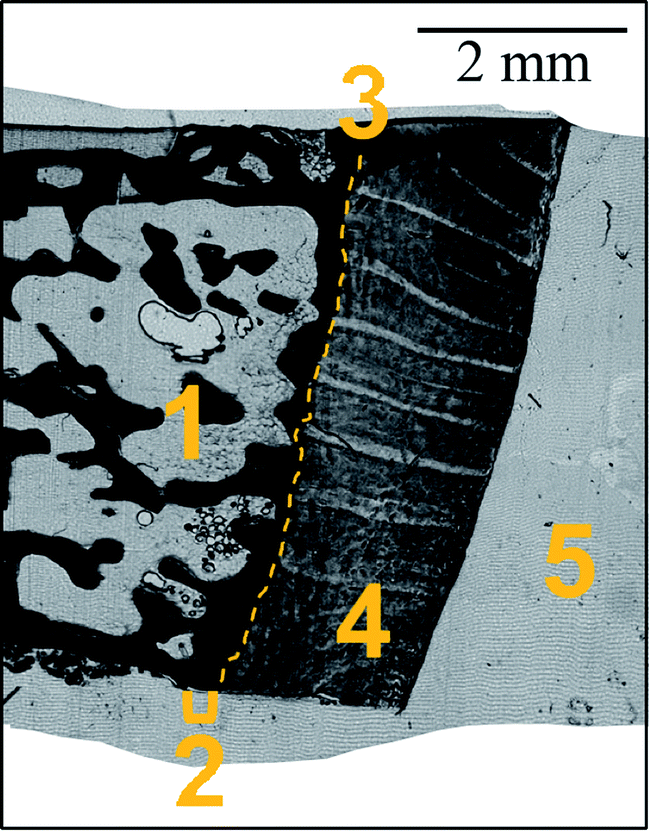 | ||
| Fig. 1 Micrograph (transmitted light microscopy) of an exemplary sample: 1 – trabecular bone (black); 2 – subchondral cortical bone and mineralized cartilage (black); 3 – tidemark (dashed line); 4 – hyaline cartilage; 5 – PMMA outside of the tissue sample. | ||
(2) μXRF measurements, data analysis and quantification
An in-house-built μXRF setup at the Atominstitut, TU Wien, was employed non-confocally (i.e. only one focusing optic, a polycapillary lens – between X-ray tube and sample). More information on the setup can be found in6,21,24 (see also Fig. S1 in ESI†).For the measurements, the samples were sandwiched between acrylic glass frames and attached to a sample holder, which facilitated direct measurement on the sections and eliminated unwanted fluorescent/scattering contributions of backing materials. The samples were positioned vertically in the spectrometer chamber; the standard geometry 45° between the incident radiation beam and the sample, and 90° between the incident beam and the detector was maintained. For these measurements, a Rh-anode low power X-ray tube was used; the tube voltage and current were set to 50 kV and 0.4 mA, respectively. The measurement conditions were: 50 μm step size, 60 s acquisition time per spot (real time), in vacuum (<3 mbar). The step size was chosen due to the estimated beam size of 50 μm (at 8 keV). Deconvolution of the spectra was performed using the QXAS-AXIL software package.25 The original elemental maps were created as text files using the software LP-map26 and processed (negative values zeroed for correct representation) and plotted with ImageJ (version 1.50b).27 The XRF data were dead time corrected. The XRF maps were quantified using the sensitivity values obtained via the measurements of IAEA Animal Bone (H-5) certified reference material, the details can be found in the Master's thesis of V. Pichler.28 The sensitivity values of the elements for which data was not available – sulphur and potassium, were derived by interpolation. The thickness of the cuts was not considered in quantification. The elemental maps, showing the whole scanned area – source images, are included in the ESI.†
For easier comparison and correlation of XRF and LA-ICP-MS data, further analysis by ImageLab (v. 2.99 Epina GmbH, Pressbaum, Austria) was performed (see also below in (3) LA-ICP-MS measurements and data analysis) – and the resultant elemental maps, showing the very same area scanned by both techniques are included in the current manuscript. The original μXRF maps can be found in the ESI.†
Fluorescence sum spectra were plotted with Origin (version OriginPro 2015, OriginLab Corporation, Northampton, MA, USA).
(3) LA-ICP-MS measurements and data analysis
A NWR213 laser ablation system (ESI, Fremont, CA, USA) equipped with a frequency quintupled 213 nm Nd:YAG laser and a fast-washout ablation cell, always held above the actual ablation site, was used for all shown LA-ICP-MS experiments. The device was coupled to an iCAP Q quadrupole ICP-MS instrument (Thermo Fisher Scientific, Bremen, Germany) using PTFE tubing (inner diameter 2 mm). A schematic representation of a general LA-ICP-MS setup is shown on Fig. S1 in ESI.† Helium was used as carrier gas for cell washout, which was mixed with Ar make-up gas upon introduction into the plasma. For data acquisition, Qtegra software provided by the manufacturer of the instrument was used. The tune settings of the MS instrumentation were optimized for maximum 115In signal prior to each experiment using a NIST 612 trace metal in glass standard (National Institute of Standards and Technology, Gaithersberg, MD, USA). Additionally, the oxide ratio was monitored by the 140Ce16O/140Ce ratio, which was below 2.0% for all experiments. To reduce the influence of polyatomic interferences, kinetic energy discrimination (KED) mode utilizing a collision cell containing a mixture of helium with 7% hydrogen was used. A list of potential polyatomic interferences is given in Table S2.†Two-dimensional elemental distribution maps were created using line scan ablation patterns with adjoining lines. In case of the 15 μm slice, an additional pre-ablation step using a similar pattern and reduced laser fluence (4.6 J cm−2) was performed prior to the measurement, removing potential surface contaminations. For image processing, the software ImageLab (v. 2.99 Epina GmbH, Pressbaum, Austria) was used. A pixel size of 25 μm was chosen for the distribution maps, which corresponds to the used laser beam diameter. For plotting the images, interpolated colour surfaces were employed. To evaluate the agreement between obtained maps with the corresponding μXRF images, a correlation analysis was performed using the correlation feature integrated in the software. Detailed information about the used LA-ICP-MS parameters is given in Table 1.
| ESI NWR213 | |
|---|---|
| Average fluence | 11.4 J cm−2 |
| Laser diameter | 25 μm |
| Scan speed | 75 μm s−1 |
| Repetition rate | 20 Hz |
| Carrier gas flow (He) | 0.65 l min−1 |
| Make-up gas flow (Ar) | 0.8 l min−1 |
| Thermo iCAP Q | |
|---|---|
| RF power | 1550 W |
| Plasma gas flow (Ar) | 14 l min−1 |
| Auxiliary gas flow (Ar) | 0.8 l min−1 |
| Collision gas flow (He + 7% H2) | 3 ml min−1 |
| Kinetic energy barrier | 3 V |
| Dwell time per isotope | 10 ms |
| Cones | Ni |
| Measured isotopes | 23Na, 24Mg, 31P, 34S, 39K, 42Ca, 50Cr, 55Mn, 56Fe, 59Co, 64Zn |
Taking into account, that the samples include tissues with significant variations in chemical composition (mineralized tissues and hyaline cartilage), two different standard materials were used for the quantification. While analytes predominately expected in the calcified area (Ca, Mg, Na, P, Zn) were quantified using an IAEA Animal Bone (H-5) certified reference material, a self-made porcine cartilage standard was used for analytes expected in the hyaline cartilage region (K, S). The porcine cartilage standard was characterized via conventional ICP-MS analysis, resulting in K and S contents of 2.46 mg kg−1 ± 0.19 mg kg−1 (![[x with combining macron]](https://www.rsc.org/images/entities/i_char_0078_0304.gif) ± s; n = 3) and 11.1 mg kg−1 ± 1.2 mg kg−1 ( ± s; n = 3), respectively. The sample was digested in a 1/1 volumetric mixture of HNO3 (65 w/w%) and H2O2 (30 w/w%). An iCAP Q ICP-MS instrument (Thermo Fisher Scientific, Bremen, Germany) was used for the analysis. Detailed information about the standard characterization can be found in the ESI.†
± s; n = 3) and 11.1 mg kg−1 ± 1.2 mg kg−1 ( ± s; n = 3), respectively. The sample was digested in a 1/1 volumetric mixture of HNO3 (65 w/w%) and H2O2 (30 w/w%). An iCAP Q ICP-MS instrument (Thermo Fisher Scientific, Bremen, Germany) was used for the analysis. Detailed information about the standard characterization can be found in the ESI.†
The measurement of the standards was performed directly before the imaging experiments using identical instrument and laser settings. Each standard was analysed four times using laser patterns consisting of adjacent line scans. The investigated area was 0.35 mm2 per laser pattern. For further data processing, the mean values of the four-fold analysis were used. To remove potential surface contaminations, a pre-ablation step was performed before the measurements.
Results and discussion
Local elemental distributions were obtained from the measurement areas, which were chosen such as to include bone, articular cartilage tissue and the metabolically active area of tidemark – the interface between calcified and non-calcified cartilage; the elemental maps of 15 μm and 41 μm cuts are shown on Fig. 2 and 3, respectively. These figures show the very same area within each slice imaged by μXRF and LA-ICP-MS (further details are provided in the text below).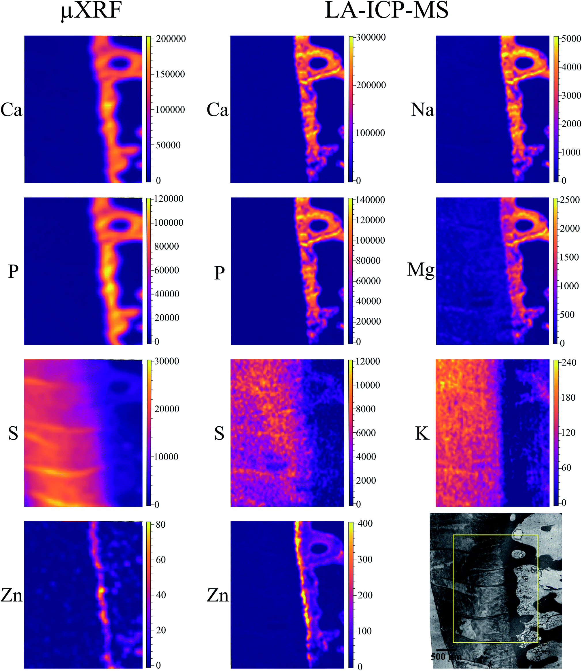 | ||
| Fig. 2 15 μm slice: elemental maps obtained by μXRF and LA-ICP-MS. The micrograph (transmitted light microscopy) in the low right corner shows the scanned region (yellow rectangle). The units for both μXRF and LA-ICP-MS maps are μg g−1. Please note, that S μXRF map is subject to fitting artifact within mineralized tissue (no S actually detected), detailed explanation is provided in the text. | ||
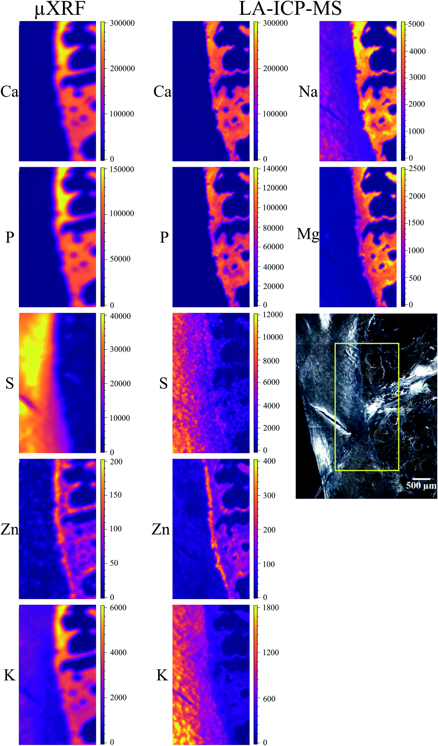 | ||
| Fig. 3 41 μm slice: elemental maps obtained by μXRF and LA-ICP-MS. The micrograph shows the scanned region (yellow rectangle). The units for both μXRF and LA-ICP-MS maps are μg g−1. Please note, that K μXRF map is subject to fitting artifact within mineralized tissue (no K actually detected), detailed explanation is provided in the text. | ||
μXRF
The sum spectra (generated by adding spectra from each measured point) obtained from μXRF scans of two cuts are shown in Fig. 4. High content of Ca and P corresponds to the bone and calcified cartilage area, while high S peak can be attributed to the hyaline cartilage. Zn, Pb and Sr are expected to be found in the sample (Zn in both cartilage and bone, accumulation of Zn and Pb in tidemark, Sr – in bone), although Pb and Sr peaks are hardly discernible, therefore, these metals were excluded from further analysis. Fe, although normally present in tissues (e.g. from blood), can also be introduced in the sample by the cutting equipment, therefore, Fe, Co, as well as Ti and Cr (only found in the 41 μm cut) were considered contaminations. Interestingly, in the sum spectrum of 41 μm cut, peak of K can be recognised on the left shoulder of Ca-Kα peak.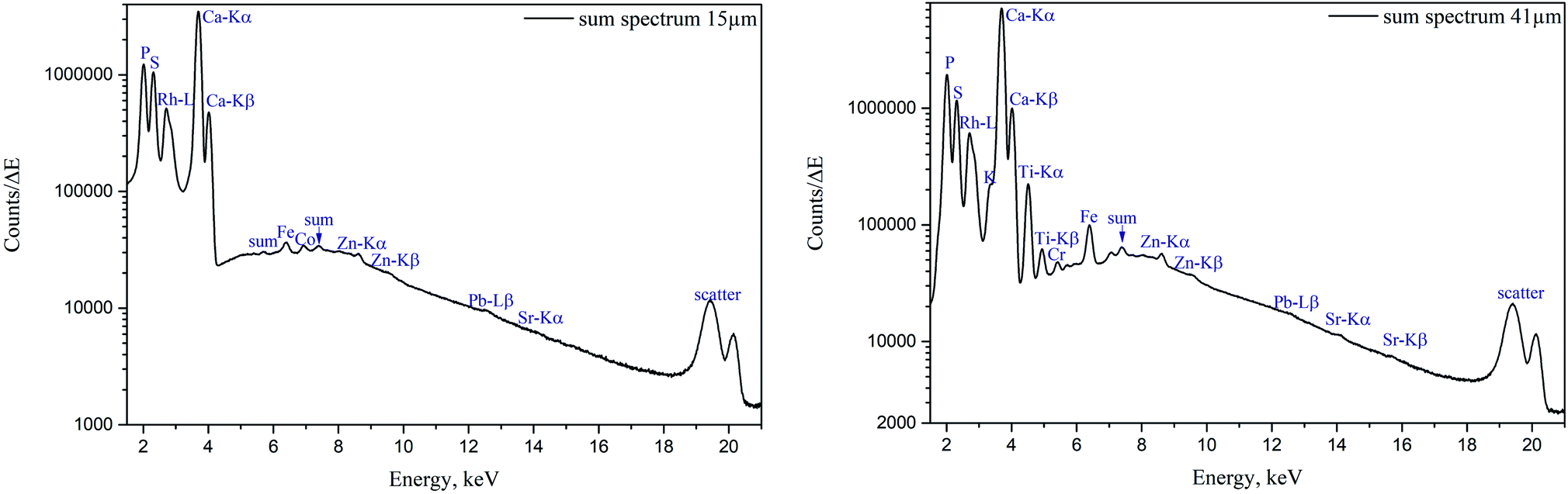 | ||
| Fig. 4 μXRF sum spectra of human femoral head sample; left – 15 μm cut, right – 41 μm cut. | ||
Fig. 2 and 3 show segments of the scans performed on the 15 μm cut and 41 μm cut, respectively, to match the areas imaged by both methods. The whole μXRF scans are included in the ESI (Fig. S2 and S3†). A detailed description of the μXRF results provided below is based on the original μXRF maps. Please note that the values discussed further in this section originate from the Tables S3 and S4 in the ESI.†
Sulphur is present exclusively in the hyaline cartilage with an average concentration of ca. 17 mg g−1. It should be noted that the presence of S (values ≤4 mg g−1) within calcified tissues occurs due to a spectral artifact: the high Ca signal causes an escape peak of Ca-Kβ line at 2.27 keV. This artificial peak has similar energy to S (2.3 keV), therefore fitting software misrelates the signal. The line structures, which can be seen within the hyaline cartilage in microscopy picture and also in the S map correspond to the folds on the sample surface. The concentrations of S and Ca in the folds are nearly two times higher than in the surrounding tissue.
Zn is present in bone and, in higher content in the tidemark zone. The estimated mean Zn concentration is 15 μg g−1 in bone and 50 μg g−1 in tidemark.
Average S content in hyaline cartilage is around 27 mg g−1. The maps are subject to the same fitting problem for S in the presence of high Ca content as described above for the 15 μm slice. However, unlike the 15 μm slice, S distribution was confirmed in the voids of trabecular bone, its origin remains unknown.
Zn is detected in bone, as well as in tidemark, where the concentration reaches 150–200 μg g−1. When comparing Zn XRF maps of the two slices, it can be seen that overall a more distinct Zn distribution was obtained for the thicker sample. However, the differentiation between bone and tidemark in the 41 μm cut is not as clear as in 15 μm slice. This can be understood considering that the theoretical information depth for Zn is about 98 μm. Therefore, in both cuts the signal from the entire sample thickness is obtained – albeit stronger in 41 μm slice. In the thicker sample the information depth contributes also to the smearing effect for such a thin structure as tidemark, making tidemark in 41 μm sample less pronounced than in the 15 μm cut.
K is present in the hyaline cartilage of the 41 μm slice, and there is a clear separated peak of K in corresponding spectra. The average K concentration in hyaline cartilage is 1.3 mg g−1. The K map seems to exhibit a higher K signal in the calcified zone, however in reality we are unable to confirm this element in mineralized tissue. This effect is caused again by intense Ca signal, in this case false-positive fitting of K occurs in tail of high Ca-Kα peak.
For the interpretation of the results, it is important to note, that in the μXRF maps the depth resolution is element-dependent, and (in case of thin sections discussed in present paper) often is the representation of the signal from the entire sample thickness. In cortical bone, for example, it can be estimated as 9 μm for P; 39 μm for Ca and 98 μm for Zn, using the mass attenuation coefficients for cortical bone (μ/ρ)29 and the theoretical density for cortical bone of 1.92 g cm−3.30 This is the reason why maximum Ca value in 41 μm slice is about 50% higher than in the 15 μm slice. Further, the information depth will be different for bone and hyaline cartilage, as it depends strongly on the actual material composition. An approximation for the information depth values in cartilage can be obtained using the mass attenuation coefficients for soft tissue29 and the theoretical density for cartilage of 1.1 g cm−3 (ref. 30) as 16 μm for P, 24 μm for S, 50 μm for K, 111 μm for Ca and 872 μm for Zn. Quantification of cartilaginous zone by using IAEA Animal Bone (H-5) certified reference material (for μXRF, see Materials and methods) is, therefore, not optimal. Unfortunately, cartilage certified reference material is not commercially available, and, thus, a well-characterized homogenous standard material (optionally doped with specific elements) will be beneficial in future measurements.
LA-ICP-MS
Major elements (Ca, Mg, Na, K, P, S) as well as minor/trace elements (Co, Cr, Fe, Mn, Zn) expected to be found in a sample were included in the LA-ICP-MS analysis. Although C is measurable with ICP-MS, it was excluded from the analysis since the C-rich embedding medium would falsify the analysis. For each analyte, one isotope was chosen using absence of potential (isobaric and polyatomic) interferences as well as natural abundance as selection criteria. We assume that the information depth of the LA-ICP-MS measurements is about 5 μm, it is similar for both slices independently of their thickness, and only varies among different histological areas, i.e. mineralized tissues and hyaline cartilage.50Cr and 55Mn did not provide sufficient signal-to-noise ratios for the generation of elemental maps and were therefore excluded from further analysis. 56Fe and 59Co show significant signal intensities in some sample areas, however, since they most likely originate from contaminations due to sample preparation they were excluded from further analysis as well. The elemental maps of the remaining analytes were quantified via external calibration using the measured IAEA Animal Bone (H-5) certified reference material as well as the self-made porcine cartilage standard. To keep matrix effects as small as possible, those analytes predominately in the calcified area (42Ca, 24Mg, 23Na, 31P, 64Zn) were quantified using the bone standard, while the cartilage standard was used for those analytes predominately in the hyaline cartilage area (34S, 39K). This means that the analysis is not perfectly matrix-matched for the tissue in which the analyte shows lower concentration (e.g. Ca in hyaline cartilage tissue). However, since the presence of most elements is rather limited to one kind of tissue (e.g. Ca in mineralized tissue), the resulting error is hardly visible in the elemental maps and therefore negligible. Image quantification was performed without internal standard correction since no element suitable as internal standard (i.e. constant concentration in whole sample) was available. Finding a way for utilizing internal standardization to compensate differences in material ablation and instrumental drifts could potentially further improve the accuracy of the analysis.
The LA-ICP-MS elemental maps (cf.Fig. 2, 3, Tables 2 and 3) show high Ca and P concentrations (ca. 170 mg g−1 and 75 mg g−1, respectively) as well as significant Na, Mg, and Zn content (ca. 3 mg g−1, 1.3 mg g−1, and 140 μg g−1, respectively) in the calcified zone of the sample. In case of Zn, there is a significant enrichment in the tidemark zone (up to ca. 400 μg g−1) visible. In case of Na, the map of the 41 μm slice shows also a relatively high concentration in the hyaline cartilage area, which cannot be observed for the 15 μm sample. Since a pre-ablation step was performed for the later one (for cleaning purposes; see Experimental), the Na measured in the hyaline cartilage tissue of the 41 μm slice probably originates from surface contaminations.
± s)
| 15 μm | Mineralized tissue (Ca (XRF) >100 mg g−1) | |
|---|---|---|
| LA-ICP-MS | μXRF | |
|
± s |
± s |
|
| Ca | 171 ± 77 mg g−1 | 137 ± 19 mg g−1 |
| K | <LOD | — |
| Mg | 1.3 ± 0.6 mg g−1 | — |
| Na | 3 ± 1.4 mg g−1 | — |
| P | 77 ± 36 mg g−1 | 90 ± 13 mg g−1 |
| S | <LOQ | — |
| Zn | 139 ± 115 μg g−1 | 12 ± 17 μg g−1 |
| 15 μm | Cartilage (hyaline) (S (XRF) >10 mg g−1) | |
|---|---|---|
| LA-ICP-MS | μXRF | |
|
± s |
± s |
|
| Ca | 3.5 ± 1.6 mg g−1 | 2.6 ± 5.6 mg g−1 |
| K | <LOQ | — |
| Mg | 194 ± 76 μg g−1 | — |
| Na | 100 ± 42 μg g−1 | — |
| P | <LOD | 1.4 ± 3.5 mg g−1 |
| S | 6 ± 1.9 mg g−1 | 17 ± 3.5 mg g−1 |
| Zn | 7 ± 4 μg g−1 | 1 ± 4 μg g−1 |
± s)
| 41 μm | Mineralized tissue (Ca (XRF) >100 mg g−1) | |
|---|---|---|
| LA-ICP-MS | μXRF | |
|
± s |
± s |
|
| Ca | 162 ± 68 mg g−1 | 193 ± 45 mg g−1 |
| K | <LOQ | — |
| Mg | 1.5 ± 0.6 mg g−1 | — |
| Na | 3.5 ± 1.3 mg g−1 | — |
| P | 72 ± 31 mg g−1 | 102 ± 25 mg g−1 |
| S | <LOQ | — |
| Zn | 145 ± 68 μg g−1 | 94 ± 32 μg g−1 |
| 41 μm | Cartilage (hyaline) (S (XRF) >10 mg g−1) | |
|---|---|---|
| LA-ICP-MS | μXRF | |
|
± s |
± s |
|
| Ca | 7 ± 30 mg g−1 | 8 ± 23 mg g−1 |
| K | 1 ± 0.4 mg g−1 | 1.3 ± 0.5 mg g−1 |
| Mg | 174 ± 193 μg g−1 | — |
| Na | 1.5 ± 0.7 mg g−1 | — |
| P | 2.3 ± 14 mg g−1 | 3.9 ± 12.5 mg g−1 |
| S | 5.9 ± 2.2 mg g−1 | 27 ± 6.7 mg g−1 |
| Zn | 42 ± 34 μg g−1 | 17 ± 22 μg g−1 |
For the areas consisting of hyaline cartilage tissue, a relatively high S content (up to 12 mg g−1) can be observed. Despite S being a main constituent, the image quality is rather poor, which is caused by the relatively high ionization energy of S, the fact that the main S isotope (32S) cannot be measured due to polyatomic interferences (O2+ species), and a relatively high S-background caused by the applied ablation chamber and tubing system. Beside S also K can predominately be observed in the hyaline cartilage tissue (0.2–1.5 mg g−1). Even though the measurement of K suffers from a high background due to interferences originating from the plasma gas (38Ar1H+), the quality of the obtained images is sufficient.
Method correlation
Since every analytical technique has certain requirements to the samples, the first challenge was to choose a sample preparation approach compatible with both imaging methods. In our experiments, PMMA embedding resulted in self-supporting thin sections, which allowed direct analysis with μXRF; and acrylic glass frames ensured that the sample is flattened during the measurement. After the non-destructive μXRF measurements, an intact sample was transferred to LA-ICP-MS instrument. For LA-ICP-MS measurements sample was glued onto a plastic slide using sticky tape on the edges of the sample – similarly, to straighten and fix the sample horizontally; no other sample handling manipulations were required. While the method of PMMA embedding is routinely used in bone samples preparation, it is worth mentioning, that the preservation of hyaline cartilage in the same way might not be optimal and some elements (diffusible ions, like Na+ and K+) might have been washed out or relocated.31 Further investigations and more refined sample preparation techniques (e.g. cryofixation/freeze-drying) are needed to obtain the information on chemical distribution within the non-mineralized cartilage in near-natural state.Due to the non-destructive character of μXRF, these measurements were performed first. An advantage of this experimental order is that μXRF results provide guidance for the elements of interest in subsequent LA-ICP-MS analysis. In our experiments we first focused on the expected major elements, which could be measured by both μXRF and LA-ICP-MS. In addition LA-ICP-MS provided the images for light metals – Na and Mg, which could not be imaged by laboratory μXRF due to limitations of the measuring system (e.g. detector window transmission).
We obtained quantitative maps with both methods, the employed quantification approach resulted in the concentrations in the same order of magnitude for the investigated elements imaged by both μXRF and LA-ICP-MS. To directly compare the elemental concentrations obtained by μXRF and LA-ICP-MS within the very same areas imaged by both techniques, we subdivided the maps shown in Fig. 2 and 3 in two subsections – mineralized tissue (selection criteria: Ca value in μXRF map > 100 mg g−1) and hyaline cartilage (selection criteria: S value in μXRF map >10 mg g−1). The averaged values and standard deviation for the elements within these subsections are presented in Table 2 (15 μm slice) and Table 3 (41 μm slice).
Generally for μXRF, it should be noted that the excited/detected sample mass in 15 μm is lower than in 41 μm, which leads to different concentration values. As LA-ICP-MS is not affected by sample thickness, similar values are observed for 15 μm and 41 μm slices, except for K – which is notably higher in the 41 μm slice. Specifically for K, it should be emphasized, that this element could be detected by μXRF only in the 41 μm slice in cartilage – here we assume the influence of larger sampling volume in thicker sample. The μXRF mean cartilage value for potassium corresponds to the potassium content reported by LA-ICP-MS.
Since S maps are more detailed in μXRF measurements, we conclude that LA-ICP-MS is less sensitive to S, most likely due to the previously mentioned high S-background (cf. the estimated detection limits included in ESI, Table S5†). In case of Zn, LA-ICP-MS provided more detailed distribution maps for both samples – more features can be seen in slice 15 μm in comparison to μXRF; in slice 41 μm the histological structures are clearer, due to higher depth resolution of LA-ICP-MS.
To further evaluate the agreement between the images obtained by μXRF and LA-ICP-MS, we calculated the correlation between the corresponding elemental maps on Fig. 2 and 3. We used the Pearson correlation coefficient for the evaluation. It assumes values in the range from −1 to +1, where 1 indicates strongest possible agreement, 0 strongest possible disagreement, and −1 perfect negative correlation. Table 4 displays the result – Pearson correlation coefficients calculated for each analyte obtained by μXRF and LA-ICP-MS. Overall, lower coefficients were obtained for 15 μm compared to 41 μm sample. In case of Ca and P, the method shows excellent agreement with high correlation coefficients for both samples. Also for S and Zn strong correlations can be observed, especially in 41 μm slice. The only analyte showing poor correlation is K. The reason for that is imperfect μXRF spectra fitting, leading to false-positive K distribution in calcified zone (see above), ultimately resulting in mismatched elemental map and, consequently, poor correlation. With the exception of K, the correlation analysis confirms that the μXRF and LA-ICP-MS images are in good agreement.
Although many studies have been published on elemental distribution analyses of human bone with XRF-based methods, we were unable to find reports on quantitative mapping (absolute quantification). Papers on quantitative imaging with use of LA-ICP-MS exist, albeit limited to archaeological objects.32,33
Quantitative elemental analysis of bone will be of interest for the diagnostic reasons, for example, investigation of Sr incorporation from strontium ranelate with implications for the quality of the mineral crystal;34 quantification of trace element accumulations (Zn) in the tumorous tissue3 or estimation of metal transfer from orthopaedic implants.35 We have recently reported accumulations of elements-xenobiotics, e.g. lead in tidemark8 and gadolinium in bone,36 and quantification could help in assessing the risk of potential re-release of those elements in bloodstream.
As for rather neglected area of cartilage analysis, most of the elemental imaging experiments with LA-ICP-MS or μXRF found in literature were performed qualitatively on the animal tissues. This limits the direct comparison to our results; nonetheless, these published findings point out other chemical elements, which should be considered in future measurements. Sussulini et al. imaged bovine cartilage by means of LA-ICP-MS, and in addition to Na, Mg, P, S, K, Ca, and Zn, also C, Cl, Ti and Cu were detected in articular cartilage tissues.37 Whereas C and Cl are expected as intrinsic components of biological tissues, Ti is normally not present in cartilage and in our sample (41 μm) was considered as contamination. Cu, however, is an essential element and was also detected and imaged in dried droplet of synovial fluid of osteoarthritic patient by Austin et al.38 The authors also report distribution of Ca, P, Mg, Sr and Zn in a knee cartilage section of OA patient. Notably, Austin et al. used thin samples for the experiments – dried 14 μm sections, without any other treatment – which seemingly resulted in folding and twisting of the tissue. In our study, we observed only few cartilage folds in the thinner, 15 μm sample, otherwise PMMA embedding facilitated preserving the overall shape of the tissue.
Reinert et al. obtained distributions of P, S, Cl, K and Ca in articular cartilage of juvenile pig's knee joint using particle induced X-ray emission (PIXE).39 They reported variations in S distribution within different histological zones, consistent with proteoglycan content, positively correlated with K, and displaying maximum concentration in hypertrophic cartilage (zone of hyaline cartilage contiguous to tidemark). Further, Reinert et al. detected calcium–phosphorus accumulation within the superficial cartilage. None of these was observed in our experiments. These dissimilarities could be attributed to the origin of the sample – animal vs. human; or the sample preparation – freeze-drying by Reinert et al. and PMMA embedding in our case.
In future, adding histological analysis for detailed assignment of the cartilaginous zones and coupling elemental imaging with molecular (e.g. MALDI) could be beneficial. Human bone sample preparation allowing preservation of biomolecules (lipids) followed by consecutive time-of-flight secondary ion mass spectrometry (TOF-SIMS) and atmospheric pressure scanning microprobe matrix assisted laser desorption/ionization (AP-SMALDI) molecular imaging have been recently presented by Schaepe et al.40 Knowledge on distributions and content of certain elements in human tissues will further histopathological studies. For instance, the elemental imaging of bone and cartilage will be of use for investigation of Ca deposits and crystals in cartilage, as well as osteoarthritic lesions.41,42
The presented spatial distribution of elements accompanied by absolute quantitative data is an exceptional combination in human bone and cartilage analysis, and we hope that our research will serve as a base for future studies in this area.
Conclusions
The current paper presents the analysis by two elemental imaging techniques – μXRF and LA-ICP-MS – of a complex human bone-cartilage sample (femoral head). The measurements were performed in consecutive manner on the very same sample surfaces of two slices. Quantitative distribution mapping for both μXRF and LA-IPC-MS was performed with the use of matrix-matched standards, and the concentrations obtained by both methods are either similar or at least in the same order of magnitude. We report concentrations for various elements within different histological zones – e.g. mineralized tissues, tidemark, hyaline cartilage. Further, we compared LA-ICP-MS and μXRF by means of correlation analysis applied to elemental maps, and observed strong (Ca, P in both samples, and S, Zn in 41 μm slice) or good (S and Zn in 15 μm slice) correlation of the methods. We believe that this is the first holistic description – imaging of elemental distribution supported by quantitative data – of bone and cartilage by either of the methods. Combined sequential application of μXRF and LA-ICP-MS within one sample offers additional benefits, and should be further applied in the biomedical research.Conflicts of interest
There are no conflicts of interest to declareAcknowledgements
Authors thank Prof. Heinrich W Thaler for providing the samples. Authors would like to thank Dr Stéphane Blouin for support and EDX analysis of sample preparation tools, and technicians of LBIO for careful sample preparation. Authors gratefully acknowledge the help provided by Angelica de Leon (for cartilage preparation and characterization by XRF), Lukas Fenninger (for XRF measurements of cartilage pellets), Alexander Kleeweiss (for XRF measurements of cartilage pellets, fused beads), and Maximilian Bonta (for running trial test on a sample with LA-ICP-MS). AT and MR were supported by the FWF (The Austrian Science Fund) Project P 27715. AT also received support within MEIBio (Molecular and Elemental Imaging in Biosciences) PhD program of TU Wien. The authors acknowledge TU Wien Bibliothek for financial support through its Open Access Funding Programme.References
- D. S. Gholap, A. Izmer, B. De Samber, J. T. van Elteren, V. S. Šelih, R. Evens, K. De Schamphelaere, C. Janssen, L. Balcaen, I. Lindemann, L. Vincze and F. Vanhaecke, Comparison of laser ablation-inductively coupled plasma-mass spectrometry and micro-X-ray fluorescence spectrometry for elemental imaging in Daphnia magna, Anal. Chim. Acta, 2010, 664, 19–26 Search PubMed.
- A. Al-Ebraheem, K. Geraki, R. Leek, A. L. Harris and M. J. Farquharson, The use of bio-metal concentrations correlated with clinical prognostic factors to assess human breast tissues, X-Ray Spectrom., 2013, 42, 330–336 Search PubMed.
- M. Rauwolf, B. Pemmer, A. Roschger, A. Turyanskaya, S. Smolek, A. Maderitsch, P. Hischenhuber, M. Foelser, R. Simon, S. Lang, S. E. Puchner, R. Windhager, K. Klaushofer, P. Wobrauschek, J. G. Hofstaetter, P. Roschger and C. Streli, Increased zinc accumulation in mineralized osteosarcoma tissue measured by confocal synchrotron radiation micro X-ray fluorescence analysis, X-Ray Spectrom., 2017, 46, 56–62 Search PubMed.
- A. Gaál, G. Orgován, V. G. Mihucz, I. Pape, D. Ingerle, C. Streli and N. Szoboszlai, Metal transport capabilities of anticancer copper chelators, J. Trace Elem. Med. Biol., 2018, 47, 79–88 Search PubMed.
- B. Pemmer, A. Roschger, A. Wastl, J. G. Hofstaetter, P. Wobrauschek, R. Simon, H. W. Thaler, P. Roschger, K. Klaushofer and C. Streli, Spatial distribution of the trace elements zinc, strontium and lead in human bone tissue, Bone, 2013, 57, 184–193 Search PubMed.
- A. Turyanskaya, M. Rauwolf, T. Grünewald, M. Meischel, S. Stanzl-Tschegg, J. Löffler, P. Wobrauschek, A. Weinberg, H. Lichtenegger and C. Streli, μXRF Elemental Mapping of Bioresorbable Magnesium-Based Implants in Bone, Materials, 2016, 9, 811 Search PubMed.
- N. Zoeger, C. Streli, P. Wobrauschek, C. Jokubonis, G. Pepponi, P. Roschger, J. Hofstaetter, A. Berzlanovich, D. Wegrzynek, E. Chinea-Cano, A. Markowicz, R. Simon and G. Falkenberg, Determination of the elemental distribution in human joint bones by SR micro XRF, X-Ray Spectrom., 2008, 37, 3–11 Search PubMed.
- A. Roschger, J. G. Hofstaetter, B. Pemmer, N. Zoeger, P. Wobrauschek, G. Falkenberg, R. Simon, A. Berzlanovich, H. W. Thaler, P. Roschger, K. Klaushofer and C. Streli, Differential accumulation of lead and zinc in double-tidemarks of articular cartilage, Osteoarthritis and Cartilage, 2013, 21, 1707–1715 Search PubMed.
- N. Zoeger, P. Roschger, J. G. Hofstaetter, C. Jokubonis, G. Pepponi, G. Falkenberg, P. Fratzl, A. Berzlanovich, W. Osterode, C. Streli and P. Wobrauschek, Lead accumulation in tidemark of articular cartilage, Osteoarthritis and Cartilage, 2006, 14, 906–913 Search PubMed.
- K. Geraki, M. J. Farquharson, D. A. Bradley, O. Gundogdu and G. Falkenberg, The localisation of biologically important metals in soft and calcified tissues using a synchrotron x-ray fluorescence technique, X-Ray Spectrom., 2008, 37, 12–20 Search PubMed.
- A. Boyde, F. A. Mccorkell, G. K. Taylor, R. J. Bomphrey and M. Doube, Iodine vapor staining for atomic number contrast in backscattered electron and X-ray imaging, Microsc. Res. Tech., 2014, 77, 1044–1051 Search PubMed.
- B. Pouran, V. Arbabi, A. G. Bajpayee, J. van Tiel, J. Töyräs, J. S. Jurvelin, J. Malda, A. A. Zadpoor and H. Weinans, Multi-scale imaging techniques to investigate solute transport across articular cartilage, J. Biomech., 2018, 78, 10–20 Search PubMed.
- A. Limbeck, P. Galler, M. Bonta, G. Bauer, W. Nischkauer and F. Vanhaecke, Recent advances in quantitative LA-ICP-MS analysis: Challenges and solutions in the life sciences and environmental chemistry ABC Highlights: Authored by Rising Stars and Top Experts, Anal. Bioanal. Chem., 2015, 407, 6593–6617 Search PubMed.
- R. Zhang, L. Li, Y. Sultanbawa and Z. P. Xu, X-ray fluorescence imaging of metals and metalloids in biological systems, Am. J. Nucl. Med. Mol. Imagingc, 2018, 8, 169–188 Search PubMed.
- D. S. Urgast, J. H. Beattie and J. Feldmann, Imaging of trace elements in tissues: With a focus on laser ablation inductively coupled plasma mass spectrometry, Curr. Opin. Clin. Nutr. Metab. Care, 2014, 17, 431–439 Search PubMed.
- D. Pozebon, G. L. Scheffler and V. L. Dressler, Recent applications of laser ablation inductively coupled plasma mass spectrometry (LA-ICP-MS) for biological sample analysis: A follow-up review, J. Anal. At. Spectrom., 2017, 32, 890–919 Search PubMed.
- K. M. Davies, D. J. Hare, S. Bohic, S. A. James, J. L. Billings, D. I. Finkelstein, P. A. Doble and K. L. Double, Comparative Study of Metal Quantification in Neurological Tissue Using Laser Ablation-Inductively Coupled Plasma-Mass Spectrometry Imaging and X-ray Fluorescence Microscopy, Anal. Chem., 2015, 87, 6639–6645 Search PubMed.
- J.-C. Müller, M. Horstmann, L. Traeger, A. U. Steinbicker, M. Sperling and U. Karst, μXRF and LA-ICP-TQMS for quantitative bioimaging of iron in organ samples of a hemochromatosis model, J. Trace Elem. Med. Biol., 2019, 52, 166–175 Search PubMed.
- A. Balbekova, M. Bonta, S. Török, J. Ofner, B. Döme, A. Limbeck and B. Lendl, FTIR-spectroscopic and LA-ICP-MS imaging for combined hyperspectral image analysis of tumor models, Anal. Methods, 2017, 9, 5464–5471 Search PubMed.
- M. Holzlechner, M. Bonta, H. Lohninger, A. Limbeck and M. Marchetti-Deschmann, Multisensor Imaging - From Sample Preparation to Integrated Multimodal Interpretation of LA-ICPMS and MALDI MS Imaging Data, Anal. Chem., 2018, 90, 8831–8837 Search PubMed.
- A. Svirkova, A. Turyanskaya, L. Perneczky, C. Streli and M. Marchetti-Deschmann, Multimodal imaging of undecalcified tissue sections by MALDI MS and μXRF, Analyst, 2018, 143, 2587–2595 Search PubMed.
- S. Blouin, H. W. Thaler, C. Korninger, R. Schmid, J. G. Hofstaetter, R. Zoehrer, R. Phipps, K. Klaushofer, P. Roschger and E. P. Paschalis, Bone matrix quality and plasma homocysteine levels, Bone, 2009, 44, 959–964 Search PubMed.
- P. Roschger, P. Fratzl, J. Eschberger and K. Klaushofer, Validation of quantitative backscattered electron imaging for the measurement of mineral density distribution in human bone biopsies, Bone, 1998, 23, 319–326 Search PubMed.
- S. Smolek, B. Pemmer, M. Fölser, C. Streli and P. Wobrauschek, Rev. Sci. Instrum., 2012, 83, 083703 Search PubMed.
- International Atomic Energy Agency (IAEA), 2009, https://www.iaea.org/publications/7884/quantitative-x-ray-analysis-system.
- L. Perneczky, Implementation of a confocal synchrotron radiation induced micro X-ray fluorescence system for bone analysis at the X-ray fluorescence beamline of ELETTRA synchrotron, Master's thesis, TU Wien, 2018. http://hdl.handle.net/20.500.12708/3465.
- C. A. Schneider, W. S. Rasband and K. W. Eliceiri, NIH Image to ImageJ: 25 years of image analysis, Nat. Methods, 2012, 9, 671–675 Search PubMed.
- V. Pichler, Ansätze zur Quantifizierung in der Mikro-XRF-Analyse unter Verwendung eines speziellen Spektrometers für leichte Elemente, Master's thesis, TU Wien, 2019, http://hdl.handle.net/20.500.12708/2013.
- J. H. Hubbell and S. M. Seltzer, Tables of X-Ray Mass Attenuation Coefficients and Mass Energy-Absorption Coefficients from 1 keV to 20 MeV for Elements Z = 1 to 92 and 48 Additional Substances of Dosimetric Interest. X-Ray Mass Attenuation Coefficients, NIST Standard Reference Database, https://physics.nist.gov/PhysRefData/XrayMassCoef/tab4.html Search PubMed.
- D. R. White, J. Booz, R. V. Griffith, J. J. Spokas and I. J. Wilson, Report 44, Tissue substitutes in radiation dosimetry and measurement, 1989, vol. os23 Search PubMed.
- M. J. Hackett, J. A. McQuillan, F. El-Assaad, J. B. Aitken, A. Levina, D. D. Cohen, R. Siegele, E. A. Carter, G. E. Grau, N. H. Hunt and P. A. Lay, Chemical alterations to murine brain tissue induced by formalin fixation: implications for biospectroscopic imaging and mapping studies of disease pathogenesis, Analyst, 2011, 136, 2941 Search PubMed.
- A.-F. Maurer, P. Barrulas, A. Person, J. Mirão, C. Barrocas Dias, O. Boudouma and L. Segalen, Testing LA-ICP-MS analysis of archaeological bones with different diagenetic histories for paleodiet prospect, Palaeogeogr., Palaeoclimatol., Palaeoecol., 2019, 534, 109287 Search PubMed.
- K. L. Rasmussen, G. Milner, L. Skytte, N. Lynnerup, J. L. Thomsen and J. L. Boldsen, Mapping diagenesis in archaeological human bones, Heritage Sci., 2019, 7, 41 Search PubMed.
- C. Li, O. Paris, S. Siegel, P. Roschger, E. P. Paschalis, K. Klaushofer and P. Fratzl, Strontium is incorporated into mineral crystals only in newly formed bone during strontium ranelate treatment, J. Bone Miner. Res., 2010, 25, 968–975 Search PubMed.
- F. Bilo, L. Borgese, J. Prost, M. Rauwolf, A. Turyanskaya, P. Wobrauschek, P. Kregsamer, C. Streli, U. Pazzaglia and L. E. Depero, Atomic layer deposition to prevent metal transfer from implants: An X-ray fluorescence study, Appl. Surf. Sci., 2015, 359, 215–220 Search PubMed.
- A. Turyanskaya, M. Rauwolf, V. Pichler, R. Simon, M. Burghammer, O. J. L. Fox, K. Sawhney, J. G. Hofstaetter, A. Roschger, P. Roschger, P. Wobrauschek and C. Streli, Detection and imaging of gadolinium accumulation in human bone tissue by micro- and submicro-XRF, Sci. Rep., 2020, 10, 6301 Search PubMed.
- A. Sussulini, E. Wiener, T. Marnitz, B. Wu, B. Müller, B. Hamm and J. Sabine Becker, Quantitative imaging of the tissue contrast agent [Gd(DTPA)]2- in articular cartilage by laser ablation inductively coupled plasma mass spectrometry, Contrast Media Mol. Imaging, 2013, 8, 204–209 Search PubMed.
- C. Austin, D. Hare, A. L. Rozelle, W. H. Robinson, R. Grimm and P. Doble, Elemental bio-imaging of calcium phosphate crystal deposits in knee samples from arthritic patients, Metallomics, 2009, 1, 142 Search PubMed.
- T. Reinert, U. Reibetanz, M. Schwertner, J. Vogt, T. Butz and A. Sakellariou, The architecture of cartilage: Elemental maps and scanning transmission ion microscopy/tomography, Nucl. Instrum. Methods Phys. Res., Sect. B, 2002, 188, 1–8 Search PubMed.
- K. Schaepe, D. R. Bhandari, J. Werner, A. Henss, A. Pirkl, M. Kleine-Boymann, M. Rohnke, S. Wenisch, E. Neumann, J. Janek and B. Spengler, Imaging of Lipids in Native Human Bone Sections Using TOF-Secondary Ion Mass Spectrometry, Atmospheric Pressure Scanning Microprobe Matrix-Assisted Laser Desorption/Ionization Orbitrap Mass Spectrometry, and Orbitrap-Secondary Ion Mass Spectrometry, Anal. Chem., 2018, 90, 8856–8864 Search PubMed.
- W. Kaabar, O. Gundogdu, a. Laklouk, O. Bunk, F. Pfeiffer, M. J. Farquharson and D. a Bradley, Micro-PIXE and SAXS studies at the bone-cartilage interface, Appl. Radiat. Isot., 2010, 68, 730–734 Search PubMed.
- W. Kaabar, a. Laklouk, O. Bunk, M. Baily, M. J. Farquharson and D. Bradley, Compositional and structural studies of the bone–cartilage interface using PIXE and SAXS techniques, Nucl. Instrum. Methods Phys. Res., Sect. A, 2010, 619, 78–82 Search PubMed.
Footnote |
| † Electronic supplementary information (ESI) available. See DOI: 10.1039/d1ja00007a |
| This journal is © The Royal Society of Chemistry 2021 |