
Quantitative prediction of rare earth concentrations in salt matrices using laser-induced breakdown spectroscopy for application to molten salt reactors and pyroprocessing†
Gregory
Hull
 *ab,
Hugues
Lambert
ac,
Kiran
Haroon
a,
Paul
Coffey
ab,
Timothy
Kerry
ad,
Edward D.
McNaghten
e,
Clint A.
Sharrad
a and
Philip
Martin
*ab
*ab,
Hugues
Lambert
ac,
Kiran
Haroon
a,
Paul
Coffey
ab,
Timothy
Kerry
ad,
Edward D.
McNaghten
e,
Clint A.
Sharrad
a and
Philip
Martin
*ab
aDepartment of Chemical Engineering and Analytical Science, University of Manchester, Oxford Road, Manchester, M13 9PL, UK. E-mail: Gregory.Hull@postgrad.manchester.ac.uk; Philip.Martin@manchester.ac.uk
bPhoton Science Institute, University of Manchester, Oxford Road, Manchester, M13 9PL, UK
cLhoist – Business Innovation Center, 31 rue de l'industrie, 1400 Nivelles, Belgium
dDepartment of Materials Science and Engineering, Delft University of Technology, Mekelweg 2, CD Delft, 2628, The Netherlands
eAWE, Aldermaston, Reading, Berkshire RG7 4PR, UK
First published on 10th November 2020
Abstract
Pyroprocessing of spent nuclear fuels is an electrochemical separation method where spent metallic fuel is dissolved in a molten salt bath to allow uranium (U) and plutonium (Pu) to be isolated from fission products (FPs) and other impurities. This allows the useful materials to be reused in mixed oxide fuel (MOx) or further refined to new reactor fuel. Monitoring the changing concentrations of U, Pu, FPs and other species inside a molten salt vessel presents a unique challenge which laser-induced breakdown spectroscopy (LIBS) may be able to overcome, due to its ability to simultaneously analyse multiple elements using a single measurement with stand-off capability in situ. In this study, samples of praseodymium (Pr), holmium (Ho) and erbium (Er) chloride (LnCl3) in LiCl + KCl eutectic (LKE) salt were analysed with LIBS. Multiple laser pulse energies were tested to maximise the signal to background ratio, the best results were obtained at the lowest pulse energy of 85 mJ per pulse. Forward interval Partial Least Squares (iPLS) regression was used to create predicted versus measured concentration models for each element. This method achieved Root Mean Squared Error of Cross Validation (RMSECV) values of between 3.20 × 10⁻³ and 16.3 × 10⁻³ mmolLn gLKE−1 for single lanthanide samples and 2.84 × 10⁻³ and 7.62 × 10⁻³ mmolLn gLKE−1 for mixed samples of all three lanthanide elements. Limits of quantification of between 1000 and 9000 ppm suggest LIBS should be a candidate for on-line analysis of elemental concentrations during pyroprocessing.
Introduction
Reprocessing of nuclear fuels to allow multiple passes of fissile elements through a reactor increases fuel usage and maximises the energy generated from mined uranium ores.1 Creating a closed nuclear fuel cycle by reprocessing spent fuel to create fuel pellets of recycled uranium or Mixed Oxide (MOx) fuels improves the sustainability of uranium resources. Currently, the preferred reprocessing technique for oxide fuels is the Plutonium Uranium Reduction Extraction (PUREX) process – a liquid–liquid extraction method.2Pyroprocessing is a reprocessing technique that uses a molten salt bath, such as LiCl–KCl eutectic (LKE), to dissolve metallic spent nuclear fuel.3 A key advantage for using molten salt media is its radiation stability4 and is consequently considered to be the lead technique for reprocessing high burn-up/fast reactor fuels where liquid–liquid extraction may not be viable. Currently, pyroprocessing methods have been developed to pilot plant scale5,6 but have yet to be deployed at process scales. Once the spent fuel is dissolved in a molten salt bath, U is separated from Pu, other actinides and fission products (FPs) using electrochemical methods.7 By adding extra UCl3 to the molten salt, the isotopic composition of collected U can be controlled, allowing the U to be re-cast to create new fuel rods.
Pyroprocessing was developed for use with integral fast reactors and fast neutron reactors, as these designs allow more tolerance towards impurities in the fuel.4 Molten salt electrolysis reprocessing is able to achieve such tolerance in a single reprocessing step. This reduces the footprint of the reprocessing facility to such an extent that it can be co-located on a reactor site.8 Additionally, the molten salts approach provides in-built safety features, such as proliferation resistance and reduced criticality risk.9
Ideally, the concentration of the different species in a molten salt solution would be tracked as the electrochemical separation takes place during pyroprocessing. However, the use of spectroscopic methods such as fluorescence spectroscopy, absorption spectroscopy and Raman spectroscopy for this purpose have all proved difficult due to a variety of factors.10 For example, research carried out by Schroll et al.10 using UV-vis absorption spectroscopy, showed a dependence of the molar absorptivity of lanthanides on temperature.
Laser-Induced Breakdown Spectroscopy (LIBS) is an analytical technique which could be used to monitor pyroprocessing. In this approach, a high energy laser pulse is focused onto the sample surface to generate a luminous plasma. The plasma is formed as a result of the extreme temperature within a small volume and typically contains nano- to micrograms of the ablated material. The excited atomic and ionic species in the plasma cool and relax over a few hundred μs, emitting characteristic wavelengths of light which are collected and analysed using a spectrometer. The technique requires no sample preparation and has a fast repetition rate (typically 10 Hz), which leads to high sample throughput and enables on-line analysis. Additionally, laser-based analysis requires only line-of-sight as opposed to traditional techniques which require physical access for sample collection. The laser radiation can be directed through access windows (such as lead-shielded glass or quartz) to the sample and the emission from the plasma can be collected using fibre optics. This enables in situ analysis of hazardous material and dangerous environments whilst shielding the instrumentation and machine-operator, and also reduces the costs associated with sample collection, transportation, storage, analysis and disposal. The possibility for stand-off and remote measurements with LIBS makes the technique very attractive for the analysis of hazardous materials and environments, for example for applications nuclear fission11,12 and fusion.13,14 Finally, the ability to simultaneously measure all elemental constituents using a single measurement simplifies the analysis considerably.
The capability of the LIBS technique to simultaneously record numerous emission lines from multiple elements permits the use of multivariate data analysis tools.15–17 Elements and lines of interest can be identified using spectral databases, such as the NIST Atomic Spectra database.18 Difficulties associated with overlapping peaks in the spectra can be overcome by using a high-resolution spectrometer. Traditionally LIBS has not been able to achieve the figures of merit associated with other techniques such as mass spectrometry, X-ray fluorescence (XRF) and gamma spectroscopy. However, use of multivariate data analysis techniques has improved the analytical capabilities of LIBS. Moreover, the benefits of in situ, standoff, on-line, multi-elemental analysis with LIBS outweigh the higher performance of more traditional techniques in industrial applications.
LIBS has been used to analyse various types of solid,15,19–24 liquid17,25–30 and aerosol31,32 samples containing rare earth and actinide elements. Research on using LIBS for analysing salt matrices for pyroprocessing or molten salt reactors has been led by the Phongikaroon group15,26,31,32 (based in Virginia, USA). They have demonstrated how multivariate analysis tools can be used to great effect with rare earth and actinide spectra. Williams et al.15 reported Root Mean Squared Error of Cross-Validation (RMSECV) values of less than 0.30 wt% for solid Ce and Gd samples in solid salt matrices using partial least squares regression (PLS) models. Williams and Phongikaroon32 also reported RMSECV values of 0.085 wt% for U in aerosolised molten salt with PLS modelling. Elsewhere in the USA, Weisberg et al.17 previously used PLS modelling to predict Eu and Pr concentrations in molten salt samples, with root mean square error of prediction (RMSEP) values of 0.13% for both elements.
The work presented here demonstrates the use of LIBS in combination with new approaches to multivariate data analysis to predict more accurate lanthanide concentrations in quenched LKE matrices. Solid salt samples of praseodymium (Pr), holmium (Ho) and erbium (Er) in known concentrations were used to construct Principal Component Analysis (PCA) and PLS models. More detailed examinations of the effects of laser pulse energy and normalisation on the LIBS spectra are made here. Mixed lanthanide samples containing all three elements at differing concentrations were also investigated to more accurately represent a field-relevant scenario.
Experimental
Chemicals and materials
To prepare the salt samples, a known molar amount of lanthanide chloride (LnCl3) was mixed with LKE salt and melted at 700 °C for 18 hours in a ceramic crucible. Cylinders of each sample were created by withdrawing aliquots of the molten solution into a quartz tube using a syringe and allowing the solution to immediately quench in the tube. The mass of the removed quenched melt was measured after each withdrawal. To create additional concentrations of lanthanide, after each withdrawal, known masses of solid LKE salt were added and the mixture left to melt. Five different concentrations of Ho and four of both Pr and Er were used in this study. The concentration of each sample, measured by mass balance, is shown in Table 1.| Element | Lanthanide concentration (mmolLn gLKE−1) | ||||
|---|---|---|---|---|---|
| 1 | 2 | 3 | 4 | 5 | |
| Pr | 0.2354 | 0.1955 | 0.1405 | 0.0868 | |
| Ho | 0.1694 | 0.1233 | 0.0808 | 0.0400 | 0.0258 |
| Er | 0.1582 | 0.0764 | 0.0390 | 0.0259 | |
Mixed lanthanide samples were prepared by mixing known molar amounts of PrCl3, HoCl3, ErCl3 and LKE in one crucible before melting as above. Four mixed samples were created – the concentrations are shown in Table 2. The chemical homogeneity of the mixed samples was not measured, but as the samples were left in a hot crucible overnight before being withdrawn, mixing was assumed to be complete. No chemical inhomogeneities were detected during the analysis.
| Element | Lanthanide concentration (mmolLn gLKE−1) | |||
|---|---|---|---|---|
| Mix Ln1 | Mix Ln2 | Mix Ln3 | Mix Ln4 | |
| Pr | 0.4884 | 0.3143 | 0.2076 | 0.3134 |
| Ho | 0.1633 | 0.2544 | 0.1774 | 0.2096 |
| Er | 0.1789 | 0.0697 | 0.2249 | 0.2640 |
Each measurement consisted of between six and thirty repeat shots at different points on the sample surface. Recording the same number of shots on each sample was not possible because some of the samples had deteriorated as a result of exposure to moisture and no longer displayed any flat, featureless surfaces suitable for repeat analyses. LIBS data were recorded under an argon atmosphere at ambient temperature and atmospheric pressure. The samples were placed in an air-tight sample cell for analysis in order to reduce exposure to moisture and to minimise operator-exposure to the ablation products. This cell consisted of a stainless steel spherical square (Scanwell/Kimball Physics, internal diameter 3.6 in, six conflat attachments with annealed copper gaskets) with 2 mm thick quartz windows to allow radiation from the Nd:YAG laser to access the sample, and for emitted light to pass through. To fill the sample cell, the lid was loosely rested on the surface of the cell and argon gas flushed through using a Swagelok adaptor for 30 seconds, after which the lid was securely attached and the input vent sealed.
The samples were kept in position during ablation using adhesive pads. As the samples were cylindrical, the stage was positioned before each measurement to ensure that the laser radiation was focused onto the top of the tube. This maintained the highest possible pulse energy at the sample surface, and ensured the samples were at the same height with respect to the laser focal point. A photograph of the sample cell with samples in place, along with a schematic, is presented in Fig. 1.
 | ||
| Fig. 1 Air tight sample cell (top) with cylindrical samples inserted (middle), and schematic of samples during measurement (bottom). | ||
Instrumentation
The experimental setup consisted of a Nd:YAG laser (Innolas Spitlight 600) operating at its fundamental wavelength (1064 nm) with a pulse duration of 7 ns and a repetition rate of 10 Hz, and an Echelle spectrometer (LTB Aryelle Butterfly) with ICCD camera (Andor iStar series). A labelled photograph and schematic of the system are shown in Fig. 2. The beam delivery periscope system, sample chamber, sample cell and LIBS module were manufactured by Applied Photonics Ltd. Sophi software by LTB was used to control the laser, spectrometer and camera during analysis. The camera settings used were as follows: MCP gain, 150; gate delay, 1500 ns; gate width, 100 μs. | ||
| Fig. 2 Photograph and schematic of LIBS experimental setup. | ||
The pulse energy of the laser could be varied between 85 mJ per pulse to 220 mJ per pulse (as measured with a Gentec-eo UNO laser power meter), which gave a power-density of 2.46 × 10¹⁰ W cm−2 to 6.40 × 10¹⁰ W cm−2 at the sample-surface (using spot size of 0.25 mm which was measured from post-ablated samples). To control the pulse energy, the voltage supplied to the flashlamp was modulated between 540 and 620 V (minimum and maximum settings respectively). There was no observed change in laser pulse diameter or energy distribution at different flashlamp settings. In order to understand how the laser pulse energy affected the light emission, each single-element sample was initially tested at five different pulse energies: 85, 119, 153, 186 and 220 mJ per pulse.
Data pre-processing and multivariate analysis
After each measurement, the recorded spectrum was exported into csv format using a Python macro and normalised with respect to a matrix peak (Li(I) at 497.170 nm) with a bespoke LabView (National Instruments) Virtual Instrument (VI). This Li signal was chosen as it displayed a single peak (unlike most other Li emissions which exhibited self-absorption or self-reversal) and was in the same area of the spectrum as the majority of the lanthanide emission lines. For normalisation, a fit of two Lorentzian peaks was performed – the Li(I) line at 497.170 and two overlapping lanthanide lines (Pr(I) and Er(I)) at 497.600 nm (shown in Fig. 3) – and the whole spectrum divided by the maximum intensity of the Li(I) fit. A similar methodology and choice of normalisation peak was reported by Williams et al.15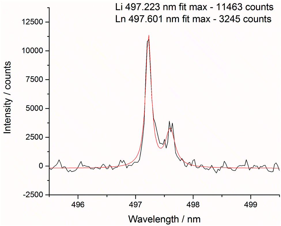 | ||
| Fig. 3 Lorentzian fit of normalisation peak (Li(I) 497.170 nm) and lanthanide element peak. | ||
To demonstrate the need for normalisation, charts of intensity at various emission peaks (for Er at 85 mJ per pulse) are shown below in Fig. 4. The upper chart shows the absolute intensity as recorded by the spectrometer, whereas the lower shows the intensity normalised against the Li line at 497.170 nm. Normalising the data leads to an observable increase in emission intensity with increasing concentration, in contrast to the absolute data which shows discrepancies away from this trend. The positive correlation of the normalised signal intensity to concentration resulted in improved modelling results.
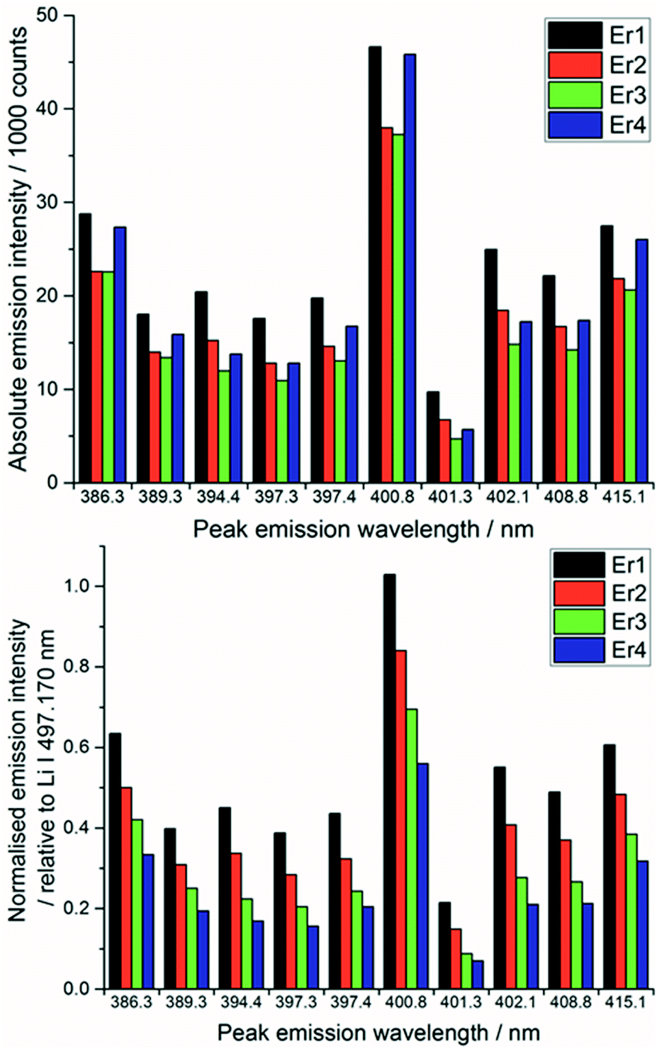 | ||
| Fig. 4 Comparison of Er emission line peak intensities with absolute intensity (above) and relative intensity (below) for four samples of erbium (Er1 = 0.158, Er2 = 0.076, Er3 = 0.039, Er 4 = 0.026 mmolEr gLKE−1). | ||
The Echelle spectrometer design generates an artificial intensity bias for wavelengths that fall in the centre of its pixel grid, meaning that across each order of the spectrometer there is an intensity maximum at the centre of that wavelength range. This artificially inflates the number of counts at certain periodic positions in each spectrum which increased the error of concentration models. This effect was particularly noticeable in the blank sample analyses. Since the Echelle orders are fixed at certain wavelength and pixel positions, a simple third-order fit of each order could be easily applied to all of the spectra in a dataset. To maintain the information contained in the spectral peaks whilst removing the artificial bias for the pixels at the centre of the camera grid, the fitted curve ignored vales above 1.5 times the mean for each region. One Echelle order of a blank sample is shown in Fig. 5, along with the third order fit and resulting corrected spectrum. All repeated measurements on the same sample were then averaged together.
 | ||
| Fig. 5 Example of Echelle order intensity bias between 332.8 and 339.2 nm (black – pre-treated spectrum; blue – third order fit; red – resulting treated spectrum). | ||
Applying a Savitzky–Golay filter to each spectrum was tested both before and after normalisation with various combinations of side points and polynomial orders. However, the signal quality was not noticeably improved, and the processing time for normalisation was increased from 0.1 second per spectrum to around 10 seconds per spectrum with the filter. The spectra were therefore analysed without any smoothing.
Using forward interval PLS (iPLS) (PLS Toolbox [Matlab]), predicted versus measured concentration models were plotted (using ‘leave-one-out’ cross validation) for each set of single lanthanide samples and for each of the three elements present in the mixed samples. An interval of 15 data points proved adequate to create accurate models for all of the analyses bar one (mixed lanthanide samples, Pr model), where the window was reduced to 5 points to improve the quality of the results.
Results and discussion
Preliminary experiments varying the laser pulse energy were carried out to identify the settings which maximised the signal to background ratio. After the best pulse energy and sampling techniques had been determined, further experiments were undertaken to analyse the full set of both single and mixed lanthanide samples for PLS concentration modelling.Fig. 6 shows an example spectral region of 385 to 391 nm and the high density of emission lines present. For the preliminary (laser pulse energy) experiments, the peak intensity data (from known emission lines) was used to ascertain the signal to background ratio, whereas for the concentration modelling experiments the whole spectrum was used for iPLS.
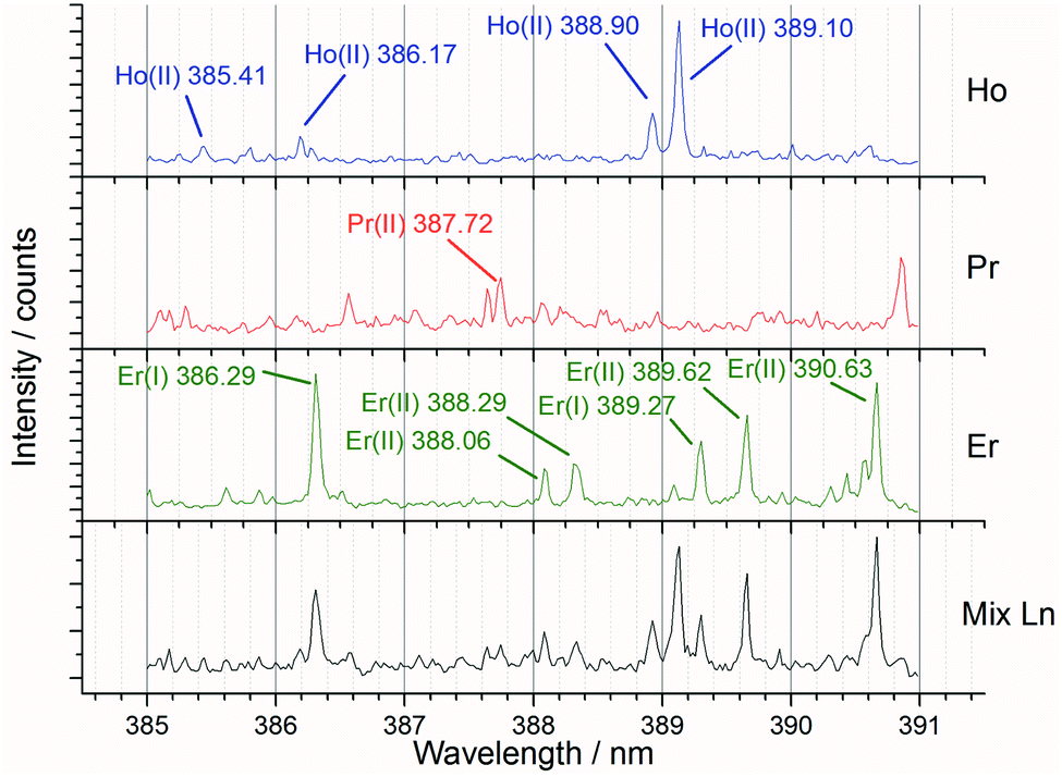 | ||
| Fig. 6 Annotated averaged LIBS spectra showing single lanthanide samples and a mixed lanthanide sample for the 385 to 391 nm window (recorded at 85 mJ per pulse). | ||
Laser pulse energy
The quality of LIBS spectra can be adversely affected by line broadening mechanisms which occur in the plasma, i.e. Doppler broadening and Stark broadening. Additionally, in this experiment, signal intensities changed markedly from shot to shot on the same spot of sample for both Li and lanthanide emission lines. We believe this may be because a relatively large amount of material was ablated by each laser shot, particularly at higher pulse energies, due to the relatively low density of the samples. Ablating greater amounts of sample from one spot lowered the height of the local sample surface and moved it out from the focal point of the laser radiation, thereby resulting in less material being ablated and thus reducing the emission intensity.15,32 Visual inspection of the samples indicated the ablation-craters were significantly larger for the higher pulse energies. Additionally, some of the ablation products were deposited on the sample chamber window, which reduced the power density at the sample surface.32,33 This effect was significantly worse at higher pulse energies, due to the increased amount of material ablated. The sample chamber window was cleaned after every experiment (i.e. every new sample or new pulse energy) to ensure the consistency of the analyses.The normalised spectral results, presented in Fig. 7, were obtained by using the ratio of lanthanide peak intensity to Li emission, and show a negative correlation between pulse energy and intensity, as indicated by the Pr1 emission. This is unexpected, as one would assume an equal ratio of Li and lanthanide are ablated with each shot on the same sample, independent of the total amount of material. It is possible that the Li peak chosen for normalisation was slightly affected by self-absorption, whereas the very intense 610 and 671 nm Li emissions showed obvious self-reversal, the 497.170 nm line did not appear to be affected. The changing pulse energy did not appear to have any effect on the RSD of the lanthanide emission intensity after normalisation against the lithium peak.
 | ||
| Fig. 7 Comparison of selected Pr emission line intensities at various pulse energies (average of 30 shots at each pulse energy). | ||
Principal Component Analysis (PCA) was used to further investigate the effect of pulse energy on the lanthanide emission spectra. The lanthanide emission peak-intensities were extracted from the averaged data for each single lanthanide sample at several pulse energies and used to construct PCA models. A full list of the emission peaks used is provided in Table 3. Fig. 8 shows highest concentration samples for Ho, Pr and Er measured at variable pulse energies (from 85 mJ per pulse up to 220 mJ per pulse). Each group of elements appears as an independent cluster. Additionally, the model is completely explained by three components (t[1] = 49%, t[2] = 40%, t[3] = 10%). For each of the three elements, the samples with the greatest separation were measured at the lowest pulse energy. Indeed, for each set of measurements there is a linear distribution emanating from the centre of the plot, with distance from the centre increasing with decreasing pulse energy.
| Species | λ/nm | Species | λ/nm | Species | λ/nm |
|---|---|---|---|---|---|
| Pr(II) | 381.602 | Ho(II) | 339.898 | Er(II) | 290.447 |
| Pr(II) | 387.718 | Ho(II) | 342.163 | Er(II) | 291.036 |
| Pr(II) | 396.481 | Ho(II) | 342.534 | Er(II) | 296.452 |
| Pr(II) | 399.479 | Ho(II) | 342.813 | Er(II) | 323.058 |
| Pr(II) | 400.869 | Ho(II) | 345.314 | Er(II) | 326.478 |
| Pr(II) | 405.488 | Ho(II) | 345.600 | Er(II) | 331.242 |
| Pr(II) | 405.654 | Ho(II) | 347.426 | Er(II) | 334.604 |
| Pr(II) | 406.281 | Ho(II) | 348.484 | Er(I) | 336.408 |
| Pr(II) | 410.072 | Ho(II) | 349.476 | Er(II) | 336.802 |
| Pr(II) | 411.846 | Ho(I) | 366.229 | Er(II) | 337.271 |
| Pr(II) | 414.122 | Ho(I) | 366.797 | Er(II) | 338.508 |
| Pr(II) | 414.311 | Ho(I) | 373.140 | Er(II) | 339.200 |
| Pr(II) | 416.416 | Ho(II) | 374.817 | Er(II) | 347.171 |
| Pr(II) | 417.939 | Ho(II) | 379.675 | Er(II) | 349.910 |
| Pr(II) | 418.948 | Ho(II) | 381.073 | Er(I) | 355.802 |
| Pr(II) | 420.672 | Ho(II) | 385.407 | Er(II) | 355.990 |
| Pr(II) | 422.293 | Ho(II) | 386.168 | Er(II) | 359.983 |
| Pr(II) | 422.535 | Ho(II) | 388.896 | Er(II) | 360.490 |
| Pr(II) | 430.576 | Ho(II) | 389.102 | Er(II) | 361.656 |
| Pr(II) | 436.833 | Ho(II) | 395.573 | Er(II) | 369.265 |
| Pr(II) | 440.882 | Ho(II) | 395.968 | Er(I) | 381.033 |
| Pr(II) | 442.925 | Ho(I) | 404.081 | Er(II) | 383.048 |
| Pr(II) | 444.983 | Ho(II) | 404.544 | Er(I) | 386.285 |
| Pr(II) | 446.866 | Ho(I) | 405.393 | Er(II) | 388.061 |
| Pr(II) | 449.646 | Ho(I) | 410.384 | Er(II) | 388.289 |
| Pr(I) | 468.780 | Ho(I) | 410.862 | Er(I) | 389.268 |
| Pr(I) | 469.577 | Ho(I) | 412.020 | Er(II) | 389.623 |
| Pr(II) | 473.669 | Ho(I) | 412.565 | Er(II) | 390.631 |
| Pr(I) | 490.699 | Ho(I) | 412.716 | Er(II) | 393.863 |
| Pr(I) | 491.402 | Ho(I) | 413.622 | Er(I) | 394.442 |
| Pr(I) | 492.460 | Ho(I) | 416.303 | Er(I) | 397.304 |
| Pr(I) | 493.600 | Ho(I) | 417.323 | Er(I) | 397.358 |
| Pr(I) | 494.030 | Ho(I) | 419.435 | Er(I) | 400.796 |
| Pr(I) | 495.137 | Ho(I) | 422.704 | Er(I) | 401.258 |
| Pr(I) | 501.859 | Ho(I) | 425.443 | Er(I) | 402.051 |
| Pr(I) | 501.976 | Ho(I) | 426.405 | Er(I) | 408.763 |
| Pr(I) | 502.696 | Ho(I) | 435.073 | Er(I) | 415.111 |
| Pr(I) | 504.383 | Ho(I) | 493.901 | ||
| Pr(I) | 504.552 | Ho(I) | 598.290 | ||
| Pr(I) | 505.340 | ||||
| Pr(I) | 508.712 | ||||
| Pr(I) | 513.344 | ||||
| Pr(II) | 525.973 |
 | ||
Fig. 8 Score scatter plot of PCA using highest-concentration single lanthanide samples at various pulse energies (540 V = 85 mJ per pulse; 560 V = 119 mJ per pulse; 580 V = 153 mJ per pulse; 600 V = 186 mJ per pulse; 620 V = 220 mJ per pulse). Ho – blue  , Pr – red , Pr – red  , Er – green , Er – green  (x axis component 1 = 49% explained, y axis component 2 = 40% explained). (x axis component 1 = 49% explained, y axis component 2 = 40% explained). | ||
As a result of the lowest pulse energy giving the greatest separation of samples, an additional PCA was carried out using only the lowest pulse energy measurements for each of the single lanthanide samples. The scores plot of this PCA is shown in Fig. 9. As with Fig. 8, there is a clear separation of sample groups into three independent clusters. Within each of these clusters, the highest concentration samples are further from the origin than the lower concentrations. Additionally, the three principal components completely explain the 3 groups of data (R2X cumulative = 99.2%). The near-linear spread of samples according to their concentration in this plot shows that multivariate analysis could be used to predict the concentration of lanthanide elements in a sample.
 | ||
Fig. 9 Score scatter plots using PCA analysis of peak intensity data for single lanthanide samples (pulse energy = 85 mJ per pulse). Upper figure: component 2 against component 1; lower figure: component 3 against component 1. Ho – blue  , Pr – red , Pr – red  , Er – green , Er – green  (component 1 = 47% explained, component 2 = 41% explained, component 3 = 12% explained). (component 1 = 47% explained, component 2 = 41% explained, component 3 = 12% explained). | ||
It was concluded that the lowest pulse energy gave the greatest normalised peak intensities and also the best separation of results in PCA modelling, whilst simultaneously damaging the sample less than higher pulse energies. On this basis the next set of experiments were conducted at the lowest possible pulse energy of 85 mJ per pulse. Additionally, only a single laser shot was used at each position to allow a repeatable sample surface for each measurement. Although this limited the number of measurements which could be obtained from each sample, it was deemed to be the best way of ensuring consistency.
Concentration prediction models
Forward iPLS is a technique used for variable selection in multivariate data analysis. The dataset is first split into a number of intervals, decided by the window size, and each of these is modelled using PLS. The model which returns the lowest Root Mean Square Error (RMSE) is identified. Next, this model is used in conjunction with the model of every other interval to try and improve the RMSE. Should a set of models reduce the RMSE, then this interval is added to the variable selection. This method is repeated until the error cannot be improved by the addition of any other model, at which point the variables identified are used to model the whole dataset. Complex datasets, such as those containing multiple species, are more likely to require a small window size so peaks from different species are not included in the same interval.Predicted versus measured concentration plots were constructed using forward iPLS with a window-size of 15 points. The plots are presented in Fig. 10 (a) (single element samples) and (b) (mixed lanthanide samples) and the figures of merit are summarised in Table 4. The overall linearity of the models is promising. Using a window-size of 15 points returned excellent RMSECV results for all of the single lanthanide samples and marginally higher (poorer) results for the mixed samples (as can be expected from the increased density of emission lines). The model for Pr in the mixed samples is the obvious outlier, with a significantly worse R2 value than the other plots. In order to improve the accuracy of this model the window size was reduced to 5 points, which increased the R2 value to be comparable with the other mixed lanthanide samples. However, this required an increase of the processing time from 10 seconds to 5 minutes.
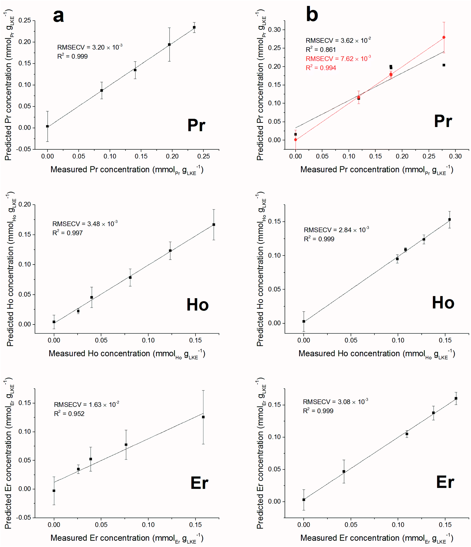 | ||
| Fig. 10 Predicted against measured concentrations for (a) single lanthanide samples and (b) mixed lanthanide samples (RMSECV given in units of mmolLn gLKE−1). Note different plots for (b) Pr: black line uses window of 15 points whereas red line uses window of 5 points to increase the model accuracy. | ||
| Model name | Latent variables | RMSECV (mmolLn gLKE−1) | R 2 | LoD (mmolLn gLKE−1) | LoQ (mmolLn gLKE−1) | LoD (ppm) | LoQ (ppm) |
|---|---|---|---|---|---|---|---|
| a w gives window size for mix Pr samples. | |||||||
| Pr | 3 | 3.20 × 10⁻³ | 0.999 | 0.0097 | 0.0322 | 541 | 1800 |
| Ho | 5 | 3.48 × 10⁻³ | 0.997 | 0.0115 | 0.0384 | 644 | 2150 |
| Er | 3 | 1.63 × 10⁻² | 0.952 | 0.0478 | 0.1593 | 2670 | 8900 |
| Mix Pr (w = 15)a | 4 | 3.62 × 10⁻² | 0.861 | 0.1423 | 0.4744 | 7960 | 26![[thin space (1/6-em)]](https://www.rsc.org/images/entities/char_2009.gif) 500 500 |
| Mix Pr (w = 5)a | 4 | 7.62 × 10⁻³ | 0.994 | 0.0054 | 0.0179 | 300 | 1000 |
| Mix Ho | 3 | 2.84 × 10⁻³ | 0.999 | 0.0077 | 0.0256 | 429 | 1430 |
| Mix Er | 4 | 3.08 × 10⁻³ | 0.999 | 0.0088 | 0.0294 | 494 | 1650 |
Limits of Detection (LoD) and Limits of Quantification (LoQ), shown in Table 4, for the single and the mixed lanthanide samples were calculated using ((1), (2) and (3)), where S is the standard error of regression, yi–ŷi is the distance between each data point and the linear calibration line, m is the gradient of the linear calibration line and df is the degrees of freedom of the model.
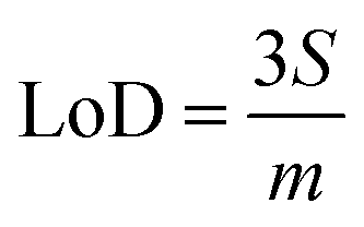 | (1) |
 | (2) |
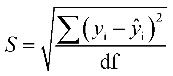 | (3) |
LIBS has traditionally suffered from higher LoD than other analytical techniques (e.g. TIMS, XPS etc.) due to the complex nature of interactions between the laser radiation, sample, plasma and surrounding atmosphere. However, the LoQ values here are below the concentrations that are likely to be encountered in industrial pyroprocessing facilities of spent nuclear fuel.
The Root Mean Square Error of Cross Validation (RMSECV) is another means to quantify the accuracy of a prediction of a PLS model. It is calculated with the average distance between values of predicted and actual lanthanide concentration using (4) (N is the number of points used to plot each graph). RMS Error of Prediction (RMSEP) is a similar measure but uses an external prediction set for validation.
 | (4) |
The LoD values calculated could be more accurate if samples of much higher concentration of lanthanide were used, as these would provide a better idea on linearity. However, the experiment was designed to simulate the intended industrial application, so the very low dilution of Ln elements is justified.
Interestingly, some of the regions selected by the iPLS software did not appear to contain any lanthanide emission lines. Using the Ho models for single and mixed lanthanide samples as an example, the single-lanthanide Ho iPLS selected only two regions to construct a model: 369.12–369.40 nm and 451.94–452.29 nm. The NIST atomic spectra database18 shows that former of these contains one Ho emission line at 369.195 nm, but the latter region does not contain any known Ho emission lines. Both intervals also are shown to contain Ar lines which may have played a role in the selection, although an Ar atmosphere was used in every measurement so should be irrelevant to the quantification process. In the case of the mixed-lanthanide Ho model, three regions were selected by the iPLS: 304.24–304.46 nm, 322.72–322.97 nm and 361.36–361.63 nm. The first two of these intervals do not contain any Ho emission lines according to the NIST database. The final interval does contain one Ho line at 361.331 nm (adjusting for spectrometer calibration error of up to +40 pm) and this peak can be seen on the spectrum. It is possible that the wide Lorentzian tails of nearby peaks have overlapped into the selected regions. Also, it may be that there are unreported Ho peaks, which is not uncommon for heavy elements with complex electronic structures such as the lanthanide or actinide series. A different way to validate the created models is to use an additional dataset as a prediction set. It is possible to use the single lanthanide samples as a prediction set for the mixed lanthanide models and vice versa. Fig. 11 shows the averaged Ho dataset (five samples plus blank) used as a prediction set for the mixed Ho model. Standard error of regression and R2 values are worse than for the models created with only either single or mixed samples. However, there is still a positive correlation between the prediction and measured concentration, which is good considering there were two other elements present in the calibration set. This information can be used to demonstrate the validity of the iPLS method and, in particular, the intervals selected by the PLS Toolbox software.
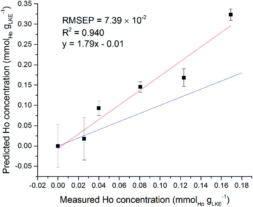 | ||
| Fig. 11 Ho single lanthanide samples as prediction set for Ho mixed lanthanide model. Red line is best fit of data points, blue line is ideal fit of y = x (RMSEP = 7.39 × 10⁻² mmolLn gLKE−1). | ||
Repeatability of measurements was an issue throughout the experiments. Some of the samples had clearly deteriorated in quality as a result of exposure to moisture as LKE is hygroscopic. This caused the samples to increase in diameter, resulting in an uneven sample surface. It is widely reported that LIBS analysis is particularly sensitive to sample-surface inhomogeneity.26 The differences in sample diameter were accounted for by adjusting the height of the stage (with respect to the laser focal point) for each measurement, but it was impossible to account for the variations in surface finish between the glassy and rough salt surfaces. It is worth noting, however, that in an industrial setting the sample would be a molten salt solution. Liquid samples provide a naturally level, even and self-healing surface, so the surface finish would be less of an issue (although other handling and experimental complications are associated with liquid-samples and LIBS17,31). Future experiments using molten salts could be accomplished with only minor changes to the experimental setup to allow this theory to be tested.
As an example of sample inhomogeneity, an iPLS model was created using only six spectra from each Ho sample plus the blank. This analysis used the venetian blinds cross-validation method34 with a window width of six to prevent falling into the sample replicate trap, and the predicted versus measured Ho concentration is shown in Fig. 12. There is a large variation in predicted concentrations for samples at the same measured concentration. There is an obvious need for brute force averaging of several repeat measurements before modelling or prediction. This is despite the spectral corrections such as normalisation and baseline-subtraction which have been detailed previously. The laser repetition rate limits the frequency of sampling in LIBS measurements. In our setup the repetition rate was 10 Hz. A similar system in an industrial setting (with more sample material) could record hundreds of repeat measurements in a matter of seconds and rapidly fulfil the need for averaging numerous spectra.
 | ||
| Fig. 12 Predicted vs. measured concentration of Ho samples. Model created using six individual spectra at each sample concentration rather than an average of all spectra at each sample concentration (RMSECV = 1.72 × 10⁻² mmolLn gLKE−1). | ||
Conclusions
The potential for concentration-prediction using LIBS has been demonstrated for lanthanide elements. Different concentrations of Ho, Er and Pr dissolved into LKE matrices were measured within an air-tight sample cell with a quartz viewing-window. Each LIBS emission spectrum was individually normalised with respect to a Li matrix peak at 497.170 nm and the Echelle-order baseline was subtracted (using a third-order plot of each Echelle-order wavelength range), before repeat measurements on the same sample were averaged together.Preliminary experiments investigating the laser pulse energy showed normalised lanthanide emission signal to noise ratio was improved at lower pulse energies. This was confirmed using PCA, which gave a better separation of samples recorded at the lowest pulse energies on a scores scatter plot.
Forward iPLS regression was used to construct concentration models for single lanthanide samples and for each of the three elements within mixed lanthanide samples. Using these models, predicted versus measured concentration graphs were plotted and used to estimate RMSECV, LoD and LoQ values. A standard window size of 15 points was used for iPLS across all the samples bar one, where it was necessary to reduce the window size to increase the accuracy. Some of the windows selected for incorporation into a model were shown to not contain any reported lanthanide emission lines. However, despite this, excellent RMSECV, Lod and LoQ values were obtained for all of the samples.
The PLS results suggest that LIBS could become a useful technique for the online monitoring of molten salt during pyroprocessing – particularly if deployment to an industrial setting could be validated by analysing molten samples or different matrix-salts. Additional improvements could be found by altering the ICCD camera settings (such as gate delay time and width) or investigating double-pulsed LIBS to maximise the signal to background ratio.
Conflicts of interest
There are no conflicts to declare.Acknowledgements
The Authors would like to thank the Atomic Weapons Establishment (AWE plc) and the Materials for Demanding Environments Centre for Doctoral Training (M4DE CDT) for funding of the PhD research project, and AWE for the loan of the LIBS apparatus.References
- T. Koyama, Y. Sakamura, M. Iizuka, T. Kato, T. Murakami and J.-P. Glatz, Procedia Chem., 2012, 7, 772–778 CrossRef CAS.
- R. Malmbeck, C. Nourry, M. Ougier, P. Souček, J. P. Glatz, T. Kato and T. Koyama, Energy Procedia, 2011, 7, 93–102 CrossRef CAS.
- H. Lee, G. Il Park, K. H. Kang, J. M. Hur, J. G. Kim, D. H. Ahn, Y. Z. Cho and E. H. Kim, Nucl. Eng. Technol., 2011, 43, 317–328 CrossRef CAS.
- IAEA, Assessment of Partitioning Processes for Transmutation of Actinides, Vienna, Austria, 2010 Search PubMed.
- J. J. Laidler, J. E. Battles, W. E. Miller, J. P. Ackerman and E. L. Carls, Prog. Nucl. Energy, 1997, 31, 131–140 CrossRef CAS.
- A. V. Bychkov, S. K. Vavilov, P. T. Porodnov, O. V. Skiba, G. P. Popkov and A. K. Pravdin, in Molten Salt Forum: Proceedings of the International Symposium on Molten Salt Chemistry and Technology 1998, ed. H. Wendt, Uetikon-Zuerich, Switzerland, 1998, pp. 525–528 Search PubMed.
- Y. Sakamura, T. Murakami, K. Tada and S. Kitawaki, J. Nucl. Mater., 2018, 502, 270–275 CrossRef CAS.
- J. Zhang, J. Nucl. Mater., 2014, 447, 271–284 CrossRef CAS.
- J. H. Yoo, C. S. Seo, E. H. Kim and H. S. Lee, Nucl. Eng. Technol., 2008, 40, 581–592 CrossRef CAS.
- C. A. Schroll, A. M. Lines, W. R. Heineman and S. A. Bryan, Anal. Methods, 2016, 8, 7731–7738 RSC.
- A. Lang, D. Engelberg, N. T. Smith, D. Trivedi, O. Horsfall, A. Banford, P. A. Martin, P. Coffey, W. R. Bower, C. Walther, M. Weiß, H. Bosco, A. Jenkins and G. T. W. Law, J. Hazard. Mater., 2018, 345, 114–122 CrossRef CAS.
- J. Wu, Y. Qiu, X. Li, H. Yu, Z. Zhang and A. Qiu, J. Phys. D: Appl. Phys., 2020, 53, 023001 CrossRef CAS.
- G. Maddaluno, S. Almaviva, L. Caneve, F. Colao, V. Lazic, L. Laguardia, P. Gasior and M. Kubkowska, Nucl. Mater. Energy, 2019, 18, 208–211 CrossRef.
- G. S. Maurya, A. Marín-Roldán, P. Veis, A. K. Pathak and P. Sen, J. Nucl. Mater., 2020, 541, 152417 CrossRef CAS.
- A. Williams, K. Bryce and S. Phongikaroon, Appl. Spectrosc., 2017, 71, 2302–2312 CrossRef CAS.
- M. Z. Martin, R. C. Martin, S. Allman, D. Brice, A. Wymore and N. Andre, Spectrochim. Acta, Part B, 2015, 114, 65–73 CrossRef CAS.
- A. Weisberg, R. E. Lakis, M. F. Simpson, L. Horowitz and J. Craparo, Appl. Spectrosc., 2014, 68, 937–948 CrossRef CAS.
- A. Kramida, Y. Ralchenko, J. Reader and The NIST ASD Team (2018), NIST Atomic Spectra Database, http://physics.nist.gov/asd%0Ahttps://doi.org/10.18434/T4W30F, accessed 15 January 2020 Search PubMed.
- X. Wang, V. Motto-Ros, G. Panczer, D. De Ligny, J. Yu, J. M. Benoit, J. L. Dussossoy and S. Peuget, Spectrochim. Acta, Part B, 2013, 87, 139–146 CrossRef CAS.
- V. K. Unnikrishnan, R. Nayak, P. Devangad, M. M. Tamboli, C. Santhosh, G. A. Kumar and D. K. Sardar, Mater. Lett., 2013, 107, 322–324 CrossRef CAS.
- B. T. Manard, E. M. Wylie and S. P. Willson, Appl. Spectrosc., 2018, 72, 1653–1660 CrossRef CAS.
- P. Devangad, V. K. Unnikrishnan, R. Nayak, M. M. Tamboli, K. M. Muhammed Shameem, C. Santhosh, G. A. Kumar and D. K. Sardar, Opt. Mater., 2016, 52, 32–37 CrossRef CAS.
- B. Bhatt, A. Dehayem-Kamadjeu and K. H. Angeyo, AIP Conf. Proc., 2019, 060006 CrossRef.
- P. Fichet, D. Menut, R. Brennetot, E. Vors and A. Rivoallan, Appl. Opt., 2003, 42, 6029 CrossRef CAS.
- J. R. Wachter and D. A. Cremers, Appl. Spectrosc., 1987, 41, 1042–1048 CrossRef CAS.
- C. Hanson, S. Phongikaroon and J. R. Scott, Spectrochim. Acta, Part B, 2014, 97, 79–85 CrossRef CAS.
- J.-I. Yun, R. Klenze and J.-I. Kim, Appl. Spectrosc., 2002, 56, 437–448 CrossRef CAS.
- J.-I. Yun, R. Klenze and J.-I. Kim, Appl. Spectrosc., 2002, 56, 852–858 CrossRef CAS.
- H. Hotokezaka, S. Tanaka, A. Suzuki and S. Nagasaki, Radiochim. Acta, 2000, 88, 645–648 CAS.
- N. A. Smith, J. A. Savina and M. A. Williamson, in Symposium on International Safeguards: Linking Strategy, Implementation and People, Vienna, Austria, 2014, pp. 1–7 Search PubMed.
- A. N. Williams and S. Phongikaroon, Appl. Spectrosc., 2017, 71, 744–749 CrossRef CAS.
- A. Williams and S. Phongikaroon, Appl. Spectrosc., 2018, 72, 1029–1039 CrossRef CAS.
- B. Yoo, S. H. Kim and J. Lee, in GLOBAL: Nuclear Fuel Cycle for a Low-Carbon Future, Paris, France, 2015, pp. 20–24 Search PubMed.
- D. Ballabio and V. Consonni, Anal. Methods, 2013, 5, 3790–3798 RSC.
Footnote |
| † UK Ministry of Defence © Crown Owned Copyright 2020/AWE |
| This journal is © The Royal Society of Chemistry 2021 |