
 Open Access Article
 This Open Access Article is licensed under a
 Creative Commons Attribution 3.0 Unported Licence
Synthesis of covalent organic frameworks using sustainable solvents and machine learning†
Sushil
Kumar
 ,
Gergo
Ignacz
and
Gyorgy
Szekely
*
,
Gergo
Ignacz
and
Gyorgy
Szekely
*
Advanced Membranes and Porous Materials Center, Physical Science and Engineering Division (PSE), King Abdullah University of Science and Technology (KAUST), Thuwal 23955-6900, Saudi Arabia. E-mail: gyorgy.szekely@kaust.edu.sa; Tel: +966128082769 Web: http://www.szekelygroup.com
First published on 8th October 2021
Abstract
Covalent organic frameworks (COFs) have attracted considerable interest owing to their structural predesign ability, controllable chemistry, long-range periodicity, and pore interior functionalization ability. The most widely adopted solvothermal synthesis of COFs requires the use of toxic organic solvents. In line with the 5th principle of green chemistry and the United Nations’ 12th Sustainable Development Goal, we aim to mitigate the adverse effect of solvents on COF synthesis. Here we have investigated twelve green solvents for the sustainable synthesis of five series of COFs using the solvothermal approach. Crystallinity and porosity were used to assess the quality of the obtained COFs. In addition, the suitability of the solvents in the synthesis of crystalline and porous COFs was investigated and color-coded for the final green assessment. In particular, γ-butyrolactone (for TpPa, TpBD, and TpAzo), para-cymene (TpAnq), and PolarClean (TpTab) were found to be excellent green solvents to produce high-quality COFs. For the first time, we successfully used quantitative structure–property relationships in combination with machine learning approaches to predict both the surface area and crystallinity of COFs using the structure of the solvents and COF building blocks.
Introduction
Two-dimensional (2D) covalent organic frameworks (COFs) have gained both academic and industrial interest owing to their unique design, ordered network, pore engineering, high porosity, and crystallinity.1,2 The conventional synthesis of long-range ordered COFs involves the formation of transposable connectivity through covalent bonds between symmetric organic building blocks in a symmetrical fashion. Consequently, COFs exhibit structural uniformity, periodicity, porosity, crystallinity, and framework robustness. Owing to these unique structural properties, the range of application of COFs is vast, including gas storage, separation, heterogeneous catalysis, energy storage and separation, supercapacitors and batteries, sensing, drug delivery, and optoelectronics.1,2In the past few years, we have witnessed a significant development in synthetic methods for the preparation of highly porous and long-range ordered COFs. The methods include solvothermal synthesis, mechanochemical grinding,3,4 ionothermal synthesis,5 microwave-assisted synthesis,6 interfacial polymerization,7,8 and microfluidic synthesis.9 Among these methods, the solvothermal approach has been widely used in the construction of high-quality COFs.10 This approach relies on solvent selection for reaction media. In particular, the nature of solvent, the solubility of precursors, temperature, and the duration of the reaction are considered as crucial factors, which affect the crystallinity and porosity of the resultant COFs. The solvothermal preparation of COFs often requires a combination of two organic solvents (e.g., mesitylene–dioxane) in a particular ratio. This method is not applicable for all types of COFs. Moreover, solvent mixtures are more difficult to recover and recycle, and therefore undesired from a green chemistry perspective.
The synthesis of newly designed COFs requires a cumbersome screening of organic solvents and their mixtures. The limited solubility of the precursors and their rate of diffusion in the selected solvent system significantly affect the crystallization process and ultimately, the quality of the obtained COFs. Therefore, understanding the structure–property relationship of the solvent–precursor nexus is crucial in the synthesis of high-quality COFs. The reaction medium has substantial contribution to the sustainability of synthetic processes.11 The application of green solvents in the solvothermal synthesis of COFs is scarce. Banerjee and co-workers successfully synthesized COFs in water using the dynamic covalent chemistry approach.12 Water is considered as an environmentally friendly reaction medium. The resulting COFs are porous and crystalline in nature. COFs with high surface areas were successfully prepared in ethanol, which is considered a green solvent.13,14 Deep eutectic solvents as green media for the synthesis of 2D and three-dimensional (3D) COFs based on Schiff-base chemistry were also reported. However, the porosity and crystallinity of the prepared COFs were compromised.15
Identification of efficient green solvents in the synthesis of COFs is a tedious task that is commonly performed via trial-and-error experimentation. However, the quantitative structure–property relationship (QSPR) tool, which is an emerging technique among the major computational methods in modern molecule design, could offer a resource and time efficient solution.16 QSPR analysis refers to any practical approach by which the chemical structure is quantitatively correlated with the physicochemical properties of the molecule or material. QSPR models have already found application in assessing the potential impacts of chemicals and nanomaterials on both living and synthetic systems. There have been no QSPR or any related quantitative structural–activity relationship-based studies on the property prediction of COFs.
In this work, we surveyed various green solvents as reaction media for the synthesis of high-quality COFs. We prepared five series of β-ketoenamine-based COFs in twelve different green solvents (Fig. 1). We identified the best solvent for each series that is suitable to deliver highly porous and crystalline COFs. The QSPR was used to identify the key structural elements affecting the surface area and to determine if the resultant COFs are crystalline or amorphous by analysing the solvent–precursor pairs. We used the partial least squares (PLS) regression tool and 11 different machine learning (ML) algorithms for binary classification. Our study initiates the exploration of the field of COFs by design using advanced molecule design tools.
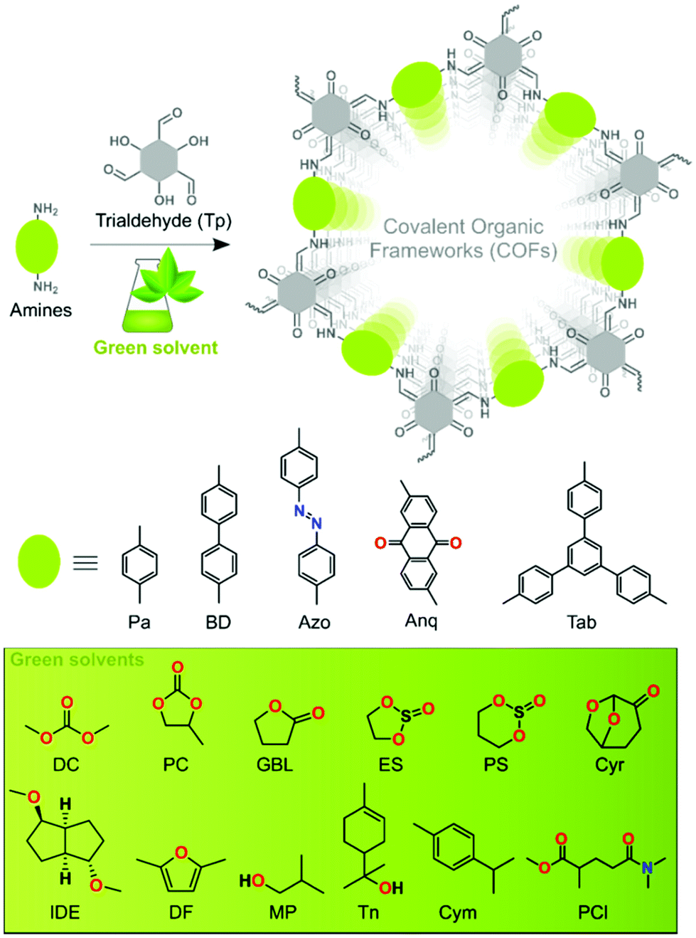 | ||
| Fig. 1 Schematic representation of COF synthesis using Tp trialdehyde and five different amines in green solvents. | ||
Experimental
COF synthesis
The solvothermal syntheses of five series of β-ketoenamine-based COFs were performed by employing twelve different bio-based green solvents such as dimethyl carbonate (DC), propylene carbonate (PC), γ-butyrolactone (GBL), 1,2-ethylene sulfite (ES), 1,3-propylene sulfite (PS), cyrene (Cyr), isosorbide dimethyl ether (IDE), 2,5-dimethyl furan (DF), 2-methyl-1-propanol (MP), terpineol (Tn), para-cymene (Cym), and Polar-Clean (PCl) (Fig. 1). A Pyrex tube was charged with 0.3 mmol Tp, 0.45 mmol of the corresponding diamines, i.e., 1,4-phenylenediamine (Pa), benzidine (BD), 4,4′-azodianiline (Azo), 2,6-diaminoanthraquinone (Anq), and 0.3 mmol of triamine, i.e., 1,3,5-tris(4-aminophenyl)benzene (Tab), and 3 mL of a green solvent having 0.2 mL of glacial acetic acid (3 M) as a green catalyst. After sonication for 15 min, the reaction mixture was subjected to three consecutive freeze–pump–thaw cycles under liquid nitrogen. The tube was sealed under 1 mbar vacuum and heated at 120 °C for 72 h in a preheated oven (section S2, ESI†). Prior to characterization studies, the resulting solid COF material was washed and dried at 90 °C under 1 mbar vacuum overnight.COF characterization
The crystallinities of the COFs prepared were determined from the powder X-ray diffraction (PXRD) patterns collected using a Bruker D8 ADVANCE with a high-intensity microfocus rotating anode X-ray generator. The PXRD patterns of the COFs were recorded in the 2θ range between 2.5° and 40°, and the data were obtained using the DIFFRACplus XRD Commander software. The radiation used was CuKα (α = 1.54 Å) with a Ni filter, and the data collection was performed using a Quartz holder at a scan speed of 1° min−1 and a step size of 0.01°. Fourier-transform infrared (FTIR) spectra were obtained using a Thermo Scientific Nicolet iS10 spectrometer with a universal Zn–Se attenuated total reflection accessory. Solid-state 13C cross polarization magic angle spinning (CP-MAS) NMR spectra were measured using a Bruker Avance III 400 MHz widebore instrument. Thermogravimetric analyses (TGA) were performed on a TGA 209 F1 analyser (Netzsch) under an N2 atmosphere at a heating rate of 10 °C min−1 within the temperature range of 30–900 °C. Scanning electron microscopy (SEM) measurements were performed using a Magellan FEI 400. The samples were prepared by casting a drop of COFs dispersed in propan-2-ol on a silicon wafer. To avoid charging during the SEM analyses, all the samples were coated with a 3 nm-thick layer of iridium using a Q150 T S sputter coater prior to the analyses. Nitrogen adsorption analyses were performed at 77 K using a liquid nitrogen bath on a Micromeritics ASAP 2420 BET instrument. All the samples were degassed for 12 h at 140 °C under vacuum prior to gas adsorption studies. The surface areas were evaluated using a Brunauer–Emmett–Teller (BET) model applied between P/Po values that fall in the range of 0.05–0.3 for the COFs. The pore size distributions were calculated using the non-localized density functional theory (NLDFT) method.Dataset generation
The dataset was generated using the chemical structures of the precursors and the solvents (section S1, ESI†). The results were transformed into a matrix of (60,1) for the surface area, yield, and crystallinity. Chemical descriptors corresponding to each experimental data point (precursor and solvent) were calculated by Mordred and RDKit packages using a Python script,17 and the NaN values were removed. A total of 1860 classical 1D, 2D, and 3D molecular descriptors18 were calculated from the amine precursors and solvents each. The majority of descriptors belonged to the autocorrelation, the Barysz matrix, electrotopological atomic state, different topological and MoRSE type descriptors. For a more comprehensive collection of different descriptor types, refer to section S1, ESI.† The final dataset was a matrix of (60![[thin space (1/6-em)]](https://www.rsc.org/images/entities/char_2009.gif) 2639) containing 158340 data points. The dataset was split into train and test sets, and subjected to data analysis, PLS regression, and classification. The reduced and clean dataset contained 2631 molecular descriptors. The amorphous COFs, including low yield and surface area, were omitted from the dataset for surface area prediction and only used for crystallinity binary classification. The descriptors containing non-float values (e.g., lists, NaN, or string values) were also removed.
2639) containing 158340 data points. The dataset was split into train and test sets, and subjected to data analysis, PLS regression, and classification. The reduced and clean dataset contained 2631 molecular descriptors. The amorphous COFs, including low yield and surface area, were omitted from the dataset for surface area prediction and only used for crystallinity binary classification. The descriptors containing non-float values (e.g., lists, NaN, or string values) were also removed.
QSPR and ML-based predictions
PLS prediction was made in PLS Toolbox (Eigenvector Research) under a MATLAB environment. For cross-validation, we used random samples with seven-fold cross-validation. Optimal parameter selection based on the global minimum of the root-mean-square error of cross-validation (RMSECV) auto-scaling was used to pre-process the dataset, and the outliers were removed by plotting the first two latent variables on a 95% confidence ellipse. Variable selection on projection (VIP) scoring was used to reveal the relative impact of each molecular descriptor on the surface area. Validation of the PLS results was performed using cross-validation, external validation, and Y-scrambling to reduce and eliminate possible overfitting.19 The data were split into 80:20 ratio of training and test datasets, respectively. The training root-mean-square error of calibration (RMSEC) and the RMSECV were recorded. The test dataset was used to quantify the goodness of the model by predicting the test data from the known descriptors.
Binary classification was used for the prediction of the crystallinity of the COFs. The dataset consisted of the same descriptors that were used in the PLS dataset. The binary outcome of the reaction was “1” if the reaction resulted in a crystalline COF, and “0” if the reaction did not occur or resulted in an amorphous COF or a polymer. The final dataset contained 60 binary-valued outcomes and descriptors. The binary classification problem was chosen over regression analysis for the reaction outcome due to the small dataset and the missing correlation between the surface area, crystallinity, and yield. The dataset was split into training and test datasets in an 85:15 ratio. It was necessary to perform principal component analysis (PCA) and Y-scrambling (Y-randomization) due to the high dimensionality and the small dataset, respectively.20 The algorithms employed were k-nearest neighbours, sigmoid support vector machine (SVM), radial basis function (RBF) SVM, polynomial SVM, decision tree, random forest, artificial neural network, adaptive boosting (AdaBoost), naïve Bayes, and quadratic classifier algorithms (section S1, ESI†). All Python calculations were performed on 100% sustainable Google Cloud Platform.21
Results and discussion
A Schiff-base condensation reaction was performed between Tp and the respective amines in various green solvents using the solvothermal approach, thereby affording TpPa, TpBD, TpAzo, TpAnq, and TpTab COFs (Fig. 1). All the COFs were synthesized under identical reaction conditions for all the green solvents investigated. The crystallinity of the COFs was determined from PXRD patterns (Fig. 2; section S4, ESI†). The high-intensity first peak observed at a 2θ lower than 5° can be attributed to the strong diffraction from the [100] planes, while the broad peak observed at a 2θ higher than 25° can be attributed to the diffraction from the [001] planes. The PXRD observations suggest the π–π stacking of the COF layers along the [001] plane. The experimental PXRD patterns of the COFs were found to match well with the PXRD patterns simulated for the eclipsed AA stacking model (section S5, ESI†) and are in good agreement with the results of previous studies.4 The relatively high intensities of the first peaks demonstrate the high crystallinity of the COFs.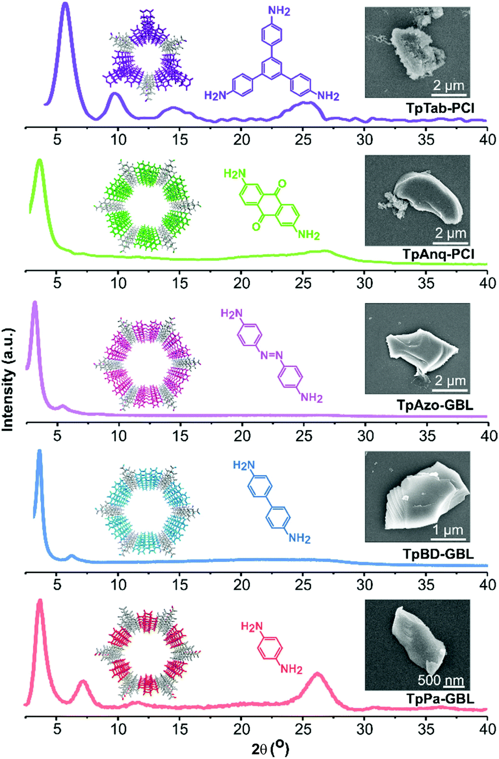 | ||
| Fig. 2 Examples of experimental PXRD patterns and SEM images of TpPa-GBL, TpBD-GBL, TpAzo-GBL, TpAnq-PCl, and TpTab-PCl COFs. | ||
The FTIR spectra of the COFs are in good agreement with those reported in the literature.4 The presence of strong peaks at 1250 cm−1 for ν(C–N) and 1575 cm−1 for ν(C![[double bond, length as m-dash]](https://www.rsc.org/images/entities/char_e001.gif) C) confirmed that the precursors, i.e., Tp and amines, were covalently linked together via the formation of β-ketoenamine moieties in the framework (section S6, ESI†). We have performed 13C CP-MAS solid-state NMR studies to explore the composition of the framework structure. The carbon signal present at approximately 180 ppm was assigned to the keto group, while the peak at 100 ppm corresponded to the CC bond adjacent to the keto group (section S7, ESI†).
C) confirmed that the precursors, i.e., Tp and amines, were covalently linked together via the formation of β-ketoenamine moieties in the framework (section S6, ESI†). We have performed 13C CP-MAS solid-state NMR studies to explore the composition of the framework structure. The carbon signal present at approximately 180 ppm was assigned to the keto group, while the peak at 100 ppm corresponded to the CC bond adjacent to the keto group (section S7, ESI†).
The chemical structure of the COFs was characterized using XPS profiles (section S8, ESI†). For example, the TpPa COF showed three intense peaks at 284.62, 399.63, and 530.62 eV, which correspond to C (1s), N (1s), and O (1s) signals, respectively. Detailed analysis of the high-resolution XPS profile is shown in Fig. S25, ESI.† The high-resolution profile for C (1s) displayed three main peaks and one additional π–π* satellite peak. The peak at 284.13 eV corresponded to the CC bond of the aromatic rings, where the shoulders at 285.36 and 287.01 eV were assigned to the C–O and CO bonds, respectively, present in the framework backbone. The high-resolution profile for N (1s) showed a peak at 399.63 eV, which corresponded to the C–NH moiety of the ketoenamine bond of the framework. In the high-resolution profile of O (1s), the peak signals that appeared at 530.49 and 532.21 eV were assigned to the CO and C–O bonds, respectively. For the detailed analysis of the XPS profiles, refer to section S8 in the ESI.† All the COFs exhibited good thermal stability up to approximately 350 °C (section S9, ESI†). The COFs displayed a sheet texture with lateral dimensions of 1–5 μm for all the COFs (section S10, ESI†).
The permanent porosity of the COFs was evaluated by measuring the nitrogen gas uptake at 77 K (section S12, ESI†). The obtained BET surface area (SABET) of the COFs spanned across a wide range of 30 to 1674 m2 g−1 depending on the green solvent employed (Fig. 3). Among all the COFs reported in this work, TpAzo-GBL exhibited the highest surface area of 1674 m2 g−1, followed by 1046 (TpBD-GBL), 1036 (TpTab-PCl), 1033 (TpAnq-Cym), and 888 (TpPa-GBL). Note that most of the COFs synthesized here exhibited improved surface area values as compared to the ones reported in conventional organic solvents.2 The pore size distributions for the as-synthesized COFs are presented in section S13 (ESI)† and were found to be approximately 15 Å (TpPa), 18 Å (TpBD), 22 Å (TpAzo), 18 Å (TpAnq), and 14 Å (TpTab), which were calculated on the basis of the NLDFT model.
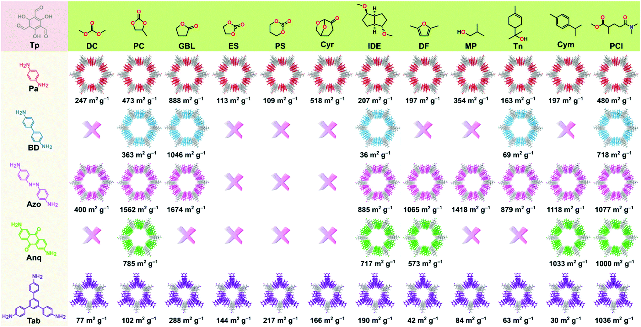 | ||
| Fig. 3 Forty-three COFs were synthesized in twelve different green solvents. Surface area values for each COF have been provided at the bottom of each COF structure. The cross sign signifies either no reaction or amorphous polymer formation. | ||
Fig. 1 shows the list of the green solvents used for the synthesis of the COFs. Solvents can be classified into seven classes: carbonates, esters, ethers, sulfites, alcohols, aromatic solvents, and aprotic solvents. A color-coding system was introduced in the GlaxoSmithKline and CHEM21 solvent selection guides,22–24 which were successfully used to describe the sustainable synthesis of UiO-66.25 We employed the same color-coding system in this work (section S14, ESI†). The column “overall green assessment”, which shows the color code for the green solvents utilized for the synthesis of the COFs, is based on the solvent greenness mentioned in the solvent selection guides (section S14, ESI†). The color codes for boiling point, viscosity, the presence of a characteristic PXRD peak (corresponds to diffraction from 100 planes), and SABET column are defined according to the ranges mentioned in Table S14, ESI.† The conventional solvents reported for the synthesis of COFs were also included as a reference for comparison.
The color codes for the last two columns define the rank by default and ranking after discussion. The column named as “rank by default” indicates the composite color extracted from the combined evaluation of solvent as well as the COF properties. Owing to the prime importance of the crystallinity and surface area of the COFs in a wide range of applications, the final color code in the “rank by default” column is dominated by the porosity of the COFs. Finally, the color code in the column “ranking after discussion” indicates the compatibility of the employed solvent and has been interpreted after an overall evaluation of solvent properties in the generation of crystalline and porous COFs. In general, the green code denotes efficient solvents with minor issues, the yellow code for solvents that can be used but are found to be less efficient, and the red code for solvents that are either not recommended (according to solvent selection guides) or resulted in very low crystalline porous COFs.
To assess the suitability of green solvents in the preparation of high-quality COFs, we calculated the relative SABET, relative crystallinity, and relative yield for the COFs. As shown in Fig. 4a, the TpPa, TpBD, and TpAzo COFs synthesized in GBL displayed high BET surface area values. In contrast, in the case of the TpAnq and TpTab COFs, the Cym and PCl solvents were found to be efficient in delivering highly porous COFs. In terms of the crystallinity of the COFs, the results were quite vague and the data points were scattered all over the plot (Fig. 4b). All the solvents afforded relatively moderate to low crystalline COFs. This suggests difficulty in correlating the crystallinity of the as-synthesized COFs with respect to the solvents used. A similar kind of observation was made with the relative yield plot (Fig. 4c); the data points were randomly distributed across the plot, making it difficult to directly correlate with the COFs synthesized in this study. For example, PC resulted in high yields for TpBD and TpAzo; however, it afforded moderate to low yields of other COFs. In other words, on the basis of relative crystallinity and yield, it is difficult to obscure a strong correlation of these COF properties with the solvents employed.
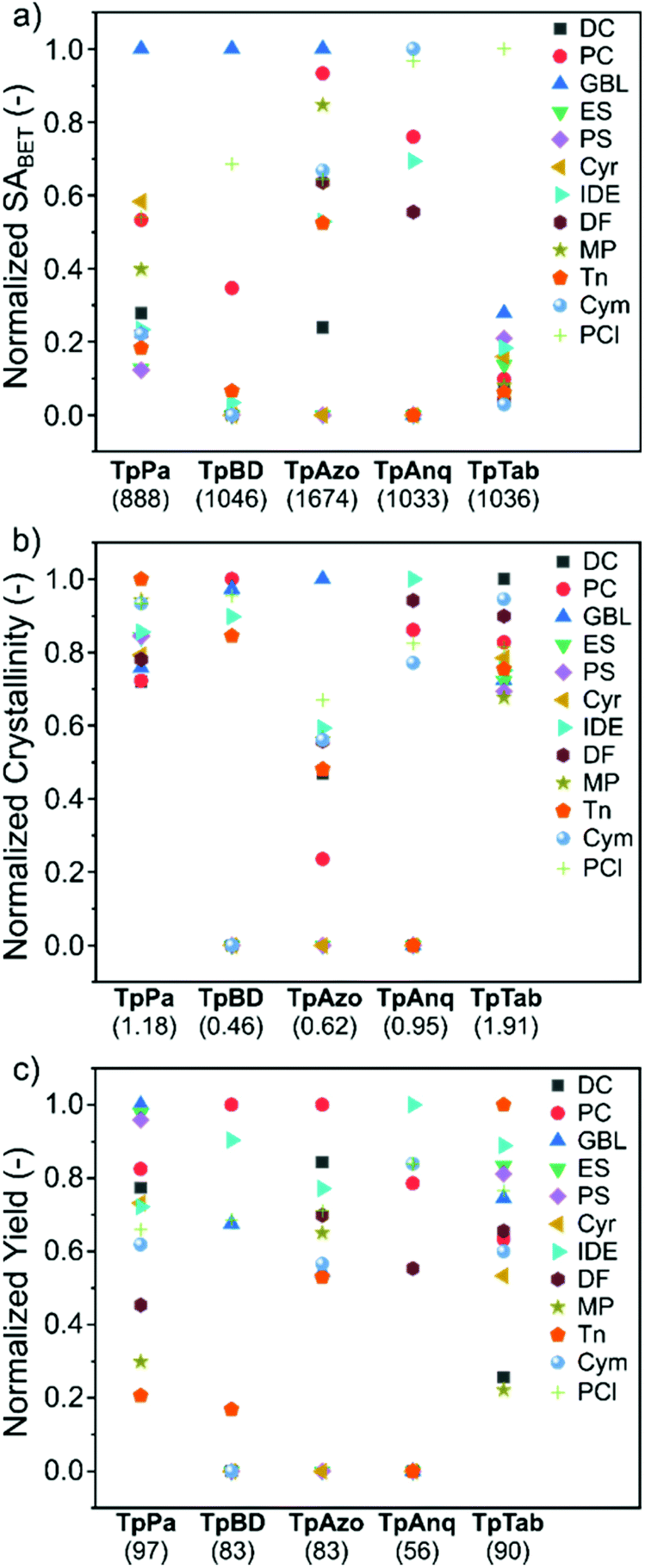 | ||
| Fig. 4 (a) Relative surface area, (b) relative crystallinity, and (c) relative yield of the TpPa, TpBD, TpAzo, TpAnq, and TpTab series of COFs synthesized in twelve green solvents. The value provided in parenthesis along the x-axis denotes the maximum value of (a) BET surface area (m2 g−1), (b) crystallinity, and (c) yield (%) used in the calculations (section S4, ESI†). | ||
To address this problem, for the very first time, we utilized an ML approach to deduce the structure–property relationship between the solvents and resultant COFs. The surface area of the COFs is co-dependent on the type of solvent(s) used. Thus, classical ab initio DFT calculations would require overly complex methods to quantify the properties of COFs.26 To overcome the issues with solvent dependency, we used QSPR computational tools to predict the surface area and to verify if the resultant COF can be synthesized in the crystalline form. We hypothesized that by determining the structure of the solvent and the structure of the COF, a predictive relationship could be drawn while other parameters can be kept constant. Using a dataset with 60 points with high-capacity ML and deep learning methods remains a challenge since they generally require a large amount of data to obtain good predictive results. Using the QSPR approach, we developed a quantitative structural–property relationship to predict the key structural elements necessary to generate high surface area and crystalline COFs by analyzing the solvent–amine precursor pairs. Initially, a cross-correlation analysis between the obtained results was necessary to filter out relationships across the surface area, crystallinity, and yield. No direct correlation for the highly scattered, randomly distributed points was observed for the yield-surface area results (Fig. S54a, ESI†). Similarly, the crystallinity-yield (Fig. S54b, ESI†) and the crystallinity-surface area (Fig. S54c, ESI†) datasets did not reveal any correlation. The non-correlated data indicate that, for example, a COF obtained in a high yield does not necessarily have a high surface area. Having no correlations across the results suggests that the surface area, crystallinity, and yield data need to be predicted separately; thus, none of them could be obtained one from the other.
With only 43 measured surface area data points and 2639 calculated descriptors (predictor features), the original dataset was high-dimensional and prone to suffer from dimensionality issues, making the application of classical prediction methods challenging.27 To overcome the issues related to high dimensionality datasets, PLS regression and PCA were applied to the dataset. PLS regression and PCA are useful when the number of predictor features is high, and they are possibly cross-correlated. Using a PLS model, the response features were predicted from a large set of predictor features by reducing the set of the latter to a smaller set of uncorrelated components (projection to latent structures). In the model-building phase, the original dataset contained a matrix of 3672 molecular descriptors of the used solvents and amine precursors as the X matrix, and the surface area and the binary results of the corresponding COF as Y variables as a vector. The first two PLS components were plotted against each other, and the outliers were removed based on a 95% confidence ellipse. The resultant matrix of (392631) was split and standardized.
The optimal number of PLS components was found to be 3 with seven-fold cross-validation and a blind thickness of 1 based on the average minimum of the RMSECV values. The RMSEC and RMSECV values were found to be 119 and 174 from the Y-scrambling test, respectively. In contrast, RMSEP was 199 based on the Y-scrambling test. The insignificant difference between the cross-validation and the test R2 score values indicates no overfitting. The prediction error agrees well with the measured general error of the surface area of the microporous materials.28Fig. 5 shows general model training and test data with the corresponding trend line. The error of the surface area was found to increase with an increase in the surface area. In general, the model shows a strong correlation between the predicted and measured surface area. Based on the VIP scoring, 196 descriptors were selected (refer to VIP scoring, section S15, ESI†) from descriptors with the highest VIP scoring related to the amine precursors’ and the solvents’ electronic structures. From the best 196 descriptors 90 of them were ligand descriptors (45%), which means that the BET surface area is dependent on the structure of both the solvent and the ligand. Interestingly, out of the top 50 descriptors, only 12 belonged to the ligands (24%), and the first ligand descriptor was only the 17th from the absolute value sorted PLS prediction list. The highest scoring descriptors belonged to hybridization factor, spatial autocorrelation values (Moran's index), electrotopological state indexes and the logP of the solvent. The highest scoring ligand descriptor was also a spatial autocorrelation index (electronegativity weighted Geary index). Fig. S1† shows the VIP scoring in decreasing absolute order. There was no single outstanding descriptor with several mid-range VIP scores, emphasizing the complexity in surface area prediction. For the captured variance values and model parameter diagram, refer to section S15 (ESI).† The crystallinity of the COFs depends on the PXRD measurement parameters, while yield results generally have a high error. Thus, the yield and crystallinity results were combined and simplified for use in the prediction. The binary classification problem was created by combining the yield and crystallinity results into simple crystalline COF/amorphous COF data. The original dataset contained a matrix of (602631) molecular descriptors of the used solvents and amine precursors as the X matrix and the binary values of crystalline/amorphous COFs as the Y vector. The results of the binary classification ML algorithms and classical statistical methods are shown in Fig. 5. The performance of the naïve Bayes and QDA algorithms was better than those of the SVM, decision tree, random forest, artificial neural network, and boosting algorithms. This difference can be attributed to the insufficient data when the ML algorithms tend to underperform the classical statistical methods. Both the naïve Bayes and QDA reached an accuracy score of 0.87. For details of each algorithm, refer to section S15, ESI.†
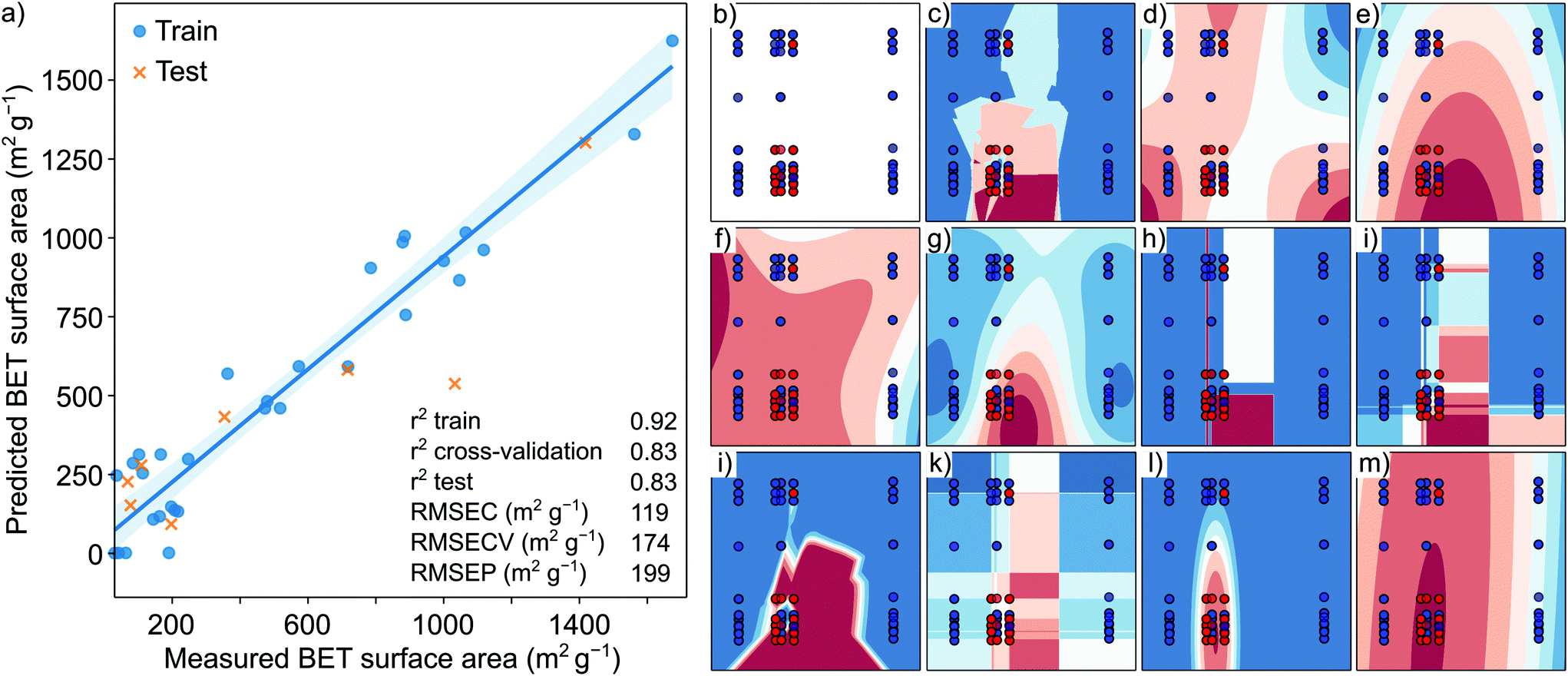 | ||
| Fig. 5 (a) Visualization of the predicted versus measured BET surface areas (m2 g−1). Visual representation of the binary classification results using different algorithms, where the accuracy score is provided in parenthesis: (b) input data projected on the principal component 1 (x-axis) and principal component 2 (y-axis), (c) k-nearest neighbor algorithm (0.83), (d) sigmoid support vector machine (0.70), (e) radial basis function support vector machine (0.71), (f) polynomial kernel support vector machine (0.71), (g) Gaussian process (0.82), (h) decision-tree algorithm (0.77), (i) random forest algorithm (0.73), (j) artificial neural network (shallow) (0.76), (k) adaptive boosting algorithm (0.79), (l) naïve Bayes method (0.87), and (m) quadratic statistical classifier (0.87). The higher the accuracy score, the higher the predictive power of the method. | ||
Real-world application
To test our model in a real-world application, we first used the best performing binary classification models (QDA and naïve Bayes) to predict the expected crystallinity of two new COFs in GBL and PCl solvents (Fig. 6). We chose these two solvents because, from the previous measurement, they yielded high surface area COFs. The two new COFs, namely TpPa2 and TpTta, were selected because the ligand amine is inherently different from that in the training set. Using diverse ligands, we further tested the robustness of the model. The Pa2 ligand contains two methyl groups at para position to each other, while Tta contains a 1,3,5-triazine group in its core. Note that in the training set, not a single ligand included either an aliphatic side group or a heteroaromatic core. The predicted surface area was 364 and 175 m2 g−1 for the TpPa2 COF in PCl and GBL, respectively. The predicted surface area was 963 and 774 m2 g−1 for the TpTta COF in PCl and GBL, respectively (Fig. 6). The TpPa2 and TpTta COFs were synthesized using the same solvothermal method described above. All four COFs were crystalline with moderately high yield and PXRD results (section S16, ESI†). The measured surface areas were in close agreement with the predictions. The RMSE was 124 for the predictions, lower than the test RMSE from the model building phase. We demonstrated that our ML-based methodology has excellent predictive power with respect to crystallinity and surface area of COFs, which could open new avenues for in silico COF design strategies.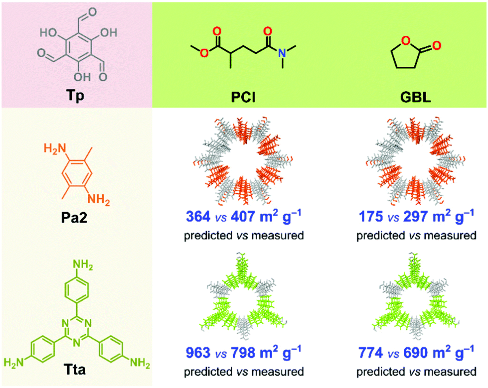 | ||
| Fig. 6 Comparison of predicted vs. measured SABET of two COFs synthesized in PCl and GBL solvents. | ||
Conclusions
We synthesized forty-three COFs, falling into five series, in twelve green solvents using an acetic acid green catalyst through a solvothermal method. The suitability of the green solvents in the synthesis of the high-quality COFs was investigated by correlating the relative surface area, crystallinity, and yield of the resultant COFs with varying parameters of the green solvents. The gas adsorption studies and PXRD patterns indicate the possible role of green solvents as reaction media in navigating the formation of high-quality COFs. Using ML approaches for the first time, we successfully demonstrated that the surface area of the COFs can be predicted using solvent and amine precursor descriptors with 0.83 R2 values in the PLS regression analysis. We also demonstrated that the formation of crystalline or amorphous COFs can be predicted using ML binary classification by only using the solvent media and the amine precursor's descriptors, achieving an accuracy score of 0.87. In future, we aim to design new ML experiments to identify a better correlation of the efficiency of the most promising solvent with high-quality COF preparation. We believe that these preliminary results will provide a fundamental understanding of solvent behavior and provide access to several other green solvents used in preparing high-performance COFs. The real-world application showed the robustness of the model, which can be extended to design new COFs. The binary classification model is an excellent tool to predict whether a COF can be synthesized in an amorphous or crystalline form, while the surface area predictions were similar to the measured values.Author contributions
Sushil Kumar: Investigation, validation, formal analysis, data curation, visualization, and writing—original draft. Gergo Ignacz: modeling, formal analysis, visualization, and writing—original draft. Gyorgy Szekely: conceptualization, methodology, resources, visualization, writing—review & editing, supervision, funding acquisition, and project administration.Conflicts of interest
There are no conflicts to declare.Acknowledgements
This work was supported by the King Abdullah University of Science and Technology (KAUST). The postdoctoral (SK) and PhD (GI) fellowships from the Advanced Membranes and Porous Materials Center at KAUST are gratefully acknowledged.References
- S. J. Lyle, P. J. Waller and O. M. Yaghi, Trends Chem., 2019, 1, 172–184 CrossRef CAS.
- K. Geng, T. He, R. Liu, S. Dalapati, K. T. Tan, Z. Li, S. Tao, Y. Gong, Q. Jiang and D. Jiang, Chem. Rev., 2020, 120, 8814–8933 CrossRef CAS PubMed.
- B. P. Biswal, S. Chandra, S. Kandambeth, B. Lukose, T. Heine and R. Banerjee, J. Am. Chem. Soc., 2013, 135, 5328–5331 CrossRef CAS PubMed.
- S. Karak, S. Kandambeth, B. P. Biswal, H. S. Sasmal, S. Kumar, P. Pachfule and R. Banerjee, J. Am. Chem. Soc., 2017, 139, 1856–1862 CrossRef CAS PubMed.
- P. Kuhn, M. Antonietti and A. Thomas, Angew. Chem., Int. Ed., 2008, 47, 3450–3453 CrossRef CAS PubMed.
- M. Dogru, A. Sonnauer, S. Zimdars, M. Döblinger, P. Knochel and T. Bein, CrystEngComm, 2013, 15, 1500–1502 RSC.
- K. Dey, M. Pal, K. C. Rout, S. Kunjattu H, A. Das, R. Mukherjee, U. K. Kharul and R. Banerjee, J. Am. Chem. Soc., 2017, 139, 13083–13091 CrossRef CAS PubMed.
- D. B. Shinde, G. Sheng, X. Li, M. Ostwal, A.-H. Emwas, K.-W. Huang and Z. Lai, J. Am. Chem. Soc., 2018, 140, 14342–14349 CrossRef CAS PubMed.
- D. Rodríguez-San-Miguel, A. Abrishamkar, J. A. R. Navarro, R. Rodriguez-Trujillo, D. B. Amabilino, R. Mas-Ballesté, F. Zamora and J. Puigmartí-Luis, Chem. Commun., 2016, 52, 9212–9215 RSC.
- P. J. Waller, F. Gándara and O. M. Yaghi, Acc. Chem. Res., 2015, 48, 3053–3063 CrossRef CAS PubMed.
- T. Welton, Proc. R. Soc. A, 2015, 471, 20150502 CrossRef PubMed.
- J. Thote, H. Barike Aiyappa, R. Rahul Kumar, S. Kandambeth, B. P. Biswal, D. Balaji Shinde, N. Chaki Roy and R. Banerjee, IUCrJ, 2016, 3, 402–407 CrossRef CAS PubMed.
- C.-X. Yang, C. Liu, Y.-M. Cao and X.-P. Yan, Chem. Commun., 2015, 51, 12254–12257 RSC.
- L. Cseri, M. Razali, P. Pogany and G. Szekely, Organic solvents in sustainable synthesis and engineering, ed. B. Török and T. B. T.-G. C. Dransfield, Elsevier, 2018, pp. 513–553 Search PubMed.
- J. Qiu, P. Guan, Y. Zhao, Z. Li, H. Wang and J. Wang, Green Chem., 2020, 22, 7537–7542 RSC.
- E. N. Muratov, J. Bajorath, R. P. Sheridan, I. V. Tetko, D. Filimonov, V. Poroikov, T. I. Oprea, I. I. Baskin, A. Varnek, A. Roitberg, O. Isayev, S. Curtalolo, D. Fourches, Y. Cohen, A. Aspuru-Guzik, D. A. Winkler, D. Agrafiotis, A. Cherkasov and A. Tropsha, Chem. Soc. Rev., 2020, 49, 3525–3564 RSC.
- H. Moriwaki, Y.-S. Tian, N. Kawashita and T. Takagi, J. Cheminf., 2018, 10, 4 Search PubMed.
- R. Todeschini and V. Consonni, Handbook of Molecular Descriptors, Wiley-VCH, 2000, vol. 11, p. 688 Search PubMed.
- P. Gramatica, QSAR Comb. Sci., 2007, 26, 694–701 CrossRef CAS.
- P. F. J. Lipiński and P. Szurmak, Chem. Pap., 2017, 71, 2217–2232 CrossRef PubMed.
- Carbon neutral since 2007. Carbon free by 2030., https://sustainability.google.
- R. K. Henderson, C. Jiménez-González, D. J. C. Constable, S. R. Alston, G. G. A. Inglis, G. Fisher, J. Sherwood, S. P. Binks and A. D. Curzons, Green Chem., 2011, 13, 854–862 RSC.
- C. M. Alder, J. D. Hayler, R. K. Henderson, A. M. Redman, L. Shukla, L. E. Shuster and H. F. Sneddon, Green Chem., 2016, 18, 3879–3890 RSC.
- D. Prat, A. Wells, J. Hayler, H. Sneddon, C. R. McElroy, S. Abou-Shehada and P. J. Dunn, Green Chem., 2016, 18, 288–296 RSC.
- D. Morelli Venturi, F. Campana, F. Marmottini, F. Costantino and L. Vaccaro, ACS Sustainable Chem. Eng., 2020, 8, 17154–17164 CrossRef CAS.
- A. Datar, Y. G. Chung and L.-C. Lin, J. Phys. Chem. Lett., 2020, 11, 5412–5417 CrossRef CAS PubMed.
- I. M. Johnstone and D. M. Titterington, Philos. Trans. R. Soc., A, 2009, 367, 4237–4253 CrossRef PubMed.
- P. Sinha, A. Datar, C. Jeong, X. Deng, Y. G. Chung and L.-C. Lin, J. Phys. Chem. C, 2019, 123, 20195–20209 CrossRef CAS.
Footnote |
| † Electronic supplementary information (ESI) available. See DOI: 10.1039/d1gc02796d |
| This journal is © The Royal Society of Chemistry 2021 |