 Open Access Article
 This Open Access Article is licensed under a Creative Commons Attribution-Non Commercial 3.0 Unported Licence
Introductory lecture: air quality in megacities
Luisa T.
Molina
 ab
ab
aMolina Center for Energy and the Environment, La Jolla, California 92037, USA. E-mail: ltmolina@mce2.org
bDepartment of Earth, Atmospheric and Planetary Sciences, Massachusetts Institute of Technology, Cambridge, Massachusetts 02139, USA. E-mail: ltmolina@mit.edu
First published on 30th October 2020
Abstract
Urbanization is an ongoing global phenomenon as more and more people are moving from rural to urban areas for better employment opportunities and a higher standard of living, leading to the growth of megacities, broadly defined as urban agglomeration with more than 10 million inhabitants. Intense activities in megacities induce high levels of air pollutants in the atmosphere that harm human health, cause regional haze and acid deposition, damage crops, influence air quality in regions far from the megacity sources, and contribute to climate change. Since the Great London Smog and the first recognized episode of Los Angeles photochemical smog seventy years ago, substantial progress has been made in improving the scientific understanding of air pollution and in developing emissions reduction technologies. However, much remains to be understood about the complex processes of atmospheric oxidation mechanisms; the formation and evolution of secondary particles, especially those containing organic species; and the influence of emerging emissions sources and changing climate on air quality and health. While air quality has substantially improved in megacities in developed regions and some in the developing regions, many still suffer from severe air pollution. Strong regional and international collaboration in data collection and assessment will be beneficial in strengthening the capacity. This article provides an overview of the sources of emissions in megacities, atmospheric physicochemical processes, air quality trends and management in a few megacities, and the impacts on health and climate. The challenges and opportunities facing megacities due to lockdown during the COVID-19 pandemic is also discussed.
Introduction
Megacities (metropolitan areas with populations over 10 million) present a major global environmental challenge. Rapid population growth, unsustainable urban development, and increased energy demand by transportation, industrial, commercial, and residential activities, have led to large amounts of emissions to the atmosphere that subject the residents to the health risks associated with harmful pollutants, and impose heavy economic and social costs. The dispersion of pollutants generated locally causes regional haze and acid deposition, damages crops and changes in the Earth’s radiative balance. Long-range transport of pollutants influences air quality in regions far from the megacity sources. However, as centers of economic growth, scientific advancement, technology innovation, and social and cultural activities, well-planned and densely populated urban centers can take advantage of the benefits of agglomeration by providing proximity to urban infrastructure and services and optimizing energy consumption, thus reducing atmospheric pollution and creating sustainable livable cities for the residents.1,2 This is especially critical as the phenomenon of urbanization continues in almost all countries across the world.In 1970, only 37% of the world’s population lived in urban areas; this increased to 55% by 2018 and is projected to increase to 68% by 2030, with almost 90% of the growth happening in Asia and Africa,3,4 as shown in Fig. 1. In 2018, about 23% of the world’s population lived in 550 cities with at least 1 million inhabitants, of which 50 cities had populations between 5 million and 10 million, and 33 cities had more than 10 million inhabitants (loosely defined as megacities). The world is projected to have 43 megacities (representing 8.8% of the global population of 8.5 billion) by 2030, with most of them located in developing countries,3 many are facing the challenge of growing their economies and managing the environment to provide better quality of life and cleaner and breathable air for the population.
 | ||
| Fig. 1 Evolution of megacities, showing percentage urban and urban agglomeration by size (adapted from the UN World Urbanization Prospect, 2018 revision).4 | ||
Activities from megacities are responsible for the emissions of primary pollutants, including gaseous species such as volatile organic compounds (VOCs), nitrogen oxides (NOx), carbon monoxide (CO), sulfur dioxide (SO2), ammonia (NH3) and air toxins (e.g., benzene, 1,3-butadiene), some of which contribute to the formation of secondary pollutants such as ozone (O3) and secondary aerosols; semi-volatile species (e.g., polycyclic aromatics, dioxins, furans); particulate matter (e.g., combustion soot, dust); and metals (e.g., lead, mercury). Despite the large amount of research that has been conducted, including air quality monitoring, field measurements and modeling studies, the sources and processes of emissions generated in megacities that lead to high concentrations of major pollutants such as ozone and secondary particulate matter, are still not well understood, thus limiting our ability to mitigate air pollution and make air quality forecasts to alert the residents of potentially unhealthy air pollution episodes.
This article will provide an overview on the sources of emissions in megacities, atmospheric physicochemical processes, air quality trends and management programs in a few megacities, and the impacts on health and climate change. The final section describes the challenges and opportunities facing the megacities due to lockdown during the COVID-19 pandemic. There is a very large volume of literature articles and topics related to megacities, this article will not be able to cover all of them, but will present the main ideas and include references where more information is available.
Sources of emissions in megacities
Emissions from megacities are caused by a wide variety of anthropogenic and natural sources. The major anthropogenic sources include: (i) mobile sources: on-road vehicles such as passenger cars, commercial buses and trucks, motorcycles and three-wheelers; non-road vehicles such as aircraft, marine vessels, construction and agricultural equipment; (ii) stationary sources such as factories, refineries, boilers and power plants; and (iii) area sources: small-scale industrial, commercial and service operations; municipal solid waste facilities/landfills and wastewater treatment plants; consumer products; residential heating/cooling and fuel use; construction activities; mining operations; agricultural activities and confined animal feeding operations. Natural (biogenic) sources include vegetation, windblown soils, volcanoes, lightning, forest and grassland fires, and sea salt spray.The following sections provide an overview of some of the major sources and control strategies.
Transportation
In many megacities and large urban centers around the world, emissions from the transportation sector are a major source of air pollution.1,2,5 The combustion of fossil fuels from mobile sources are responsible for large emissions of particulate matter composed of black carbon, organic carbon and other inorganic components, CO2, CO, NOx, VOCs and air toxics. The emissions contributions from mobile sources may vary widely among the megacities, depending on the technical characteristics of the vehicle fleet, the quality of the fuels consumed, the level of local development and intensity of economic activities, and the volume of vehicular travel.Several megacities have implemented measures to reduce emissions from on-road vehicles, including improvement of vehicle technology and fuel quality, implementation of strict international vehicle emission standards, replacement of diesel with natural gas, and introduction of hybrid and electric vehicles. Some megacities have introduced more efficient mobility through a number of strategies, such as improving the efficiency and security of the public transportation network to encourage use of public transit, expanding infrastructure for non-motorized transportation (walking and cycling); reducing traffic congestion by limiting the circulation of vehicles (e.g., “No drive day” in Mexico and many megacities) (SEDEMA, http://www.aire.cdmx.gob.mx) and road pricing (e.g., London) (https://tfl.gov.uk/modes/driving/congestion-charge).
In the last decades, technological advances have been responsible for significant changes observed in the energy performance, fuel efficiency, and emissions reductions of vehicle fleets (https://ww2.arb.ca.gov/). Few other polluting sources have been so dramatically affected by improvements in emission control technology as motor vehicles. As a result of the technological and regulatory measures implemented, many megacities with high vehicle turnover or retrofit rates have experienced overall vehicle emission reductions despite large increases in fleet size, particularly for gasoline-powered vehicles. However, reductions of emissions from some megacities in developing countries have been more difficult to achieve, partly due to limited access to economic instruments that promote the acquisition of emission control technologies and fleet turnover programs. Reducing transport-related emissions will continue to present a challenge with growing urban population and transportation demand for both people and freight. It is important to integrate land-use planning, infrastructure development and transportation management in the design of policy options.
In addition to on-road vehicles, non-road vehicles such as agricultural and construction equipment can substantially contribute to emissions of particulate matter, CO2, CO, NOx and VOCs. In contrast to on-road vehicles, there is no regulation on the emissions levels for in-use non-road vehicles and they are often kept in service for several decades. Their relative emissions contributions increase over time as emissions from on-road vehicles continue to be reduced by advanced technologies.6–8
Industry
Stationary sources such as factories, refineries, and power plants, are large emitters of SO2, PM, CO2, and NOx. Some cities have enacted measures to regulate emissions from industrial facilities, such as reducing coal consumption and emissions in Chinese megacities by implementing a “coal to gas” strategy and end of pipe programs (dedusting, desulfurization and denitrification) for industries; restricting use of cleaner coal in coal-fired power plants in Indian megacities; substitution of fuel oil for natural gas in Mexico City. Some cities, such as Los Angeles and Mexico City, have relocated large stationary emission sources, including refinery and power plants, out of the city.6,9Area sources
Area sources, although they may not emit very much individually due to their small size, when added together, they account for significant contributions of PM, CO2, VOCs, NH3, SO2 and hazardous air pollutants (air toxics) (https://www.epa.gov/urban-air-toxics/area-sources-urban-air-toxics). In contrast to large stationary sources, area sources are in general, required to meet less stringent emissions limits. Many micro industries are in the informal industry sector, which are not effectively regulated; they are too small and there are too many to be inventoried, contributing to one of the largest uncertainties in emission estimates.Municipal solid waste (MSW) is the third largest source of global anthropogenic methane emissions, generating about 800 million tons of CO2eq annually;10 it is also a significant source of black carbon and CO2. Many cities have recycling and waste separation programmes – some are converting organic waste into compost. Landfill is the most widespread method for final waste disposal, followed by capturing of the landfill gas for power generation as part of the integrated waste management program. Many megacities, with large urban populations, are host to some of the world’s largest landfills. Along with urban population growth, the amount of solid waste generated in megacities is expected to continue to increase, which will pose a major challenge for MSW management.
The use of solid fuels for cooking and heating continues to be a major source of emissions with adverse health effects. Some cities are promoting the use of cleaner fuel, such as liquefied petroleum gas (LPG). However, emissions from LPG leakage in homes, businesses and during distribution can contribute to substantial emissions of VOCs (mainly propane and butane), as shown in Mexico City.11,12 Many cities are promoting energy efficiency programs for public and private buildings, including incentives for using renewable-energy technologies, such as solar heating systems and solar water heaters.
As the emissions of urban VOCs from transport-related sources have decreased due to technological advances and regulatory measures, volatile chemical products (VCPs) from sources such as consumer products (personal care and household products), aerosol coating, painting, solvent use and pesticides have gained in importance. A study by McDonald et al.13 found that VCPs have emerged as the largest photochemical source of urban organic emissions, highlighting the need for regulatory actions to control the sources.
In some megacities, especially in developing regions, the agricultural sector is a large source of emissions, generated from raising domestic animals, operation of heavy-duty farming machinery, application of nitrogen based fertilizers and chemical pesticides, and burning of crop residues. Agriculture has evolved as a major source of global ammonia emissions. Enteric fermentation from ruminant livestock is one of the largest sources of methane; numerous studies are underway to mitigate the enteric methane production as well as livestock manure management.10
Biomass burning
Biomass burning is one of the largest sources of trace gases and aerosols emitted to the global atmosphere and is the dominant source for black carbon and primary organic aerosols.14 Aerosols emitted by biomass burning significantly alter regional and global radiation balance and affect cloud properties and precipitation.15–17 Fire smoke is also a major source of greenhouse gases, including CO2, CH4, and nitrous oxide (N2O). Other emitted pollutants include CO, volatile, semi-volatile, and nonvolatile organic compounds, NOx, NH3, HCN and HONO.There are many sources and fire types related to biomass burning emissions; some are natural sources such as forest fires, while others, such as emissions from burning of crop residue, municipal solid waste, residential wood burning for cooking and heating, and biofuel for brick production, are the result of human activities. Different approaches have been used to estimate emission factors for biomass burning, including direct measurements over fires in field experiments,18 aircraft measurements,19–22 and laboratory measurements.23 Andreae and Merlet24 compiled emission factors for about 100 trace-gases and aerosols emitted from burning of savannas and grasslands, tropical forest, extratropical forest, domestic biofuel, and agricultural waste burning. The compilation was updated by Andreae14 to include the number of species and the burning types. Akagi et al.25 have also compiled emission factors for open and domestic biomass burning for use in atmospheric models.
In spite of the significant progress in emission factor measurements, detection and quantification of fires, there is still a need to improve the accuracy in the activity estimates, both for open burning and biofuel use. Once released, the gas and particle emissions undergo substantial chemical processing in the atmosphere. In some cases, this processing may lead to compounds that are more detrimental to human health. In the case of wildfires, some of the large number of compounds from fire smoke are not found in a typical urban atmosphere; more research is needed to better understand the chemical processes forming secondary pollutants,26 especially as smoke plumes are transported into urban population centers.27
Agricultural residue burning has been a common practice in many regions around the world to control pests and weeds and to prepare the land for the next crop, which releases a large amount of aerosols and trace gases to the atmosphere.14,24,25 In some countries in South America, e.g., Argentina and Brazil, the burning of stubble has decreased substantially due to investment in direct drilling, known as no-till, which seeds into untilled soil without removing stubble; restrictions on burning; and the use of machinery for harvesting.10 Prescribed burning is an important forest management tool to reduce fuel loading and improve ecosystem health. Most of the burning tends to occur in the non-summer months and is a major source of combustion products to the atmosphere. Wildland fires are a natural occurrence (but often caused by arson and deliberate clearing of rain forest); they are a critical part of ecosystems. However, the area burned in recent years has markedly increased, as demonstrated by the fires in the Amazon, Indonesia, and the western USA. Several studies have documented the importance of climate change on the increasing frequency and size of fires in the western USA, especially in California. A warmer and drier climate is expected to lead to more frequent and more intense fires near or within populated areas.27–29
Many megacities in developing countries still use biomass and fossil fuels (wood, agricultural wastes, charcoal, coal and dung) for residential and industrial cooking and heating; these are a major source of several gases and fine particles in developing countries, and in the wintertime in developed regions.18,25,30 Another important source is open garbage burning, which occurs not only in rural, but also in urban areas, especially in cities that do not have adequate solid waste disposal facilities such as landfills.10 In some cities, small scale brick production is an important source of urban pollution because of the burning of high polluting fuels such as wood, coal and dung, emitting significant levels of black carbon, organic carbon and other pollutants.31–33
The chemical composition of biomass burning particles shows a wide variety of organic compounds, fragments, and functional groups,26,34,35 in addition to the classic tracer levoglucosan.36 Recent work shows the important contribution of secondary organic aerosol to biomass emissions.37 Health effects of biomass burning, similar to hydrocarbon burning, has been shown to include carcinogenic compounds in varying amounts depending on fuel, burning conditions, and secondary contributions.
Fireworks
Other sources that are important contributors to seasonal emissions in some megacities include fireworks, which are traditionally displayed to celebrate New Year’s Day around the world, Diwali in India and Spring Festival (Lunar New Year) in China, as well as national holidays such as Bastille day in France, Independence Day in the USA. Li et al.38 identified five different types of particles (fireworks’ metal, ash, dust, organic carbon–sulfate, and biomass burning) as primary emissions from firework displays in Nanning, China during Chinese New Year. Retama et al.39 detected large amounts of K+, Cl−, SO42−, biomass burning and semi-volatile oxygenated organic aerosol, as well as trace gases such as SO2, NO2, CO and HONO during a Christmas Eve and New Year’s Eve fireworks display in Mexico City. Chen et al.35 also investigated a July 4th fireworks display in the South Coast Air Basin and found unusual trace organic fragments, nitrate, ammonium, sulfate, and alcohol groups, at submicron mass persisted for five days after emission. The bursting of firecrackers and fireworks displays substantially increase the particle pollution leading to some countries (e.g., India) restricting their sales and use. Yao et al.40 reported significant air quality and public health improvement in Shanghai during the Spring Festival from 2013 to 2017 after the government imposed restrictions on the use of fireworks.Atmospheric physicochemical processes in megacities
Air quality in megacities is strongly influenced by several factors, including geographical location, demography, meteorology, atmospheric processes and the level of industrialization and socioeconomic development. Since the 1952 London killer fog episode and the discovery of Los Angeles smog in the late 1940s, important progress has been made in the last few decades in understanding the sources of emissions and the atmospheric processes contributing to pollution episodes and how best to control them. Exposure to smoke from burning sulfur-rich coal was correlated with sickness and death during weather-induced pollution episodes in London. The UK Parliament responded by passing a Clean Air Act in 1956,41 which restricted the burning of coal and provided incentives for fuel switching. While coal-related air pollution has improved in some cities, using cleaner coal with low-sulfur content and emission control technologies (e.g., baghouses), coal-burning power plants remain one of the largest contributors of SO2 and co-emitted pollutants, including NOx, PM and CO2 in some regions of the world, especially in emerging economies in Asia.42In the early 1950s, Arie Haagen-Smit and his coworkers discovered the nature and causes of Los Angeles smog: principally that a major component of smog is O3 formed by NOx (produced by combustion sources, cars, heaters, etc.) and VOCs (from evaporation of gasoline and solvents, etc.) in a complex series of chemical reactions that also produce other oxidants and secondary aerosols.43 They also reported that synthetic polluted air exposed to sunlight could cause plant damage observed by Middleton et al.44 Since then, high O3 levels have been observed in many urban areas throughout the world, and photochemical smog – induced primarily from transport and industrial activities – is now recognized as a major persistent environmental problem and a priority research area for atmospheric scientists.
Fig. 2 shows an overview of our current understanding of the complex physicochemical processes taking place in the atmosphere.
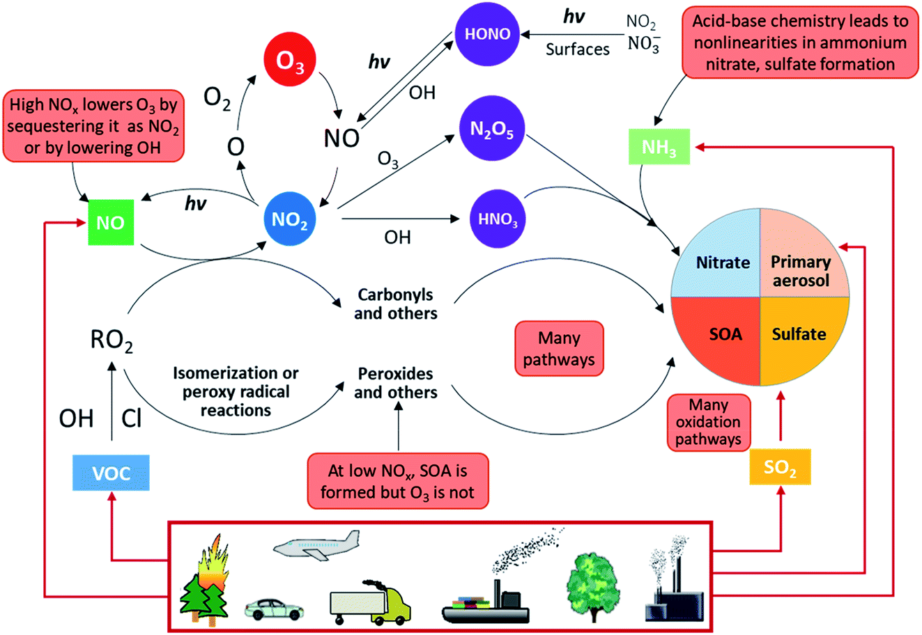 | ||
| Fig. 2 Overview of atmospheric physicochemical processes. The red boxes highlight the complexities, nonlinearities and uncertainties. Primary emissions are denoted by red arrows and secondary reactions are denoted by black arrows (adapted from Kroll et al.45). | ||
Gas phase chemistry
Gaseous pollutants (e.g., SO2, NOx, CO, CH4, CO2, VOCs, etc.) are emitted from both anthropogenic and natural sources. Anthropogenic sources are associated with human activities such as transportation, solvent consumption, and industrial emissions. Natural processes occurring in vegetation, soils, marine ecosystems, volcanos, biomass burning, animals, lightning, etc., also result in emissions of these pollutants. Biological sources are a subset of natural sources and include predominantly those of microbial activities in soils and vegetation. Emitted gaseous pollutants are subsequently oxidized by ambient free radicals including OH, O3, peroxy radicals (RO2), and NO3. OH is mainly produced by the UV-photolysis of O3 and is the most important radical because it reacts with most atmospheric species leading to oxidation reactions that produce O3 and secondary aerosols (SOA, sulfates, and nitrates) in the troposphere. The products and by-products of these oxidation reactions depend not only on the compound being oxidized, but also on the concentrations of other species that may affect this oxidation chemistry.46–50In urban environments, there are many VOC sources of anthropogenic and biogenic origin. VOC oxidation initiated by OH during the daytime produces a number of organic products of oxygenated functional groups, such as aldehyde, ketone, alcohol, carboxylic acid, hydroperoxide, percarboxylic acid, and peroxyacyl nitrate groups.51,52 The relative abundance of these products depends on the VOC structure, the NOx level, temperature, relative humidity (RH), and the solar intensity. Some compounds formed in the first oxidation step undergo additional oxidation reactions to yield multi-functional groups, and the resulting multi-generations of products are of lower volatility and higher solubility in comparison with their parent compounds.
NOx plays an important role in determining the fate of peroxy radical intermediates (HO2 and RO2). Under relatively clean (low-NO) conditions, peroxy radicals will react with other peroxy radicals or (in the case of RO2) will isomerize; under polluted urban conditions, peroxy radicals will react with NO, forming NO2, which rapidly photolyzes in the daytime, producing O3.53 However, the ambient levels of OH, HO2, and RO2 radicals not only depend on NOx but also simultaneously on the VOC abundance and VOC reactivity. This dual NOx and VOC–reactivity dependency ultimately controls the chemical regimes of O3 production. Therefore, successful emission control policies strongly depend on determining the chemical regimes of O3 production.
The sensitivity of O3 production to changes in concentrations of precursor VOCs and NOx is complex and nonlinear.53–55 Under high VOC concentrations and low NOx concentrations, O3 production rates increase with increasing NO concentrations (NOx limited) due to increases of NO2 through reactions of NO and peroxy radicals. But at higher NOx, O3 production rates decrease with increasing NOx (NOx saturated) due to OH and NOx termination reactions that form HNO3 and alkyl nitrates. The additional NOx also serves as a sink for OH radicals, slowing down the oxidation of VOCs and suppressing O3 production. NOx can also sequester O3 in temporary reservoirs such as NO2 and N2O5; in these conditions, lower NOx emissions can lead to higher O3 concentrations. This result could suggest that O3 production in polluted urban areas, as is the case in many megacities, may be in the NOx saturated regime.56–59 However, recent studies indicate that O3 production can have marked spatially different chemical regimes within megacities due to the heterogeneous distribution of VOC and NOx sources, VOC reactivity, and meteorological conditions.60,61
During the night-time, the oxidation of NO via O3 and organic radicals has two main effects: it depletes night-time O3 levels and accumulates NO2 and NO3 radicals that subsequently form N2O5 and HNO3 through heterogeneous reactions.62 This condition increases the early morning NO2/NO ratios and affects O3 production during the next day by increasing the contribution of excited oxygen atoms via NO2 photolysis. The accumulated NO2 and nitrate can also form HONO through surface-catalyzed reactions,63 further impacting the accumulation of free radicals.
Particulate matter
Particulate matter (PM) can be emitted directly from anthropogenic sources such as factories, power plants, automobiles, diesel engines, construction sites, unpaved roads, fires, etc. Natural sources of PM include sea salt, dust, pollen, volcanic eruptions, etc. Others form in complex reactions in the atmosphere of gaseous chemicals, such as VOCs, SO2 and NOx that are emitted from power plants, industries and automobiles, as described above. The most important PM is the “inhalable coarse particles” with diameters 10 μm and smaller (PM10), and “fine particles” with diameters 2.5 μm and smaller (PM2.5). PM10 are generated mainly by road traffic, agriculture, and mining, while PM2.5 are primary combustion particles or are formed as secondary pollutants. PM2.5 are more harmful to health because they can get deep into the lung. PM2.5 are also responsible for visibility impairment. PM2.5 and PM10 are regulated by USA clean air standards because of their known association with degraded visibility and detrimental health effects (US Clean Air Act, https://www.epa.gov/laws-regulations/summary-clean-air-act).64–66 While the widespread availability of PM2.5 measurements often make it the best proxy for epidemiological studies of populations, physiological studies of health effects have shown that the causes of cell degradation are most likely from specific toxic compounds, which are also regulated and include such compounds as polycyclic aromatic hydrocarbons (PAHs) that are associated with fossil fuel combustion and black carbon.The abundance and chemical constituents of PM2.5 vary considerably in urban cities, depending on the complex interplay between meteorology, emissions, and chemical processes.67,68Fig. 3 shows the average measured chemical composition of submicron PM (PM1), which typically comprises most of the PM2.5 for various megacities, urban areas, and outflow regions around the world.69 A substantial fraction of urban PM1 is organic aerosol (OA), which is composed of primary OA (POA, organic compounds emitted directly in the particle phase) and secondary OA (SOA, formed from chemical reactions of precursor organic gases). SOA is typically a factor of 2 to 3 higher than POA for these locations.
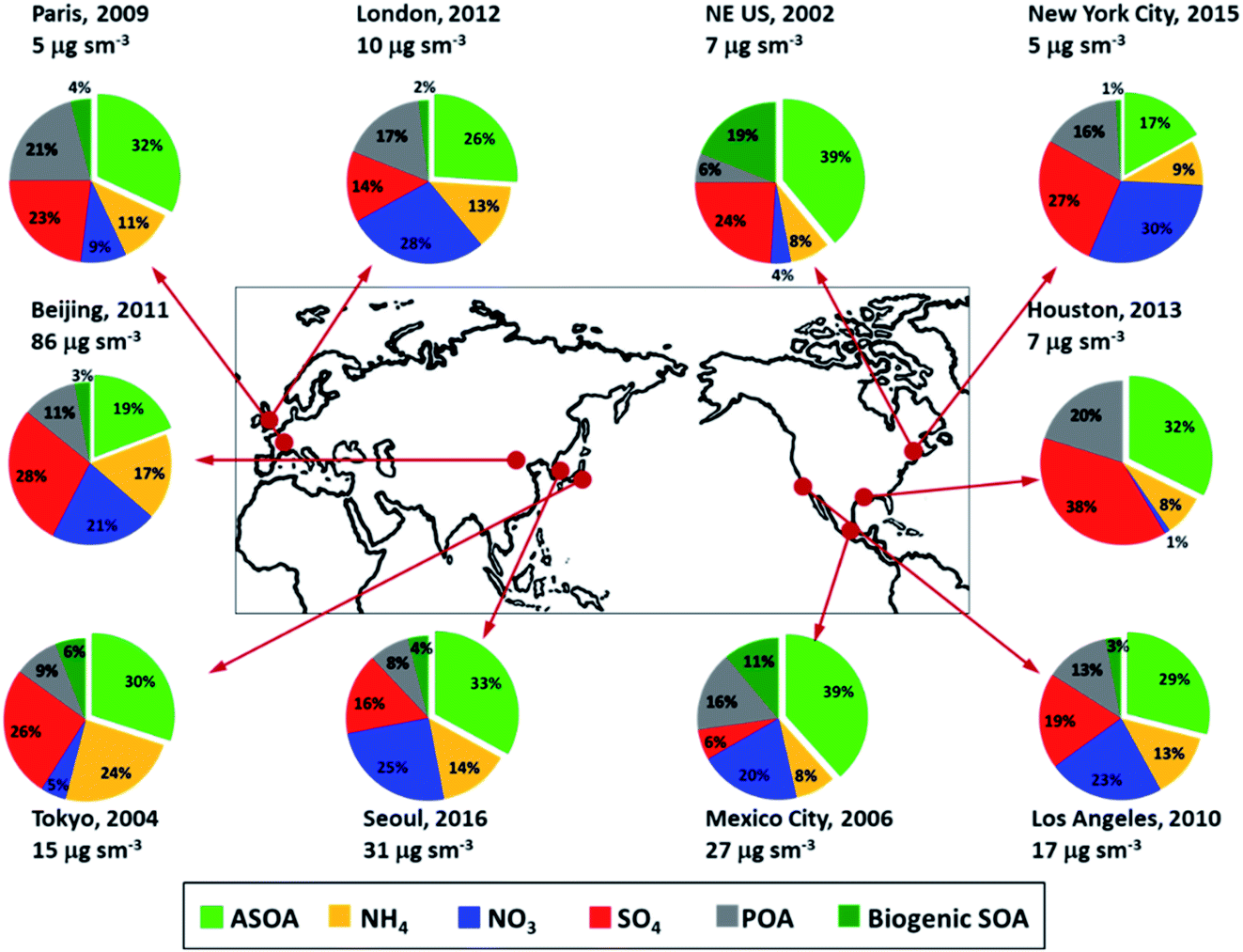 | ||
| Fig. 3 Non-refractory submicron composition measured in urban and urban outflow regions from field measurements, all in units of μg m−3 at standard temperature (273 K) and pressure (1013 hPa) (adapted from Nault et al.69). | ||
More recently, ultrafine particles (UFP, particles with diameter 0.1 μm or less) have become increasingly important in urban air because they are produced predominantly from local combustion processes with major contributions from vehicular exhaust and new particle formation (NPF) in cities.70–73 Particles that are smaller than 1 μm have both longer lifetimes and higher probability of penetration into alveolar sacs in the lungs, and even smaller “nanoparticles” (<100 nm in diameter) have been shown to have some of the most toxic exposures. Recent evidence suggests that nanoparticles and transition metals, which are also associated with fossil fuel combustion, may play an important role.74–79
Currently, particle mass concentration has been used for regulatory air quality standards. However, this metric accounts mainly for larger particles with larger mass, while particle number concentration (PNC) has been used as a metric for UFP, which are smaller with little mass. de Jesus et al.80 evaluated the hourly average PNC and PM2.5 from 10 cities over a 12 month period and observed a relatively weak relationship between the two metrics, suggesting that control measures aiming to reduce PM2.5 do not necessarily reduce PNC. It is important to monitor both PM2.5 and UFP for health impact assessment.
For developing effective pollution control strategies and exposure risk assessment, it is necessary to know the contribution of the various sources of pollutants. Several techniques have been used in source apportionment studies of PM, including chemical mass balance (CMB) and positive matrix factorization (PMF) analysis on filter-based chemical speciation data, carbon mass balance modeling of filter-based radiocarbon (14C) data, aerosol mass spectrometry or aerosol chemical speciation monitoring coupled with PMF. While significant progress has been made in evaluating the sources of pollutants, some sources remain poorly characterized, such as food cooking and open trash burning (see e.g., Molina et al.81 for Mexico City).
Pandis et al.82 investigated the PM pollution in five cities (Athens, Paris, Pittsburg, Los Angeles and Mexico City) and found that reductions of emissions from industrial and transportation related sources have led to significant improvements in air quality in all five cities; however, other sources such as cooking, residential and agricultural biomass burning contribute an increasing share of the PM concentrations. These changes highlight the importance of secondary PM and the role of atmospheric chemical processes, which complicate the source apportionment analysis. Xu et al. (DOI: 10.1039/D0FD00095G) evaluated the fine OC and PM2.5 in Beijing using different methods (CMB, PMF and AMS/ACSM-PMF) and found that the fine particles were mainly secondary inorganic aerosols, primary coal combustion and biomass burning emissions. Although there are some consistencies, modeled contributions for several sources differed significantly between the different methods, particularly for cooking aerosols.
New particle formation
New particle formation (NPF) has been observed under diverse environmental conditions and accounts globally for about 50% of the aerosol population in the troposphere.83 NPF occurs in two distinct stages.84 The first step involves the formation of a critical nucleus during the transformation from vapor to liquid or solid. The second step is the growth of the critical nucleus to a larger size (>1–3 nm) that competes with the removal of newly nucleated nanoparticles by preexisting aerosols. Various species have been suggested to account for aerosol nucleation and growth, including sulfuric acid, organic acids from oxidation of VOCs, ammonia/amines, and ions.85–91 However, there is a lack of consistent mechanisms to explain NPF under diverse atmospheric conditions, especially in heavily polluted atmosphere of megacities.92–94Extensive efforts have been made to elucidate the fundamental mechanism relevant to atmospheric NPF from field measurements, laboratory experiments, and theoretical calculations. Previous field studies include measurements of ultrafine particles down to approximately 1 nm in size, gaseous concentrations of nucleating precursors (such as H2SO4, NH3, and amines), and pre-nucleation clusters.95,96 Numerous laboratory experiments have been conducted to understand aerosol nucleation.92,97–99 In addition, theoretical investigations of aerosol nucleation have been carried out to determine the stability and dynamics of pre-nucleation clusters using thermodynamic data from quantum chemical calculations.100–102
NPF events occur with a frequency of 50, 20, 35, and 45% in spring, summer, fall, and winter, respectively, in Beijing.102–104 NPF events have been occasionally measured in Houston during several campaigns.105,106 In addition to the correlation with elevated SO2,107 the contribution of secondary condensable organics to NPF is implicated in Houston.108 On the other hand, NPF events are rarely measured in Los Angeles.109 One plausible explanation is that the heavy accumulation of pre-existing particles and low levels of SO2 lead to unfavorable conditions for aerosol nucleation in the Los Angeles basin.110 NPF events are frequently observed during field campaigns in Mexico City81,111,112 and are usually accompanied with a high level of SO2,113 indicating that the oxidation of SO2 contributes to the formation and growth of freshly nucleated particles. The polluted layer substantially ventilated from the Mexico City basin represents another potential factor in driving NPF in the afternoon, which is characterized by a decrease in pre-existing particle concentrations preceding the NPF events.114
A recent study shows the striking formation of NPF in urban air by combining ambient and chamber measurements.91 By replicating the ambient conditions (i.e., temperature, relative humidity, sunlight, and the types and abundance of chemical species), the existing particles, photochemistry, and synergy of multi-pollutants play a key role in NPF. In particular, NPF is dependent on preexisting particles and photochemistry, both of which impact the formation and growth rates of freshly nucleated nanoparticles. Synergetic photooxidation of vehicular exhaust provides abundant precursors, and organics, rather than sulfuric acid or base species, dominating NPF in the urban environment.
Another laboratory chamber study by Wang et al.115 reported that airborne particles can grow rapidly through the condensation of ammonium nitrate (NH4NO3) under conditions typical of many urban environments in wintertime, such as Beijing and Delhi. NH4NO3 exists in a temperature-dependent equilibrium with gaseous NH3 and HNO3, but NH4NO3 can quickly condense onto newly formed clusters at temperatures below 5 °C, allowing the clusters to reach stable particle sizes before they are scavenged by other existing particles in the atmosphere. Moreover, at temperatures below −15 °C, NH3 and HNO3 can nucleate directly to form NH4NO3 particles. The formation of new particles through NH4NO3 condensation could become increasingly important as the SO2 emissions continue to reduce due to pollution controls implemented in many cities. This may in turn imply the importance of controlling NOx and NH3 emissions.
Based on the observations in Beijing over a period 14 months, Kulmala et al. (DOI: 10.1039/D0FD00078G) found that almost all present-day haze episodes in Beijing originate from NPF, suggesting that air quality can be improved by reducing the gas phase precursors for NPF, such as dimethyl amine, NH3 and further reductions of SO2 emissions, as well as anthropogenic organic and inorganic gas-phase precursor emissions.
Secondary organic aerosol
Formation of secondary organic aerosol (SOA) involves a complex multiphase process and represents one of the most poorly understood topics and a frontier research area in atmospheric chemistry.67,116–118 This complex process consists of photochemical oxidation, nocturnal reactions, heterogeneous reactions, nucleation and condensation/partitioning.68,119 A conventional view is that SOA formation is dominated by absorptive partitioning of low- and semi-volatile oxidation products associated with VOCs oxidation by OH, NO3 and O3. VOCs species are characterized by functionality, reactivity and aerosol formation potential, which are different from single precursors of secondary inorganic aerosols. SOA can be formed by some primary organic aerosol (POA) species, which evaporate and are oxidized, further repartition into aerosols.120,121 Evidence from laboratory, field, and theoretical calculations have also suggested that aqueous phase chemistry represents a significant pathway for SOA production.35,122–128Atmospheric models typically underestimate the SOA mass measured in field studies if only traditional SOA precursors are considered.122,129–131 Inclusion of non-traditional SOA precursors, such as organic gases from POA evaporation and di-carbonyls, has helped to bring better closure between models and observations.132–136 However, there are still inconsistencies between modeled and measured SOA yields, which can be explained by several factors, including incorrect emission inventories, missing precursors, and unaccounted processes of gas-to-particle conversion.13,68
Nault et al.69 investigated the production of anthropogenic SOA (ASOA) in urban areas across three continents (see Fig. 3) and observed that it is strongly correlated with the reactivity of specific VOCs; the differences in the emissions of aromatics and intermediate- and semi-volatile organic compounds (IVOC and SVOC) influence the ASOA production across different cities. Emissions from fossil fuel sources (e.g., gasoline, diesel, kerosene, etc.) and volatile chemical products (VCPs, such as personal care products, cleaning agents, coatings, etc.) contribute nearly similar amounts to estimated ASOA, further supporting the important role of VCPs in urban air quality.13
Sulfate formation
The main source of the sulfate in the atmosphere is the multiphase oxidation of SO2, including gas-phase oxidations by OH and stabilized Criegee Intermediates (sCI), aqueous reactions in cloud or fog droplets, and heterogeneous reactions associated with aerosol water.137 The gas-phase oxidation of SO2 is dominated by the reaction with OH radicals. At the typical atmospheric level of OH radical, the lifetime of SO2 from the reaction with OH is about one week.67 Additionally, the sCI chemistry has been proposed to potentially contribute substantially to the SO2 oxidation, and exert profound effects on sulfate formation.138The aqueous-phase conversion of dissolved SO2 to sulfate driven by O3 and hydrogen peroxide (H2O2) is an important chemical formation pathway in cloud/fog water, but the two SO2 oxidation pathways still cannot close the gap between field observations and modeling studies.139 Aqueous SO2 oxidation by O2 catalyzed by transition metal ions (TMI) in models has improved sulfate simulations,140 and recent studies have further revealed the enhanced effect of TMI during in-cloud oxidation of SO2 (ref. 141). However, during wintertime haze days free of cloud or fog in North China, rapid sulfate production has been observed142,143 showing that the sulfate formation mechanism is still not well understood.
A laboratory/field study of wintertime haze events in Beijing and Xi’an has indicated that the aqueous oxidation of SO2 by NO2 is key to efficient sulfate formation under the conditions of high RH and NH3 neutralization,143,144 Li et al.145 proposed a SO2 heterogeneous formation pathway, in which the SO2 oxidation in aerosol water by O2 catalyzed by Fe3+, is limited by mass resistance in the gas-phase and gas–particle interface, and closes the gap between model and observation. A recent experimental study has highlighted that the oxidation of SO2 by H2O2 in hygroscopic, pH-buffered aerosol particles occurs more efficiently than under cloud water conditions, because of high solute strength.146 Furthermore, another recent study147 has unraveled a novel sulfate formation mechanism, showing that SO2 oxidation is efficiently catalyzed by black carbon (BC) in the presence of NO2 and NH3, even at low SO2 levels (down to a few ppb) and an intermediate RH range (30–70%). The sulfate formation mechanism during wintertime haze days in China is still controversial considering the uncertainties of the aerosol pH value, rather low oxidants level, and possible loss of active sites in BC.
Nitrate formation
The gas-phase reaction between NO2 and OH to form nitric acid is the dominant formation pathway for nitric acid during the daytime,148 corresponding to a lifetime of about a day for NO2. The heterogeneous reaction between HNO3 and NH3 in the particle-phase to form ammonium nitrate also regulates the gaseous HNO3 concentration. Depending on the RH, the ammonium nitrate formed exists in a solid or an aqueous form consisting of NH4+ and NO3−, and the correlation between gaseous HNO3 and particle-phase nitrate is dependent on equilibrium partitioning.149 Also, amines react with nitric acid and ammonium nitrate to form aminium nitrates by acid–base and replacement reactions, respectively.90 The heterogeneous hydrolysis reaction of dinitrogen pentoxide (N2O5) on surfaces of deliquescence aerosols dominates the nocturnal nitrate formation in the urban atmosphere.150,151 There is also substantial evidence of nitrate enhancement in fog conditions.35 In addition, although N2O5 is photolytically liable during daytime, the heterogeneous N2O5 hydrolysis still contributed 10% of HNO3 during heavy haze days in winter, which is caused by substantial attenuation of incident solar radiation by clouds and high PM2.5 mass loading.152 In addition to inorganic nitrate, the oxidation reactions of VOCs in the presence of NO2 produce peroxy nitrates (RO2NO2) and strongly-bounded mono and multifunctional alkyl nitrates (RONO2). There are two main pathways for RONO2 production: OH-initiated oxidation of hydrocarbons in the presence of NOx during the daytime, and nitrate radical (NO3)-initiated oxidation of alkenes during the nighttime.153Aerosol radiative effect
Aerosol radiative forcing has been identified as one of the largest uncertainties in climate change research.154 Aerosols influence Earth’s radiative balance directly by scattering or absorbing solar radiation to cool or warm the atmosphere and dim the surface (direct effects); further induce adjustments of the surface energy budget, thermodynamic profile and cloudiness (semi-direct effects); and indirectly by serving as cloud condensation nuclei (CCN) and ice nuclei (IN) to change cloud properties such as cloud lifetime, reflectivity and composition (indirect effects). IPCC (2013) has used the new terminology of aerosol–radiation interaction (ARI) to refer to the combination of aerosol direct and semi-direct effects, and aerosol–cloud interaction (ACI) to refer to the aerosol indirect effects. The amount of forcing depends on their physical (size and shape) and chemical (surface chemistry, hygroscopicity, etc.) properties and on their residence times in the troposphere.Aerosol radiation interaction has also significantly contributed to the PM pollution during haze days.68 It is well established that ARI cools the surface but heats the air aloft, increases the atmospheric stability, enhances accumulation and formation of PM2.5 in the planetary boundary layer (PBL), and eventually deteriorates the air quality during haze days.155–157 Wu et al.157 have revealed that the ARI contribution to near-surface PM2.5 concentrations increased from 12% to 20% when PM2.5 concentrations increased from 250 to 500 μg m−3 during a persistent and severe PM pollution episode in the North China Plain. However, modification of photolysis caused by aerosol absorbing and/or scattering solar radiation (referred to as aerosol–photolysis interaction or API) changes the atmospheric oxidizing capability and influences secondary aerosol formation. Coatings also affect the ratio of absorption to scattering, and these control changes in radiative forcing.158 Simulations have revealed that API hinders secondary aerosol formation and substantially mitigates the PM pollution caused by ARI.159
It is worth noting that ARI or API is highly sensitive to the single scattering albedo (SSA) that is dependent on aerosol composition, particularly regarding absorbing aerosols including BC and brown carbon (BrC).159 Primary BC and BrC aerosols undergo chemical transformation in the atmosphere, by coating with organic and inorganic constituents, commonly referred to as the aging process.158 Aging of primary aerosols not only changes the particle mixing state (i.e., from externally to internally), but also alters the particle properties, including the morphology, hygroscopicity, and optical properties, further enhancing aerosol absorption capability.117,160–162
Air quality management in megacities
Air quality management in megacities is a dynamic process. The design of effective emission control strategies in megacities requires detailed information on the pollutant concentrations and meteorological parameters provided by air quality monitoring networks and the key sources of pollution and their spatial distribution, characterized by emission inventory. In addition, scientific research is needed to provide information on the transport and transformation of pollutants in the atmosphere. Combining air quality observations, emission inventory, meteorology, and atmospheric chemistry enables air quality models to be developed which can be used to evaluate past episodes, assess different emission reduction strategies, and make air quality forecasts. Changes in emissions and other circumstances may identify new air quality problems and require updating and enforcing policy measures.Since 1987, the WHO has produced air quality guidelines designed to inform policy makers and to provide appropriate targets in reducing the impacts of air pollution on public health. Currently, many countries have established ambient air quality standards to protect the public from exposure to harmful level of air pollutants and are an important component of national risk management and environmental policies. National standards vary according to the approach adopted for balancing health risks, technological feasibility, economic, political and social considerations, as well as national capability in air quality management. Some countries set additional standards for lead and CO. Table 1 presents the current air quality standards for O3, PM10, PM2.5, SO2, CO, Pb and NO2 for China, India, Mexico and the USA, together with the WHO guidelines.163
| Mexicoa | China | India | United Statesa | WHO | |
|---|---|---|---|---|---|
| a Air quality standards for O3, SO2, NO2, and CO in Mexico and the USA are reported in parts per million (ppm); they are converted to μg m−3 for comparison at a reference temperature of 298 K and barometric pressure of 1 atm. b The annual fourth-highest daily maximum 8 hour concentration, averaged over 3 years. c Lead: in areas designated nonattainment for the Pb standards prior to the promulgation of the current (2008) standards, and for which implementation plans to attain or maintain the current (2008) standards have not been submitted and approved, the previous standards (1.5 μg m−3 as a calendar quarter average) also remain in effect. | |||||
| Pollutant | Max. limit | Avg. ann. max. | Max. limit | Max. limit | Guidelines |
| (μg m−3) | (μg m−3) | (μg m−3) | (μg m−3) | (μg m−3) | |
| O3 | 186 (1 h mean) | 200 (1 h) | 180 (1 h) | 100 (8 h) | |
| 137 (8 h mean) | 160 (8 h) | 100 (8 h) | 137 (8 h)b | ||
| PM10 | 75 (24 h mean) | 150 (24 h) | 100 (24 h) | 150 (24 h) | 50 (24 h) |
| 40 (ann mean) | 70 (ann) | 60 (ann) | 50 (ann) | 20 (ann) | |
| PM2.5 | 45 (24 h mean) | 75 (24 h) | 60 (24 h) | 35 (24 h) | 25 (24 h) |
| 12 (ann mean) | 35 (ann) | 40 (ann) | 12 (ann, primary); 15 (ann, secondary) | 10 (ann) | |
| SO2 | 290 (24 h mean) | 500 (1 h) | 80 (24 h) | 1950 (1 h) | 20 (24 h) |
| 520 (8 h mean) | 150 (24 h) | 50 (ann) | 1300 (3 h) | 500 (10 min) | |
| 65 (ann mean) | 60 (ann) | ||||
| CO | 10 (1 h) mg m−3 | 4 mg m−3 (1 h) | 40 mg m−3 (1 h) | ||
| 12.5 mg m−3 (8 h mean) | 4 (24 h) mg m−3 | 2 mg m−3 (8 h) | 10 mg m−3 (8 h) | ||
| Pb | 1.5 (3 month mean) | 1 (ann) | 1 (24 h) | 0.15 (3 month)c | |
| 0.5 (3 month) | 0.5 (3 month) | ||||
| NO2 | 400 (1 h mean) | 200 (1 h) | 80 (24 h) | 200 (1 h) | |
| 80 (24 h) | 40 (ann) | 100 (ann mean) | 40 (ann) | ||
| 40 (ann) | |||||
The WHO estimated that about 90% of the world’s population breathe polluted air, many of the world’s megacities exceed WHO’s guideline levels for air quality by more than 5 times.164Fig. 4 shows the annual average of PM2.5 for a three-year period (2017, 2018, and 2019) for the megacities where data is available; this includes London, Seoul and Chengdu.
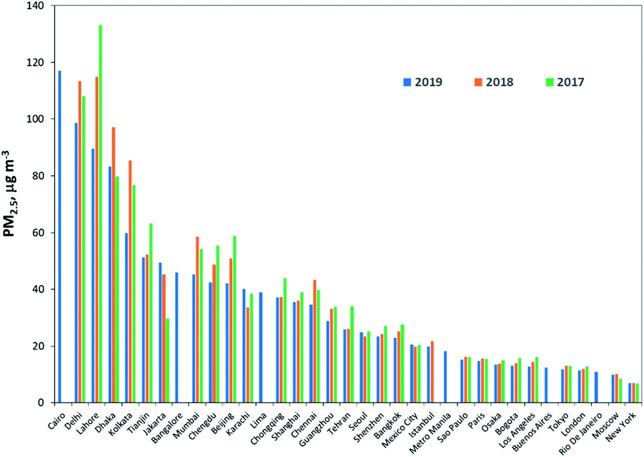 | ||
| Fig. 4 Annual average of PM2.5 for the three-year period 2017–2019. Source: IQAir.165 Data sources include real-time, hourly data from government monitoring stations, validated PM2.5 monitors operated by private individuals and organizations. Cairo, Rio de Janeiro, Bangalore, and Lima are from WHO166 data (for the year 2015 or 2016). | ||
The data were compiled by IQAir165 from real-time, hourly data from government monitoring stations, validated PM2.5 monitors operated by private individuals and organizations. Ideally, the monitoring data used to calculate the average annual PM concentrations should be collected throughout the year, for several years, to reduce bias owing to seasonal fluctuations or to a non-representative year. However, data for most cities are not available for trend analysis. Some of the megacities were not included in the report; the data were taken from WHO166 for a single year reported in 2015 or 2016.
The PM2.5 levels for all the megacities shown in Fig. 4, with the exception of New York, are above the WHO guideline value of 10 μg m−3. The megacities with the highest PM2.5 concentrations are located in South Asia; however, comparison of the three-year data show reduction in the PM2.5 levels in the cities from 2018 to 2019. Much of this can be attributed to increased monitoring data, economic slowdown, favorable meteorological conditions and government actions. For example, 2019 marked the launch of India’s first National Clean Air Program, which set PM2.5 and PM10 targets and outlined new strategies for tackling air pollution. However, India still has a relatively limited air quality monitoring network, with many communities lacking access to real-time information.167
The data shown in Fig. 4 are the annual average; however, there is a large seasonal variation for some cities (Delhi, Lahore, Dhaka, Kolkata), as shown in Fig. 5, due to geographical location and prevailing meteorology. The PM2.5 concentrations are the highest in November to January, and the lowest from July to September, as monsoon rains wash out airborne particulates, leading to cleaner air. During the winter, emissions from residential heating, burning of crop residues, and intensive brick production lead to higher PM2.5 concentrations in these cities. The landlocked geography of Delhi and the coastal location of Mumbai influence the distribution of air pollutants in the two cities.168
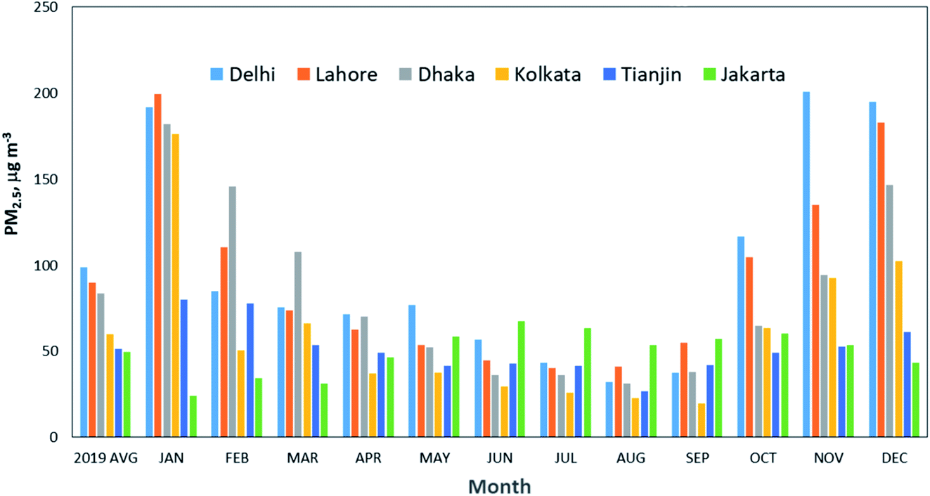 | ||
| Fig. 5 Monthly average of PM2.5 concentrations for the six megacities with the highest PM2.5 concentrations in 2019. Source: IQAir.165 | ||
Lahore ranks as one of the megacities with the highest annual PM2.5 concentrations, weighted by city population. Until recently, there was no government monitoring in Pakistan. The data provided in the IQAir165 report (2019) comes from low-cost sensors operated by individuals and non-governmental organizations. Recently the Pakistan government cited air pollution as a key priority and has reinstated the monitoring infrastructure in Lahore. Current anti-smog measures include stricter emission standards on factories and penalties for high-polluting vehicles and farmers burning crop stubble.
Although more countries are taking action and more cities are now included in the air quality database, there are still many cities that do not have ambient monitoring and their residents do not have access to air quality information where pollution levels may be high. For example, South America is the most urbanized region of the world; five of the megacities are located in this continent: Bogotá (Colombia), Buenos Aires (Argentina), Rio de Janeiro (Brazil), São Paulo (Brazil) and the metropolitan area of Lima-Callao (Peru). Recently, Gómez Peláez et al.169 reviewed the air quality trends of the criteria pollutants collected by the automatic monitoring networks of 11 metropolitan areas in South America, including four megacities (Rio de Janeiro, São Paulo, Buenos Aires, and Lima). Despite concerted efforts to monitor air quality, the data provided by environmental authorities in some cities are of poor quality, making it difficult to assess the air quality trends and take action for critical air pollution episodes. Integration of the emission from the whole continent and their application in an air quality model are essential to investigate the effect of long-range transport and to construct air quality and emission control strategies for the entire region. Integrated coordination due to transboundary pollution transport, mainly from the biomass burning in the Amazon basin, is essential, especially considering the record-breaking number of Amazon fires in 2019 and again in 2020. Analysis of an aerosol particles’ chemical composition and optical properties during the biomass burning season in 2014 showed that, depending on the wind direction, smoke plumes from central Brazil and southern regions of the Amazon basin can be transported over São Paulo.170
In February 2020, the United Nations Environment Programme (UNEP), together with the UN-Habitat and IQAir, launched the world’s largest air quality platform, bringing together real-time air pollution data from over 4000 contributors, including governments, citizens, communities, and private sectors.171 This partnership covers more than 7000 cities worldwide and aims to empower governments to take action to improve air quality, allowing citizens to make informed health choices, and businesses to make investment decisions promoting a cleaner and greener environment.
The following describe the air quality trends and air quality management programs for Los Angeles, the Mexico City metropolitan area and four Chinese megacities. While the differences in the governance, economics, and culture of the megacities greatly influence the decision-making process, all have overcome severe air pollution and have made significant progress in reducing concentrations of harmful pollutants by implementing comprehensive integrated air quality management programs. The experience can be valuable for other megacities.
Air quality in the Los Angeles basin
The Los Angeles metropolitan area had 12.5 million inhabitants in 2018 (UN, 2018a) and is the second-most populated urban area in the United States, after the New York–Newark metropolitan area. The multi-county South Coast Air Basin (SoCAB), which consists of Orange County and the urban portion of Los Angeles, Riverside, and San Bernardino Counties with a population of 18 million, is one of the air basins in California designated for air quality management (http://www.aqmd.gov). The basin is bordered by the Pacific Ocean on the west and mountains on the other three sides, which limit horizontal ventilation. During the summer, the coastal air basin is often under the influence of a large-scale subsidence inversion that traps a layer of cool marine air. Pollutants emitted from various sources during the day are pushed by onshore sea breeze to the inland valleys, undergoing photochemical reactions and producing O3 and other oxidants. Stagnant high pressure systems with subsidence aloft allow pollutants to accumulate near the ground, causing high smog episodes.Following the recognition of Los Angeles photochemical smog as a severe environmental problem in the 1940s, comprehensive emissions control efforts have been implemented by the air quality management authorities, the California Air Resources Board (CARB) and the South Coast Air Quality Management District (SCAQMD) principally, particularly in the transportation sector, which plays a major role in the air pollution problem. The urban center is decentralized; major commercial, financial and cultural institutions are geographically dispersed, relying on a vast network of interconnected freeways. The emissions control measures included the introduction of unleaded gasoline and an eventual complete ban of lead in gasoline, three-way catalytic converters, stringent NOx control for ozone and PM2.5, low-sulfur fuels, and diesel particle filters. Other regulations such as controls on power plants and boilers have reduced smog-forming oxides of nitrogen emissions, rules on consumer products such as paints and solvents have limited volatile organic compounds, and other controls on gasoline components, chrome platers, dry cleaners, and other sources have reduced levels of airborne toxics.6,172
Other emission sources include goods movement sources, such as railroads, ocean-going vessels, commercial harbor craft, cargo handling equipment, drayage trucks, and transport refrigeration units. California adopted the first-in-the-nation regulation requiring ocean-going vessels to use cleaner fuel when near the California coast in 2008, which has been effective in reducing SO2 emission from ships.173 Emissions from ports have also been reduced by making shore power available to docked ships that previously idled their engines, while the more polluting drayage trucks are either removed from service or retrofitted.6 The Advanced Clean Car Regulation (https://ww2.arb.ca.gov/our-work/programs/advanced-clean-cars-program) is the latest of a series of technology-forcing standards aimed at limiting passenger vehicle emissions and reducing smog as well as mitigating climate change.174 As a result of the stringent emissions reduction measures, peak ozone levels and PM2.5 concentrations in Los Angeles today are about one third of their level in 1970. Nevertheless, the ozone concentration is frequently still above the current USA ambient 8 h ozone standard of 70 ppb (see Fig. 6).
 | ||
| Fig. 6 Comparison of air quality trends (for O3 and PM) in the Mexico City metropolitan area (MCMA) and South Coast Air Basin (SoCAB) using the same metrics. Graphs plotted with data from SIMAT (http://www.aire.cdmx.gob.mx/) and SoCAB (http://www.aqmd.gov). | ||
One of the main challenges is that a substantial fraction of the ozone in Southern California is transported into the region from outside its border, which is not subject to local control. This includes the baseline ozone concentrations, which are not affected by continental influences, such as ozone transported from the Pacific175 and the background ozone (the ozone concentration that would be present if anthropogenic precursor emissions were reduced to zero), which are affected by continental influences such as deposition to continental surfaces, vegetation, production from natural ozone precursors (e.g. from trees, soils and lightning).176 This could be as high as 89% of the USA NAAQS (62.0 ± 1.9 ppb) and that about 35 years of additional emission control efforts will be needed to meet the NAAQS.
Altuwayjiri et al. (DOI: 10.1039/D0FD00074D) investigated the long-term variations in the contribution of emission sources to ambient PM2.5 organic carbon (OC) in the Los Angeles basin and the effect of the regulations targeted tailpipe emissions during 2005–2015. They found a significant reduction in the absolute and relative contribution of tailpipe emissions to the ambient OC level, while the relative contribution of non-tailpipe emissions (road dust resuspension, tire dust, and brake wear particles) increases over the same period, suggesting that the regulations were effective but also underscore the importance of regulating non-tailpipe emissions.
Recent wildfires in California have markedly increased, worsening air quality in much of the region. A warmer and drier climate is expected to lead to more frequent and more intense fires near or within the populated areas, threatening to undo the significant improvement in air quality after decades of implementing the Clean Air Act.27–29 Long-term monitoring and reevaluation of forest management strategies will be needed to address the wildfire problem as climate change continues to bring hotter and drier conditions conducive to wildfire activity.177
Air quality in the Mexico City metropolitan area
Comparing California’s air quality with that of other cities (and countries) shows how cities around the world have benefited by adopting strategies and control technologies pioneered in Los Angeles. An example is the Mexico City metropolitan area (MCMA).178 In late 1980s to early 1990s, all criteria pollutants frequently exceeded the AQ standards, with ozone peaking above 300 ppb 40–50 days a year, leading Mexico City to be ranked as the most polluted megacity in the world at that time.179 Since the 1990s, the Mexican government has made significant progress in improving the air quality of the MCMA by developing and implementing successive comprehensive air quality management programs that combined regulatory actions with technological change based on scientific, technical, social, and political considerations. Vehicle emissions reduction focused on adapting advanced technology and improved fuel quality that had been successfully implemented in other countries, especially in California, including removal of lead from gasoline, mandatory use of catalytic converters, reduction of sulfur content in diesel fuel, reinforcement of vehicle inspection and maintenance, and mandatory “no driving day” rule. Emissions reduction measures for industry and commercial establishments included closing of an oil refinery, relocating high polluting industries outside the valley, substituting fuel oil in industry and power plants with natural gas, and reformulating liquefied petroleum gas (LPG) for cooking and water heating. As the result of implementing comprehensive air quality improvement programs, the city has significantly reduced the concentrations of all criteria pollutants,180 as shown in Fig. 6, top left panel. The figure also shows a comparison of the air quality trends (for O3 and PM) in the MCMA with the SoCAB using the same metrics. Both air basins show similar trends, O3 and PM10 have decreased significantly in both air basins, but even more rapidly in the MCMA, so that the concentrations in the MCMA have approached those in SoCAB in recent years despite a large difference in the financial and human resources and institutional capacity, which are essential for developing and implementing emission control programs.Field measurements studies conducted in the MCMA during MCMA-2003 (ref. 112) and MILAGRO-2006 (ref. 81) showed that ozone formation was generally VOC-limited within the urban core, while mostly NOx-limited in the surrounding area depending on the prevailing meteorology,56–58 and that O3 production might continue in the outflow for several days due to the formation of peroxyacetyl nitrate (PAN), which could regenerate NOx and contribute to regional O3 formation.181 A recent study by Zavala et al.60 shows that there is an overall reduction in the VOC–OH reactivity during the morning hours in the urban area with large spatial variability, implying a large spatial variability in O3 production, which in turns suggests spatially different O3 sensitivity regimes to precursor gases. While alkanes (from leakage and unburned LPG used for cooking and water heating) are still key contributors to VOC–OH reactivity, the contribution from aromatic and alkene species has decreased, consistent with reduction of VOCs from mobile sources. Changes in ozone production suggest that increases in the relative contributions from highly oxygenated volatile chemical products, such as consumer and personal care and solvent use, are responsible for sustained high O3 levels in recent years. The study also found a significant increase in NO2/NO ratios, suggesting changes in the night-time accumulation of radicals that could impact the morning photochemistry. The results suggest a need for a new field study of radical budgets in the MCMA, expanding measurements of VOCs to include oxygenated species, and using the data to support modeling studies in the design of new air quality improvement programs.
The MCMA faces additional challenges from regional contributions. Urban expansion of the MCMA has produced the megalopolis, consisting of Mexico City and contiguous municipalities of six surrounding states. The Megalopolis Environmental Commission (CAMe, https://www.gob.mx/comisionambiental) was created in 2013 to coordinate the regional policies and programs; however, the different administrative and legislative jurisdictions and the available resources have created an ongoing challenge. With the exception of the MCMA, there is limited air quality monitoring and air pollution studies in the other states, making it difficult to evaluate the regional air quality and the impacts of pollutants in the region.9
Burning of regional biomass is a major contributor of fine particles to the MCMA during air pollution episodes (http://www.aire.cdmx.gob.mx). During the dry season, agricultural and forest fires in the surrounding areas are frequent, the wind transports air masses enriched with organic aerosols, VOCs, as well as other reactive gases to the MCMA, severely impacting the air quality.20 Lei et al.182 evaluated the impact of biomass burning in the MCMA and found that biomass burning contributed significantly to primary organic aerosol (POA), secondary organic aerosol (SOA), and elemental carbon (EC) locally and regionally but has relatively little effect on O3. Despite the important contribution of biomass burning to local and regional air quality, the authorities did not include fire mitigation in the air quality management strategies. In May 2019, following a severe air pollution episode caused by regional wildfires, the authorities announced new action contingencies, adding PM2.5 threshold level, in addition to O3 and PM10, to the contingency plan.
Air quality in Chinese megacities
Of the 33 megacities in the world in 2018, six are located in the People’s Republic of China (Chongqing, Shanghai, Beijing, Tianjin, Guangzhou, and Shenzhen) according to a UN report,3 although according to the China Statistics Bureau, there are 15 cities with more than 10 million inhabitants due to different city boundaries defined in the two datasets.167 Many of these megacities are suffering from severe air pollution caused by rapid socio-economic development, motorization and industrialization, following the “reform and open-up policy” beginning in the late 1970s, which transformed China into the second-largest economy in the world, after the USA.As a global hub for manufacturing, the heavy industries, including production of iron and steel, other nonmetal materials and chemical products, play an important role in the Chinese economy, resulting in huge consumption of energy and large emissions of air pollutants. In addition, more and more people are moving from rural to urban areas, leading to a fast expansion of cities and an increasing demand for vehicles, contributing to severe air pollution.
Faced with increasing pressure on the environment in urban development, the Chinese government launched the Action Plan for Air Pollution Prevention and Control (Action Plan) in September 2013 (http://www.gov.cn/zwgk/2013-09/12/content_2486773.htm), which stated the development targets and roadmap for 2013–2017. The Action Plan provides the framework for air pollution control measures in cities, covering capacity building, emission reduction measures and supporting measures. The implementation of a series of control measures, including coal combustion pollution control, vehicle emission control and VOCs control, have resulted in the reduction of most pollutants and a large decrease in PM2.5 concentrations.167 However, according to a government report,183 74.3% of 74 key cities exceeded the NAAQS of annual mean PM2.5 concentrations (35 μg m−3) in 2017.
As shown in Fig. 7, while the concentration of most pollutants have decreased for each city, O3 was not effectively controlled (red line). Also, the annual mean PM2.5 concentrations still exceeded the NAAQS of China, except Shenzhen, the first city that met the PM2.5 standard. The exceeding of the PM daily average concentration often occurred during the cold winter from November to February, while the maximum daily 8 h average concentration of O3 is more likely to exceed in the summer during the afternoon, according to the local monitoring data (China National Environmental Monitoring Center, http://www.cnemc.cn/en/).
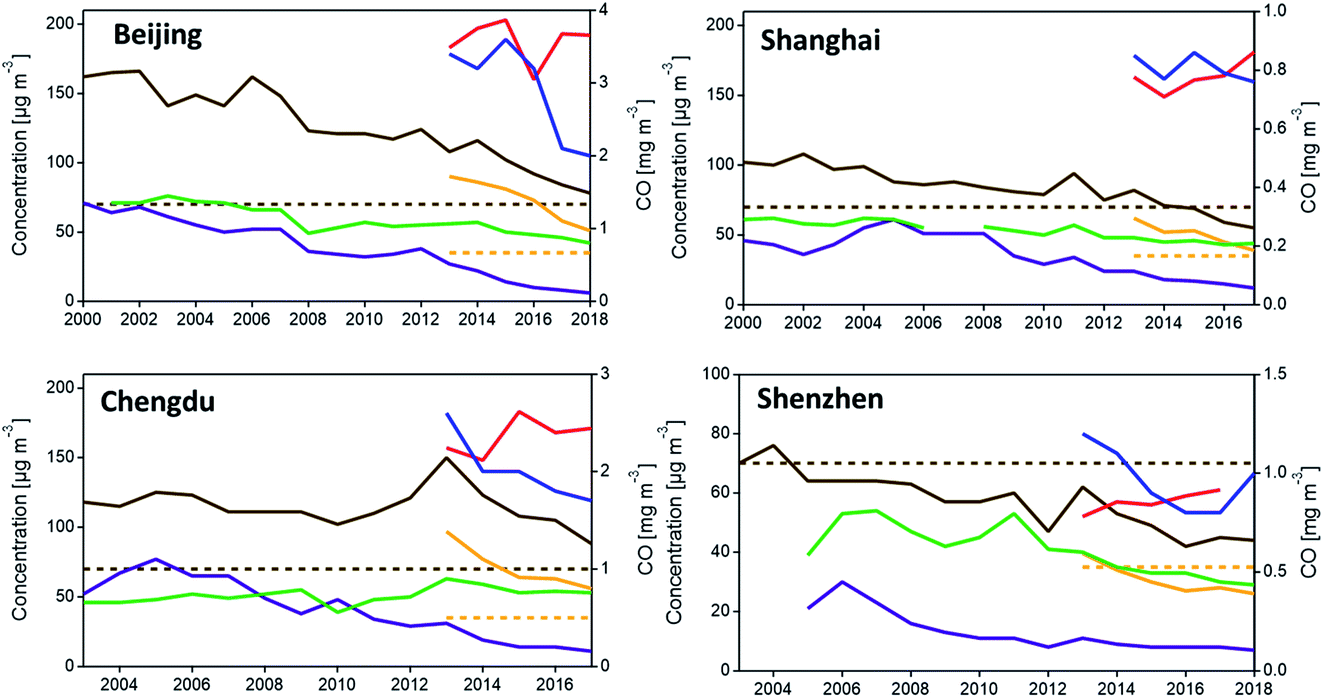 | ||
| Fig. 7 Air quality trends (annual average) for Beijing, Shanghai, Shenzhen and Chengdu. Red, O3; blue, CO; green, NO2; purple, SO2; brown, PM10 (dotted brown line, PM10 standard); yellow, PM2.5 (dotted yellow line – PM2.5 standard). Note O3 level = annual average of daily 8 h mean concentration. Sources: China Statistics Bureau and Beijing Environmental Protection Bureau; China Statistics Bureau and Shanghai Environmental Protection Bureau; China Statistics Bureau and Shenzhen Environmental Protection Bureau; China Statistics Bureau and Chengdu Environmental Protection Bureau (data compiled by W. Wan167). | ||
Although the major sources of emissions differ among the four cities, in general, vehicle emissions remain the primary source of air pollution and contribute significantly to VOC, NOx, CO, and PM2.5 (including BC). The primary source of SO2 is fossil fuel combustion from industry and mobile vehicles; while road and construction dust is the main source of PM10, and agriculture is the primary source of NH3.
Vehicle emission control has been a priority of air quality management, and the cities have continuously tightened emission standards for new gasoline and diesel vehicles; promoting the use of electric vehicles through subsidies.167 Shenzhen is the first megacity in China and in the world to adopt electric vehicles for the entire public transportation system. However, as a coastal city, diesel trucks carrying large amounts of cargo is the primary source of local emissions and ocean-going vessels, contributing a large portion of SO2 due to the use of low-quality heavy fuel oil. Emission control policies for the port area and the ocean-going vessels are areas also being implemented. In addition to local sources, pollutants transported from the outskirts have contributed to the pollution levels of the cities.167
Although the PM levels have decreased significantly due to the stringent measures implemented by the government authorities,184–186 summertime O3 concentrations have increased in the megacity clusters in China.187,188 Several studies have investigated the anthropogenic and meteorological factors that are responsible for the O3 pollution in China.189–194 Flat VOCs emissions and reduced NOx emissions have slightly increased the O3 concentration in most urban areas of eastern China. A significant anthropogenic driver for the O3 enhancement is the over 40% reduction of PM2.5 in the North China Plain (NCP), which slows down the aerosol sink of hydroperoxyl radicals, thus stimulates the O3 production.61,193 However, meteorological influences have been thought to be comparable to or even more important than the impact of changes in anthropogenic emissions. Increased solar radiation reaching the surface level due to the decrease of cloud cover, cloud optical thickness as well as the aerosol optical depth has promoted photochemical reactions and resulted in O3 enhancement. Higher temperature, as a result of enhanced solar radiation, has been recognized as an important factor corresponding to the increasingly serious O3 pollution for enhancing biogenic emissions and decreasing O3 dry deposition.195
The dominant cause of increasing O3 due to changes in anthropogenic emissions was found to vary geographically. In Beijing, NOx and PM emission reductions were the two main causes of O3 increase; in Shanghai, NOx reduction and VOC increase were the major causes; in Guangzhou, NOx reduction was the primary cause; and in Chengdu, the PM and SO2 emission reductions contributed most to the O3 increase.195,196 While NOx reduction in recent years has helped to contain the total O3 production in China, VOC emission controls should be added to the current NOx–SO2–PM policy in order to reduce O3 levels in major urban and industrial areas.
In addition to O3, there have been several extreme haze events in China during wintertime in recent years, as a consequence of diverse, high emissions of primary pollutants (e.g., from residential heating) and efficient production of secondary pollutants.68,197–201 In particular, the North China Plain (Beijing–Tianjin–Hebei) and Chengdu–Chongqing region have suffered from severe haze pollution.68,197,198 Unfavorable meteorological conditions enhancing the air static stability and shallow planetary boundary layer due to aerosol–radiation and aerosol–cloud interactions, could also aggravate severe haze formation.68,157,159
Atmospheric NH3 plays an important role in fine particle pollution, acid rain, and nitrogen deposition. In contrast to those in developed countries, agricultural NH3 emissions largely overlap with the industrial emissions of SO2 and NO2 in northern China. A model study showed that the average contribution of the agricultural NH3 emissions in the NCP was ∼30% of the PM2.5 mass during a severe haze event in December 2015.68 Control of NH3 would mitigate PM pollution and nitrogen deposition. However, another study202 found that NH3 control would significantly enhance acid rain pollution and offset the benefit from reducing PM pollution and nitrogen deposition.
The examples of the four Chinese and two North American megacities illustrate the complexity of managing urban pollution. In spite of significant progress in cleaning the air, there are still remaining challenges. While each city has its own unique circumstances – geographical location, meteorology, emission sources, financial and human resources, the need for an integrated, multidisciplinary assessment of the complex urban air pollution problem is the same. In light of the multicomponent nature of air pollution, application of integrated control strategies that address multiple pollutants, supported by ambient monitoring, emissions characterization, air quality modeling, and comprehensive rather than separate strategies for each single pollutant, would be more cost-effective.203
Impacts of degraded air quality in megacities
Emissions and ambient concentrations of pollutants in megacities can have widespread effects on the health of their populations, urban and regional haze, regional climate and ecosystem degradation. The topic is broad, the following sections will describe the impacts on health and climate.Health effects
Although there is increasing awareness about the harmful effect of air pollution and more countries are taking action to address it, some regions in the world, notably in megacities in developing countries, are still exposed to high level of harmful ambient air pollutants as well as indoor pollution, such as burning of biomass and fossil fuel for cooking and heating. The World Health Organization (WHO)204 estimates that air pollution was responsible for more than 7 million premature deaths worldwide in 2016, with 4.2 million due to outdoor air pollution. Low income and rapidly industrializing countries are the worst affected. India and China have the largest number of pollution related deaths. However, there is considerable uncertainty in the estimation as scientists are still discovering links between pollution and illnesses and there is a lack of data on many toxic metals and chemicals.205 In the absence of aggressive intervention, the Organisation for Economic Cooperation and Development (OECD)206 projected that outdoor air pollution could cause 6 to 9 million premature deaths by 2060 and annual health costs related to air pollution would increase nearly 10 times relative to 2015 levels. The health and economic benefits of investing in air pollution controls cannot be overestimated; cost-effective options are available for mitigating the impacts. A new report from the Health Effects Institute (HEI)207 stated that air pollution contributed to 6.67 million deaths worldwide in 2019 and is the fourth leading risk factor, with 4.41 million deaths attributable to PM2.5 exposure and 2.31 million deaths to household air pollution. Between 2010 and 2019, exposure to PM2.5 remained the same, while exposure to O3 increased. However, there is some encouraging news: exposure to indoor air pollution has declined by about 24% due to a decreasing number of households using solid fuels for cooking.Over the past few decades, data on air quality has become increasingly available and the science underlying the related health impacts is also evolving rapidly. Effects of air pollution on human health have been investigated with epidemiology, animal studies, and human exposure studies. Populations at greater risk include children and the elderly and those that have pre-existing conditions such as diabetes, or cardiovascular and respiratory diseases. While many countries have established air quality standards for criteria pollutants, or follow WHO guidelines (Table 1), there is an ongoing debate as to the maximum permissible limit of a particular pollutant concentration. As more information becomes available, the standards have been strengthened to protect public health.
It is evidenced from epidemiological and clinical studies that exposure to particulate matter, especially PM2.5, is linked to cardiorespiratory disease and adverse birth outcomes.208–211 Although there is a large volume of research on the adverse effects of PM exposure, composition of the particles and the mechanisms causing such association are still not well understood. The physicochemical characteristics of PM vary according to emission sources, secondary atmospheric chemical reactions and meteorological conditions. Other factors can also affect the toxicity of PM, such as the metal content of the particles and their reactivity. For example, some physiological studies of health effects have shown that the causes of cell degradation from exposure to fine particles are most likely from specific toxic compounds, such as polycyclic aromatic hydrocarbons (PAHs) and black carbon.
More recently, ultrafine particles were found to possibly exert higher toxicity than larger particles due to their small size; they generally enter the body through the lungs but are translocated to essentially all organs.212,213 Nanoparticles and transition metals, which are also associated with fossil fuel combustion, may also play an important role.74–79 Although exposure to UFP is commonly attributed to vehicular exhaust, monitoring in Ghana showed higher exposure from trash burning and domestic cooking.213
Several approaches have been used to elucidate the mechanism of toxicity, one is the use of in vivo experimental models to evaluate the effects of PM on the respiratory, cardiovascular and nervous system, another one is in vitro models, which has proven useful for investigating mechanistic responses, such as inflammatory/immune alterations and genotoxicity.214 Besides the well-documented impacts on respiratory and cardiovascular health, the evidence is accumulating around exposures during pregnancy and adverse birth outcomes, cancer, brain alterations and interactions between infectious agents and air pollution.215,216 H. Bové et al.217 reported the presence of black carbon particles as part of combustion-derived PM in human placenta, suggesting that ambient particulates could be transported towards the fetus, representing a potential mechanism for the adverse health effects of pollution from early life onwards.
Many studies have investigated the association between oxidative potential of air pollutants with adverse health outcomes; however, there are some contradictory results. For example, Quintana et al.218 reported the oxidative potential correlated with PM10 Cu/Zn content but not with the in vitro biological effects from samples collected in Mexico City during the MILAGRO field campaign. Weichenthal et al.219 examined the relationship between PM2.5 oxidation burden and cause-specific mortality; the results suggest that glutathione-related oxidative burden may be more strongly associated with lung cancer than the mass concentrations. Strak et al.220 examined the role of particle size, composition and oxidative potential; the results suggest that changes in particle number concentrations (PNC), NO2 and NOx were associated with acute airway inflammation and impaired lung function, while PM mass concentration and PM10 oxidative potential were not predictive. A study conducted in central London also indicated the association of PNC with cardiovascular effects, while non-primary PM components (nitrate, sulfate, chloride and organic carbon) were associated with adverse respiratory outcomes.221
Results from the various studies and epidemiological evidence suggest that each megacity will have contributing factors that create different air pollution impacts on health,222 among those could be specific chemical mixtures in the atmosphere, meteorology, socioeconomic conditions/disparities. An important research topic is the health impact related to exposure from smoke from biomass burning (wildfires, burning of agricultural residues and trash, etc.). PM2.5, O3, and other compounds in smoke have clearly demonstrated human health impacts; however, the episodic nature of smoke exposure and the large and variable mix of compounds make health studies even more challenging than traditional air pollution episodes. It is important to better understand the long-term consequences, such as birth outcomes, neurological and cognitive effects, and progression and incidence of chronic disease related to smoke exposure and to establish exposure guidelines.27
To estimate the health impact to be expected from measures affecting air quality, it is important to conduct health risk assessment. An important step is the exposure–response function, such as the exposure–mortality model (EMM) which is based on total concentration of PM2.5 and does not consider the unequal toxicity of different components of PM2.5. Xue et al. (DOI: 10.1039/D0FD00093K) developed a component-specific EMM (CS-EMM) using the census data, the concentration of ambient PM2.5 and satellite-based concentrations simulated by a chemical transport model. The CS-EMM was found to perform better than the EMM. Among the components, although BC contributed only 6.4% of PM2.5, it corresponded to a 46.7% increase in PM2.5-associated deaths. This new approach will allow policy makers to target the toxic source of air pollution and design cost-effective control strategies.
Recently Apte et al.66 estimated the population-weighted median decrement in life expectancy from PM2.5 (ΔLE). If PM2.5 concentrations worldwide were limited to the WHO air quality guideline concentration of 10 μg m−3, global life expectancy would be on average 0.59 years longer. This benefit would be especially large in countries with the highest current levels of pollution, with approximately 0.8–1.4 years of additional survival in countries such as Egypt, India, Pakistan, Bangladesh, China, and Nigeria. In contrast, many high income countries already nearly meet the WHO guideline and would have much smaller LE benefits; for example, the ΔLE of 0.38 years for the USA is about 3 times lower than that of countries with higher PM2.5 concentrations. The result of this study illustrates that reducing air pollution at all levels of economic development could lead to substantial gains in life expectancy, a benefit similar in magnitude to that of eradicating lung and breast cancer.
Regional and global climate impacts
Cities are major emitters of greenhouse gases and contribute about 70% of the world’s carbon footprint, according to a study by Moran et al.223 A relatively few number of urban areas account for a disproportionate share of the world’s carbon footprint; the top 100 urban areas contain 11% of the world’s population but drive 18% of the global carbon footprint. Population and affluence combine to drive footprints at a scale similar to those of cities in high-income countries, suggesting that concerted action taken by a limited number of city governments can have a disproportionate impact on global emissions. Although the estimated emissions are based only on household consumption, the findings demonstrate the critical impact city dwellers have on overall carbon emissions.The contributions of megacities to global anthropogenic emissions have been estimated to be 12%, 7% and 4% for CO2, CH4 and N2O respectively for the base year (2005), and are projected to increase significantly in 2050,224 while the contribution to BC, OC, CO, NOx and SO2 are relatively small (3 to 5%). With the exception of CO2, all the estimated emissions are disproportionately smaller compared to the population. This could be due in part to some of the energy production taking place outside the cities. However, there is a large uncertainty in estimating the emissions and their geographic distributions; further research is needed to better understand the role of megacities in the Earth’s environment.
Recently, short-lived climate forcers (SLCFs), also known as short-lived climate pollutants (SLCPs), have received increasing attention due to their relatively short residence time in the atmosphere and the multiple benefits of reducing them using existing available technologies.10,225–227 The major SLCFs with lifetimes under a few decades are BC (∼days to weeks), CH4 (∼a decade), tropospheric O3 (weeks to months) and some hydrofluorocarbons (HFCs, average 15 years). Due to their nature, these substances can be rapidly controlled, providing near-time climate benefits and air quality improvement. It is important to emphasize that despite these near-term benefits, reducing warming in the longer term will also require action now to reduce current and future CO2 emissions.
Anthropogenic CH4 is emitted into the atmosphere from ruminant livestock, rice cultivation, microbial waste processing (landfills, manure, and waste water), coal mining, and oil and natural gas systems. Methane has about 34 times the Global Warming Potential (GWP) of CO2 (100 year horizon). Due to its shorter lifetime, it is even more effective over a 20 year time horizon. Methane is included as one of the six greenhouse gases (CO2, CH4, N2O, HFCs, perfluorocarbons (PFCs), and sulfur hexafluoride (SF6)) controlled under the Kyoto Protocol. Black carbon is emitted directly into the atmosphere in the form of PM2.5; from diesel engines, industrial sources, residential coal and solid biofuels for cooking and heating, and agricultural and forest fires and open burning of solid waste. Black carbon could be the second largest contributor to global warming after CO2.228–229 Although there are large uncertainties about the magnitude of BC climate impacts, it is very likely that mitigating sources with a high proportion of BC, such as diesel engines, will have positive climate benefits, in addition to significant improvement in public health. Many countries have included or are in the process of including BC reduction in their national determined contributions (NDC) to the United Nations Framework Convention for Climate Change (UNFCCC, https://unfccc.int/); Mexico was the first country to commit to reducing black carbon. HFCs are synthetic chemicals produced for use as substitutes for ozone-depleting substances in refrigeration, air-conditioning, insulating foams, aerosols, solvents, and fire protection. However, most HFCs currently in use have high GWP. In 2016, the Parties to the Montreal Protocol agreed to the Kigali Amendment to phase down the production and consumption of HFCs (Ozone Secretariat, https://ozone.unep.org).
Many megacities are located along coastal areas, on floodplain and in dry areas, and are increasingly experiencing the effects of extreme weather and climate-related events, such as heat waves, hurricanes, heavy downpours, flooding, droughts, and more frequent and intense wildfires. Despite these risks, many cities have not yet incorporated climate action plans to existing urban planning due to a lack of resources to prepare for the extreme events as well as public awareness on climate change and its impacts. The continued urban expansion and infrastructure development provide an opportunity for cities to manage risks and develop strategies for climate mitigation and adaptation at the local level while at the same time improving the air quality. Organizations such as C40 Cities, a network of the world’s megacities, is supporting cities to collaborate and share knowledge to drive measurable and sustainable action on climate change (http://c40.org).
Megacities not only influence the environment as large sources of pollutants, but also change the urban landscape and meteorological conditions by replacing vegetation and green areas with asphalt and concrete for roads, buildings and other structures to accommodate the growing population, creating the urban heat island effects.230,231 The temperature difference between the urban area and the rural surroundings is usually larger at night than during the day and most apparent when winds are weak. The increased demand for air conditioning to cool buildings and homes relies on power plants to meet the demand, leading to an increase in air pollution and greenhouse gas emissions. Higher air pollution, reduced night-time cooling and increased daytime temperature can adversely affect human health and comfort. Some megacities, such as Mexico City, are using green roofs and vertical gardens to help reduce urban heat island effects by shading building surfaces.
Impact of COVID-19 on megacities’ air quality
Since the detection of the novel coronavirus SARS-CoV-2 in Wuhan, China in December 2019,232,233 the disease COVID-19, caused by the new virus, has spread rapidly to the rest of China and around the world. The WHO formally declared the COVID-19 outbreak a pandemic in March 2020 after the disease had spread to over 100 countries, and called on countries to take action to contain the disease.234,235 As of October 19, 2020, there were 40.6 M reported cases with 27.7 M recoveries and 1.12 M deaths from COVID-19.236 It is worth noting the limitations in compiling the COVID-19 statistics such as insufficient testing, unreported cases, asymptomatic cases, and the cause of death. The only place in the world that is still free of COVID-19 is the vast continent of Antarctica.237Transmission of SARS-CoV-2 is considered to be predominantly by respiratory droplets produced when an infected person coughs, sneezes, or talks. Most public health guidelines have focused on social distancing measures, regular hand-washing, and other precautions to avoid large respiratory droplets.238 Several studies have implicated airborne transmission of SARS-CoV-2 via respiratory microdroplets as a probable route for the spreading of the disease.239–244 Following an open letter from more than 200 scientists appealing to international and national bodies to consider the risk of airborne transmission,245 the WHO revised its guidelines and also recognized the threat of airborne transmission, particularly in inadequately ventilated indoor spaces.246
While national responses to the unprecedented COVID-19 pandemic have been varied, most countries have enacted strict measures to contain the spread of the disease to protect lives and preserve health systems, including lockdowns, quarantines, and travel restrictions, bringing global economic activity, particularly that of developing economies, to a major pause. Thus, in addition to the enormous human toll, the pandemic has led to a deep global recession.247,248 The stress from the pandemic and the resulting economic recession have negatively affected the mental health and well-being of people all over the world.249
The response of the scientific community to COVID-19 has resulted in the publication of a large volume of articles at extraordinary speed; with many studies made available in parallel to peer review. In light of the global health emergency of the pandemic, rapid publication ensures that new evidence is shared in a timely manner. However, this also poses a challenge, especially the publicly released preprints that have not been fully evaluated for scientific quality. As noted by Palayew et al.,250 it is important for the scientific community to take measures to safeguard the integrity of scientific evidence and avoid the risk of misinterpretation and misleading application in public policy.
The drastic measures implemented around the world to contain the spread of COVID-19 have led to significant reductions in the emissions of air pollutants, notably NOx and CO2 emissions from fossil fuel combustion. Many cities have seen dramatic improvement in air quality. Delhi, one of the most polluted megacities, experienced the clearest skies in years as pollution dropped to its lowest level in three decades (https://earthobservatory.nasa.gov/images/146596/airborne-particle-levels-plummet-in-northern-india).
The dramatic reduction in air pollution associated with COVID-19 lockdowns and other restrictions imposed by governments in cities around the world has provided an opportunity for atmospheric scientists to conduct a unique natural experiment to gain a better understanding of the complex interactions between emissions, meteorology, and atmospheric processes, as well as the efficiency of control measure surrogates (e.g., reduced gasoline- and diesel-fueled vehicle traffic as a stand-in for large-scale zero emission vehicle deployment, reduced fossil fuel-derived electricity demand for renewable energy) that could lead to long-term emission reductions. Most of the studies have been conducted in China since the first stringent lockdown was enacted by the Chinese authorities in response to the initial outbreak of SARS-CoV-2 in Wuhan.251–259 A similar reduction in air pollution levels has been reported in other megacities, for example, Sao Paulo,260,261 Barcelona,262 Rio de Janeiro,263,264 and Delhi.265,266 Sharma et al.267 analyzed the air quality of 22 cities in India, including Delhi, Kolkata, Mumbai and Chennai, and found that the concentrations of PM2.5 decreased while O3 increased in most regions during the lockdown period. Jain and Sharma266 assessed the impact of nationwide lockdowns on the air quality in five megacities of India: Delhi, Mumbai, Chennai, Kolkata, and Bangalore. The study evaluated the criteria pollutants PM2.5, PM10, NO2, CO and O3 before and during the lockdown period (March–April 2020) and compared them with air quality in the same period of the previous year. The results showed a statistically significant decline in all the pollutant concentrations except for O3. The increase in O3 levels during lockdown may be attributed to more favorable conditions for photochemical reactions due to increased solar insolation (due to the reduced primary pollutant levels) and a decrease in NO2, which is consistent with the VOC-limited regime of India for O3 production.268
While the COVID-19 lockdown improved air quality in many regions across the world,269 secondary air pollutant levels in some megacities has not improved due to the complex interplay among emissions, meteorology, and atmospheric chemistry, as illustrated in the following example.45,253 Le et al.253 examined the changes in emissions during the COVID-19 lockdown in four megacities in China: Wuhan, Shanghai, Guangzhou, and Beijing. Satellite and ground-based observations revealed up to 90% reductions of NO2 and SO2 concentrations. PM2.5 concentrations were also reduced in Wuhan, Shanghai and Guangzhou. In contrast, PM2.5 concentrations in Beijing–Tianjin–Hebei (BTH) increased substantially during lockdown; the region experienced several severe haze episodes. Ozone followed similar trends to that of PM2.5. Synergistic observation analyses and model simulations show that anomalously high humidity during this period promoted aerosol heterogeneous chemistry, along with stagnant airflow and uninterrupted emissions from power plants and petrochemical facilities, contributing to severe haze formation. Due to nonlinear O3 production chemistry, reduced NOx resulted in O3 enhancement in urban areas, increasing the atmospheric oxidizing capacity and facilitating secondary aerosol formation. The results of this study suggest that it is not sufficient to control emissions from vehicular traffic and manufacturing activities, a comprehensive regulation of precursor gases from all possible emission sources, such as power plants and heavy industries, must be considered for long-term improvement of air quality. The study also highlights the importance of meteorological factors when planning short-term stringent emission controls. Sun et al.257 analyzed the responses of primary and secondary aerosols to the changes in emissions during the outbreak in Beijing, along with the effects of emissions reductions during the Chinese New Year holiday of the previous years. The results showed substantial reductions in primary aerosols associated with traffic, cooking, and coal combustion emissions but much smaller decreases in secondary aerosols, suggesting the need for better understanding of the mechanism driving the chemical responses of secondary aerosols to emissions changes under complex meteorological conditions. Zhu et al. (DOI: 10.1039/D0FD00091D) conducted hourly measurements of PM2.5 and chemical speciation at an urban site in Shanghai before and during the restriction. They observed an overall reduction in PM2.5, with a similar amount from OC, while nitrate accounts for most of the decrease. The reduction was due mostly from the decrease in vehicle traffic volume and fuel consumption; however, this was partially offset by an increase in secondary sources during lockdown, indicating the challenge of predicting PM2.5 improvement based on emissions reduction from primary sources.
As noted by the WHO,204 while more countries are taking action to improve the air quality, air pollution levels still remain dangerously high in many regions of the world. Several studies have found that air pollution substantially increases the risk of infection and the severity of COVID-19 symptoms.270 Furthermore, people with pre-existing conditions from past air pollution exposure are more vulnerable to COVID-19. A study in the USA reported an increase in COVID-19 death rates in areas with higher long-term average PM2.5 pollution levels, emphasizing the importance of enforcing existing air pollution regulations during and after the COVID-19 crisis.271 High levels of pollution have also been found to be a co-factor in the high lethality risk of COVID-19 disease in Northern Italy.272
An important consequence of the improvement in air quality during the COVID-19 pandemic is the health benefits in non-COVID-19 illnesses. Chen et al.273 reviewed the daily concentrations of NO2 and PM2.5 in 367 Chinese cities, and estimated that the improved air quality led to substantial cases of avoided death from cardiovascular diseases.
While the unintended consequences of the COVID-19 crisis have brought some temporary non-COVID-19 related health benefits, the drastic measures of shutting down the global economy to clean the air are not sustainable. In fact, as some of the restrictions were lifted and the recovery began, satellite images from NASA show that much of the air pollution has returned (https://earthobservatory.nasa.gov/images/146741/nitrogen-dioxide-levels-rebound-in-china). Nevertheless, the unprecedented global pandemic demonstrates that it is possible to achieve better air quality by implementing emission reduction strategies that have been proven to be effective; furthermore, it raises public awareness about the benefits of cleaner air and calls for governments to take actions for the longer term.
Conclusions
Our current understanding of the characteristics of emission sources, their transport, chemical transformations, and their impact on human health, ecosystems, and the climate, have substantially improved in the last seventy years. However, important challenges remain that need to be addressed to substantially improve air quality in megacities and large urban complexes. This includes a better understanding of the atmospheric oxidation mechanisms, the impacts of changes in the emission profiles and atmospheric chemistry due to the implementation of advanced technology in vehicles and industrial processes; the formation and evolution of secondary particles, and the interactions between climate change and air quality. Regional and international scientific collaboration will be needed to address these issues through a combination of laboratory experiments, field measurements, and modeling studies.Pollutant emissions from vehicles and industrial activities have reduced in many megacities by applying technology-forcing policies. However, establishing stringent regulations and their enforcement is more difficult in megacities with limited economic and human resources. International collaboration and cooperation are strongly encouraged, including strengthening local capacity in air quality monitoring and emissions inventory development, so that megacities confronting severe air pollution challenges will have the opportunity to learn from the experience of those cities that have successfully addressed them.
Conflicts of interest
There are no conflicts to declare.Acknowledgements
The author would like to thank Renyi Zhang, Guohui Li, Bart Croes, Armando Retama, Miguel Zavala and Wenfang Lei for their contributions to this article. Helpful discussion with David Parrish, Lynn Russell, Alvaro Osornio, Tong Zhu, Rosa Maria Flores, Maria de Fatima Andrade, Luisa Maria Gomez, and Jose Jimenez are gratefully acknowledged.References
- M. J. Molina and L. T. Molina, J. Air Waste Manage. Assoc., 2004, 54, 644–680 CrossRef CAS
.
- L. T. Molina, M. J. Molina, R. Slott, C. E. Kolb, P. K. Gbor, F. Meng, R. Singh, O. Galvez, J. J. Sloan, W. Anderson, X. Y. Tang, A. Gertler, M. Hu, S. Xie, M. Shao, T. Zhu, Y. H. Zhang, B. R. Gurjar, P. Artaxo, P. Oyola, E. Gramsch and D. Hidalgo, J. Air Waste Manage. Assoc., 2004, 54, 1–73, DOI:10.1080/10473289.2004.10471015
-
UN (United Nations) and Department of Economic and Social Affairs, Population Division, The World’s Cities in 2018 – Data Booklet (ST/ESA/SER.A/417), 2018 Search PubMed
- UN (United Nations), World Urbanization Prospects: The 2018 Revision, https://www.un.org/development/…/2018-revision-of-world-urbanization-prospects.html, accessed September, 2020 Search PubMed.
- D. D. Parrish, W. C. Kuster, M. Shao, Y. Yokouchi, Y. Kondo, P. D. Goldan, J. A. de Gouw, M. Koike and T. Shirai, Atmos. Environ., 2009, 43, 6435–6441 CrossRef CAS
- D. D. Parrish, J. Xu, B. Croes and M. Shao, Front. Environ. Sci. Eng., 2016, 10, 11 CrossRef
- M. Zavala, L. T. Molina, T. I. Yacovitch, E. C. Fortner, J. R. Roscioli, C. Floerchinger, S. C. Herndon, C. E. Kolb, W. B. Knighton, V. H. Paramo, S. Zirath, J. A. Mejia and A. Jazcilevich, Atmos. Chem. Phys., 2017, 17, 15293–15305 CrossRef CAS
- M. Zavala, J. I. Huertas, D. Prato, A. Jazcilevich, A. Aguilar, M. Balam, C. Misra and L. T. Molina, J. Air Waste Manage. Assoc., 2017, 67, 958–972 CrossRef CAS
- L. T. Molina, E. Velasco, A. Retama and M. Zavala, Atmosphere, 2019, 10, 512 CrossRef CAS
-
UNEP-CCAC (United Nations Environment Programme-Climate & Clean Air Coalition), Progress and opportunities for reducing short-lived climate pollutants in Latin America and the Caribbean, 2018, coordinated by L. T. Molina and V. H. Paramo, ed. L. T. Molina, https://www.ccacoalition.org/en/resources/progress-and-opportunities-reducing-slcps-across-latin-america-and-caribbean, accessed October, 2020 Search PubMed
- E. Velasco, B. Lamb, H. Westeberg, E. Allwine, G. Sosa, J. L. Arriaga-Colina, B. T. Jonson, M. L. Alexander, P. Prazeller, W. B. Knighton, T. M. Rogers, M. Grutter, S. C. Herndon, C. E. Kolb, M. Zavala, B. de Foy, R. Volkamer, L. T. Molina and M. J. Molina, Atmos. Chem. Phys., 2007, 7, 329–353 CrossRef CAS
- E. Velasco,
et al.
, Atmos. Chem. Phys., 2009, 9, 7325–7342 CrossRef CAS
- B. C. McDonald,
et al.
, Science, 2018, 359, 760–764 CrossRef CAS
- M. O. Andreae, Atmos. Chem. Phys., 2019, 19, 8523–8546 CrossRef CAS
- J. S. Reid, R. Koppmann, T. F. Eck and D. P. Eleuterio, Atmos. Chem. Phys., 2005, 5, 799–825 CrossRef CAS
- D. S. Ward, S. Kloster, N. M. Mahowald, B. M. Rogers, J. T. Randerson and P. G. Hess, Atmos. Chem. Phys., 2012, 12, 10857–10886 CrossRef CAS
- G. D. Thornhill, C. L. Ryder, E.
J. Highwood, L. C. Shaffrey and B. T. Johnson, Atmos. Chem. Phys., 2018, 18, 5321–5342 CrossRef CAS
- T. J. Christian, R. J. Yokelson, B. Cardenas, L. T. Molina, G. Engling and S.-C. Hsu, Atmos. Chem. Phys., 2010, 10, 565–584 CrossRef CAS
- R. J. Yokelson, T. Karl, P. Artaxo, D. R. Blake, T. J. Christian, D. W. T. Griffith, A. Guenther and W. M. Hao, Atmos. Chem. Phys., 2007, 7, 5175–5196 CrossRef CAS
- R. J. Yokelson,
et al.
, Atmos. Chem. Phys., 2007, 7, 5569–5584 CrossRef CAS
- R. J. Yokelson,
et al.
, Atmos. Chem. Phys., 2009, 9, 5785–5812 CrossRef CAS
- R. J. Yokelson, I. R. Burling, S. P. Urbanski, E. L. Atlas, K. Adachi, P. R. Buseck, C. Wiedinmyer, S. K. Akagi, D. W. Toohey and C. E. Wold, Atmos. Chem. Phys., 2011, 11, 6787–6808 CrossRef CAS
- T. J. Christian, B. Kleiss, R. J. Yokelson, R. Holzinger, P. J. Crutzen, W. M. Hao, B. H. Saharjo and D. E. Ward, J. Geophys. Res., 2003, 108, 4719 CrossRef
- M. O. Andreae and P. Merlet, Global Biogeochem. Cycles, 2001, 15, 955–966 CrossRef CAS
- S. K. Akagi, R. J. Yokelson, C. Wiedinmyer, M. J. Alvarado, J. S. Reid, T. Karl, J. D. Crounse and P. O. Wennberg, Atmos. Chem. Phys., 2011, 11, 4039–4072 CrossRef CAS
- L. N. Hawkins and L. M. Russell, Atmos. Environ., 2010, 44, 4142–4154 CrossRef CAS
- D. A. Jaffe, S. M. O’Neill, N. K. Larkin, A. L. Holder, D. L. Peterson, J. E. Halofsky and A. G. Rappold, J. Air Waste Manage. Assoc., 2020, 70, 583–615 CrossRef CAS
- J. T. Abatzoglou and A. P. Williams, Proc. Natl. Acad. Sci. U. S. A., 2016, 113, 11770–11775 CrossRef CAS
- A. P. Williams, J. T. Abatzoglou, A. Gershunov, J. Guzman-Morales, D. A. Bishop, J. K. Balch and D. P. Lettenmaier, Earth’s Future, 2019, 7, 892–910 CrossRef
- R. Betha, L. M. Russell, C.-L. Chen, J. Liu, D. J. Price, K. J. Sanchez, S. Chen, A. K. Y. Lee, S. C. Collier, Q. Zhang, X. Zhang and C. D. Cappa, J. Geophys. Res.: Atmos., 2018, 123, 10526–10545 Search PubMed
- M. Zavala, L. T. Molina, P. Maiz, I. Monsivais, J. C. Chow, J. G. Watson, J. L. Munguia, B. Cardenas, E. C. Fortner, S. C. Herndon, J. R. Roscioli, C. E. Kolb and W. B. Knighton, Atmos. Chem. Phys., 2018, 18, 6023–6037 CrossRef CAS
- C. Weyant, V. Athalye, S. Ragavan, U. Rajarathnam, D. Lalchandani, S. Maithel, E. Baum and T. C. Bond, Environ. Sci. Technol., 2014, 48, 6477–6483 CrossRef CAS
- U. Rajarathnam, V. Athalye, S. Ragavan, S. Maithel, D. Lalchandani, S. Kumar, E. Baum, C. Weyant and T. Bond, Atmos. Environ., 2014, 98, 549–553 CrossRef CAS
- A. L. Corrigan,
et al.
, Atmos. Chem. Phys., 2013, 13, 12233–12256 CrossRef
- C. L. Chen, S. J. Chen, L. M. Russell, J. Liu, D. J. Price, R. Betha, K. J. Sanchez, A. K. Y. Lee, L. Williams, S. C. Collier, Q. Zhang, A. Kumar, M. J. Kleeman, X. L. Zhang and C. D. Cappa, J. Geophys. Res.: Atmos., 2018, 123, 10707–10731 Search PubMed
- B. R. T. Simoneit, J. J. Schauer, C. G. Nolte, D. R. Oros, V. O. Elias, M. P. Fraser, W. F. Rogge and G. R. Cass, Atmos. Environ., 1999, 33, 173–182 CrossRef CAS
- Q. Bian, S. H. Jathar, J. K. Kodros, K. C. Barsanti, L. E. Hatch, A. A. May, S. M. Kreidenweis and J. R. Pierce, Atmos. Chem. Phys., 2017, 17, 5459–5475 CrossRef CAS
- J. Li, T. Xu, X. Lu, H. Chen, S. A. Nizkorodov, J. Chen, X. Yang, Z. Mo, Z. Chen, H. Liu, J. Mao and G. Liang, J. Environ. Sci., 2017, 53, 184–195 CrossRef CAS
- A. Retama, A. Neria-Hernández, M. Jaimes-Palomera, O. Rivera-Hernández, M. Sánchez-Rodríguez, A. López-Medina and E. Velasco, Atmos. Environ., 2019, 2, 100013 CrossRef
- L. Yao, D. Wang, Q. Fu, L. Qiao, H. Wang, L. Li, W. Sun, Q. Li, L. Wang, X. Yang, Z. Zhao, H. Kan, A. Xian, G. Wang, H. Xiao and J. Chen, Environ. Int., 2019, 126, 96–106 CrossRef CAS
- United Kingdom Government (1956), Clean Air Act, 1956, http://www.legislation.gov.uk/ukpga/1956/52/pdfs/ukpga_19560052_en.pdf, accessed September, 2020.
-
IEA, Global CO2 emissions in 2019, IEA, Paris, 2020, https://www.iea.org/articles/global-co2-emissions-in-2019, accessed September 2020 Search PubMed
- A. J. Haagen-Smit, Ind. Eng. Chem., 1952, 44, 1342–1346 CrossRef CAS
-
J. T. Middleton, J. B. Kendrick and H. W. Schwalm, USDA Plant Dis. Report, 1950, vol. 34, pp.245–252 Search PubMed
- J. H. Kroll, C. L. Heald, C. D. Cappa, D. K. Farmer, J. L. Fry, J. G. Murphy and A. L. Steiner, Nat. Chem., 2020, 12, 777–779 CrossRef CAS
- W. H. Brune, C. Baier, J. Thomas, X. Ren, R. C. Cohen, S. E. Pusede, E. C. Browne, A. H. Goldstein, D. R. Gentner, F. N. Keutsch, J. A. Thornton, S. Harrold, F. D. Lopez-Hilfiker and P. O. Wennberg, Faraday Discuss., 2016, 189, 169 RSC
- R. Volkamer, P. Sheehy, L. T. Molina and M. J. Molina, Atmos. Chem. Phys., 2010, 10, 6969–6991 CrossRef CAS
- P. M. Sheehy, R. Volkamer, L. T. Molina and M. J. Molina, Atmos. Chem. Phys., 2010, 10, 6993–7009 CrossRef CAS
- T. R. Shirley,
et al.
, Atmos. Chem. Phys., 2006, 6, 2753–2765 CrossRef CAS
- K. Lu, S. Guo, Z. Tan, H. Wang, D. Shang, Y. Liu, X. Li, Z. Wu, M. Hu and Y. Zhang, Natl. Sci. Rev., 2019, 6, 579–594 CrossRef CAS
- J. W. Fan and R. Y. Zhang, Environ. Chem., 2004, 1, 140–149 CrossRef CAS
- Y. Ji, J. Zheng, D. Qin, Y. Li, Y. Gao, M. Yao, X. Chena, G. Li, T. An and R. Zhang, Environ. Sci. Technol., 2018, 52, 11169–11177 CrossRef CAS
- J. A. Thornton, J. Geophys. Res., 2002, 107, 4146 CrossRef
- S. Sillman, D. He, C. Cardelino and R. E. Imhoff, J. Air Waste Manage. Assoc., 1997, 47, 1030–1040 CrossRef CAS
- L. I. Kleinman, P. H. Daum, J. H. Lee, Y. N. Lee, L. J. Nunnermacker, S. R. Springston, L. Newman, J. Weinstein-Lloyd and S. Sillman, Geophys. Res. Lett., 1997, 24, 2299–2302 CrossRef CAS
- W. Lei, B. de Foy, M. Zavala, R. Volkamer and L. T. Molina, Atmos. Chem. Phys., 2007, 7, 1347–1366 CrossRef CAS
- W. Lei, M. Zavala, B. de Foy, R. Volkamer and L. T. Molina, Atmos. Chem. Phys., 2008, 8, 7571–7581 CrossRef CAS
- J. Song, W. Lei, N. Bei, M. Zavala, B. de Foy, R. Volkamer, B. Cardenas, J. Zheng, R. Zhang and L. T. Molina, Atmos. Chem. Phys., 2010, 10, 3827–3846 CrossRef CAS
- X. Tie, S. Madronich, G. Li, Z. Ying, R. Zhang, A. R. Garcia, L. Taylor and Y. Liu, Atmos. Environ., 2007, 41, 1989–2008 CrossRef CAS
- M. Zavala, W. H. Brune, E. Velasco, A. Retama, L. A. Cruz-Alavez and L. T. Molina, Atmos. Environ., 2020, 238, 117747 CrossRef CAS
- K. Li, D. J. Jacob, H. Liao, L. Shen, Q. Zhang and K. H. Bates, Proc. Natl. Acad. Sci. U. S. A., 2019, 116, 422–427 CrossRef CAS
- R. Atkinson, A. M. Winer and J. N. Pitts Jr, Atmos. Environ., 1986, 20, 331–339 CrossRef CAS
- G. Li, W. Lei, M. Zavala, R. Volkamer, S. Dusanter, P. Stevens and L. T. Molina, Atmos. Chem. Phys., 2010, 10, 6551–6567 CrossRef CAS
- D. W. Dockery, Environ. Health Perspect., 1993, 101, 187–191 Search PubMed
- C. A. Pope, M. Ezzati and D. W. Dockery, N. Engl. J. Med., 2009, 360, 376–386 CrossRef CAS
- J. S. Apte, M. Brauer, A. J. Cohen, M. Ezzati and C. A. Pope, Environ. Sci. Technol. Lett., 2018, 5, 546–551 CrossRef CAS
- R. Zhang, G. Wang, S. Guo, M. L. Zamora, Q. Ying, Y. Lin, W. Wang, M. Hu and Y. Wang, Chem. Rev., 2015, 115, 3803–3855 CrossRef CAS
- Z. An, R.-J. Huang, R. Zhang, X. Tie, G. Li, J. Cao, W. Zhou, Z. Shi, Y. Han, Z. Gu and Y. Ji, Proc. Natl. Acad. Sci. U. S. A., 2019, 116, 8657–8666 CrossRef CAS
- B. A. Nault,
et al.
, Atmos. Chem. Phys. Discuss., 2020 DOI:10.5194/acp-2020-914
- P. Kumar, L. Morawska, W. Birmili, P. Paasonen, M. Hu, M. Kulmala and R. Britter, Environ. Int., 2014, 66, 1–10 CrossRef CAS
- B. de Foy and J. J. Schauer, J. Environ. Sci., 2015, 34, 219–231 CrossRef CAS
- J. Hofman, J. Staelens, R. Cordell, C. Stroobants, N. Zikova, S. M. L. Hama and E. Roekens, Atmos. Environ., 2016, 136, 68–81 CrossRef CAS
- T. Rönkkö,
et al.
, Proc. Natl. Acad. Sci. U. S. A., 2017, 114, 7549–7554 CrossRef
- A. B. Knol,
et al.
, Part. Fibre Toxicol., 2009, 6(19) DOI:10.1186/1743-8977-6-19
- G. Oberdorster, V. Stone and K. Donaldson, Nanotoxicology, 2007, 1(1), 2–25 CrossRef CAS
- N. Li,
et al.
, J. Allergy Clin. Immunol., 2016, 138, 386–396 CrossRef CAS
- M. R. Gwinn and V. Vallyathan, Environ. Health Perspect., 2006, 114(12), 1818–1825 CrossRef CAS
- N. A. H. Janssen, B. Brunekreef, P. van Vliet, F. Aarts, K. Meliefste, H. Harssema and P. Fischer, Environ. Health Perspect., 2003, 111(12), 1512–1518 CrossRef
- G. Hoek, B. Brunekreef, S. Goldbohm, P. Fischer and P. A. van den Brandt, Lancet, 2002, 360(9341), 1203–1209 CrossRef
- A. L. de Jesus,
et al.
, Environ. Int., 2019, 129, 118–135 CrossRef CAS
- L. T. Molina, S. Madronich, J. S. Gaffney, E. Apel, B. de Foy, J. Fast, R. Ferrare, S. Herndon, J. L. Jimenez, B. Lamb, A. R. Osornio-Vargas, P. Russell, J. J. Schauer, P. S. Stevens, R. Volkamer and M. Zavala, An Overview of the MILAGRO 2006 Campaign: Mexico City, Atmos. Chem. Phys., 2010, 10, 8697–8760 CrossRef CAS
- S. N. Pandis, K. Skyllakou, K. Florou, E. Kostenidou, C. Kaltsonoudis, E. Hasa and A. A. Presto, Faraday Discuss., 2016, 189, 277–290 RSC
- R. Zhang, A. F. Khalizov, L. Wang, M. Hu and W. Xu, Chem. Rev., 2012, 112, 1957–2011 CrossRef CAS
- R. Zhang, Science, 2010, 328, 1366–1367 CrossRef CAS
- Y. Yu and R. Turco, J. Geophys. Res.: Atmos., 2001, 106, 4797–4814 CrossRef
- R. Zhang, I. Suh, J. Zhao, D. Zhang, E. C. Fortner, X. Tie, L. T. Molina and M. J. Molina, Science, 2004, 304, 1487–1490 CrossRef CAS
- D. L. Yue, M. Hu, R. Zhang, Z. J. Wu, H. Sue, Z. B. Wang, J. F. Peng, L. Y. He, X. F. Huang, Y. G. Gong and A. Wiedensohler, Atmos. Environ., 2011, 45, 6070–6077 CrossRef CAS
- Z. B. Wang, M. Hu, D. Mogensen, D. L. Yue, J. Zheng, R. Zhang, Y. Liu, B. Yuan, X. Li, M. Shao, L. Zhou, Z. J. Wu, A. Wiedensohler and M. Boy, Atmos. Chem. Phys., 2013, 13, 11157–11167 CrossRef CAS
- Z. B. Wang, M. Hu, X. Y. Pei, R. Zhang, P. Paasonen, J. Zheng, D. L. Yue, Z. J. Wu, M. Boy and A. Wiedensohler, Atmos. Environ., 2015, 103, 7–17 CrossRef CAS
- C. Qiu and R. Zhang, Phys. Chem. Chem. Phys., 2013, 15, 5738–5752 RSC
- S. Guo,
et al.
, Proc. Natl. Acad. Sci. U. S. A., 2020, 117, 3427–3432 CrossRef CAS
- S.-H. Lee, H. Gordon, H. Yu, K. Lehtipalo, R. Haley, Y. Li and R. Zhang, J. Geophys. Res.: Atmos., 2019, 124, 7098–7146 CAS
- M. Kulmala, V.-M. Kerminen, T. Petäjä, A. J. Ding and L. Wang, Faraday Discuss., 2017, 200, 271–288 RSC
- H. Coe, Nature, 2020, 581, 145–146 CrossRef CAS
- J. Zhao, J. N. Smith, F. L. Eisele, M. Chen, C. Kuang and P. H. McMurry, Atmos. Chem. Phys., 2011, 11, 10823–10836 CrossRef CAS
- L. Yao,
et al.
, Science, 2018, 361(6399), 278–281 CrossRef CAS
- R. Zhang, L. Wang, A. F. Khalizov, J. Zhao, J. Zheng, R. L. McGraw and L. T. Molina, Proc. Natl. Acad. Sci. U. S. A., 2009, 106(42), 17650–17654 CrossRef CAS
- H. Yu, R. McGraw and S. H. Lee, Geophys. Res. Lett., 2012, 39, L02807 CrossRef
- J. Kirkby,
et al.
, Nature, 2011, 476(7361), 429–433 CrossRef CAS
- J. Zhao, A. F. Khalizov, R. Zhang and R. McGraw, J. Phys. Chem., 2009, 113, 680–689 CrossRef CAS
- W. Xu and R. Zhang, J. Phys. Chem., 2012, 116, 4539–4550 CrossRef CAS
- Y. Lin, Y. Ji, Y. Li, J. Secrest, W. Xu, F. Xu, Y. Wang, T. An and R. Zhang, Atmos. Chem. Phys., 2019, 18, 8003–8019 CrossRef CAS
- Z. B. Wang, M. Hu, D. L. Yue, J. Zheng, R. Zhang, A. Wiedensohler, Z. J. Wu, T. Nieminen and M. Boy, Atmos. Chem. Phys., 2011, 11, 12663–12671 CrossRef CAS
- Z. B. Wang, M. Hu, X. Y. Pei, R. Zhang, P. Paasonen, J. Zheng, D. L. Yue, Z. J. Wu, M. Boy and A. Wiedensohler, Atmos. Environ., 2015, 103, 7–17 CrossRef CAS
- R. Gasparini, R. Li and D. R. Collins, Atmos. Environ., 2004, 38, 3285–3303 CrossRef CAS
- M. Levy, R. Zhang, A. Khalizov, J. Zheng, D. Collins, C. Glen, Y. Wang, X. Y. Yu, W. Luke, J. Jayne and E. Olaguer, J. Geophys. Res., 2013, 118, 10518–10534 CAS
- C. A. Brock,
et al.
, J. Geophys. Res., 2003, 108(D3), 4111 CrossRef
- J. Fan, R. Zhang, D. Collins and G. Li, Geophys. Res. Lett., 2006, 33(15), L15802 CrossRef
- T. B. Ryerson,
et al.
, J. Geophys. Res., 2013, 118, 5830–5866 CAS
- S. P. Hersey, J. S. Craven, K. A. Schilling, A. R. Metcalf, A. Sorooshian, M. N. Chan, R. C. Flagan and J. H. Seinfeld, Atmos. Chem. Phys., 2011, 11, 7417–7443 CrossRef CAS
- M. J. Dunn, J. L. Jimenez, D. Baumgardner, T. Castro, P. H. McMurry and J. N. Smith, Geophys. Res. Lett., 2004, 31, L10102 CrossRef
- L. T. Molina, C. E. Kolb, B. de Foy, B. K. Lamb, W. H. Brune, J. L. Jimenez, R. Ramos-Villegas, J. Sarmiento, V. H. Paramo-Figueroa, B. Cardenas, V. Gutierrez-Avedoy and M. J. Molina, Atmos. Chem. Phys., 2007, 7, 2447–2473 CrossRef CAS
- D. Salcedo,
et al.
, Atmos. Chem. Phys., 2006, 6, 925–946 CrossRef CAS
- A. J. Kalafut-Pettibone, J. Wang, W. E. Eichinger, A. Clarke, S. A. Vay, D. R. Blake and C. O. Stanier, Atmos. Chem. Phys., 2011, 11, 8861–8881 CrossRef CAS
- M. Wang,
et al.
, Nature, 2020, 581, 184–189 CrossRef CAS
- M. Hallquist,
et al.
, Atmos. Chem. Phys., 2009, 9, 5155–5236 CrossRef CAS
- J. L. Jimenez,
et al.
, Science, 2009, 326(5959), 1525–1529 CrossRef CAS
- S. Fuzzi,
et al.
, Atmos. Chem. Phys., 2015, 15, 8217–8299 CrossRef CAS
- S. Guo, M. Hu, M. L. Zamora, J. Peng, D. Shang, J. Zheng, Z. Du, Z. Wu, M. Shao, L. Zeng, M. J. Molina and R. Zhang, Proc. Natl. Acad. Sci. U. S. A., 2014, 111, 17373–17378 CrossRef CAS
- A. L. Robinson, N. M. Donahue, M. K. Shrivastava, E. A. Weitkamp, A. M. Sage, A. P. Grieshop, T. E. Lane, J. R. Pierce and S. N. Pandis, Science, 2007, 315, 1259–1262 CrossRef CAS
- M. Shrivastava,
et al.
, Rev. Geophys., 2017, 55(2), 509–559 CrossRef
- R. Volkamer, J. L. Jimenez, F. San Martini, K. Dzepina, Q. Zhang, D. Salcedo, L. T. Molina, D. R. Worsnop and M. J. Molina, Geophys. Res. Lett., 2006, 33, L17811 CrossRef
- J. Zhao, N. P. Levitt, R. Y. Zhang and J. M. Chen, Environ. Sci. Technol., 2006, 40, 7682–7687 CrossRef CAS
- M. Ehn,
et al.
, Nature, 2014, 506, 476–479 CrossRef CAS
- M. E. Gomez, Y. Lin, S. Guo and R. Zhang, J. Phys. Chem. A, 2015, 119, 4457–4463 CrossRef CAS
- T. Feng, G. Li, J. Cao, N. Bei, Z. Shen, W. Zhou, S. Liu, T. Zhang, Y. Wang, R. Huang, X. Tie and L. T. Molina, Atmos. Chem. Phys., 2016, 16, 10045–10061 CrossRef CAS
- R. J. Huang,
et al.
, Atmos. Chem. Phys., 2019, 19, 2283–2298 CrossRef CAS
- Y. Ji, Q. Shi, Y. Li, T. An, J. Zheng, J. Peng, Y. Gao, J. Chen, G. Li, Y. Wang, F. Zhang, A. L. Zhang, J. Zhao, M. J. Molina and R. Zhang, Proc. Natl. Acad. Sci. U. S. A., 2020, 117, 13294 CrossRef CAS
- C. L. Heald, D. J. Jacob, R. J. Park, L. M. Russell, B. J. Huebert, J. H. Seinfeld, H. Liao and R. J. Weber, Geophys. Res. Lett., 2005, 32, L18809 CrossRef
- J. A. de Gouw,
et al.
, J. Geophys. Res., 2005, 110, D16305 CrossRef
- M. Camredon, B. Aumont, J. Lee-Taylor and S. Madronich, Atmos. Chem. Phys., 2007, 7, 5599–5610 CrossRef CAS
- A. Hodzic,
et al.
, Atmos. Chem. Phys., 2010, 10, 10997–11016 CrossRef CAS
- G. Li, M. Zavala, W. Lei, A. P. Tsimpidi, V. A. Karydis, S. N. Pandis and L. T. Molina, Atmos. Chem. Phys., 2011, 11, 3789–3809 CrossRef CAS
- A. P. Tsimpidi, V. A. Karydis, M. Zavala, W. Lei, N. Bei, L. Molina and S. N. Pandis, Atmos. Chem. Phys., 2011, 11, 5153–5168 CrossRef CAS
- P. L. Hayes,
et al.
, Atmos. Chem. Phys., 2015, 15, 5773–5801 CrossRef CAS
- L. Xing,
et al.
, Atmos. Chem. Phys., 2019, 19, 2343–2359 CrossRef CAS
-
J. H. Seinfeld and S. N. Pandis, Atmospheric Chemistry and Physics: From Air Pollution to Climate Change, John Wiley & Sons, Inc., Hoboken, New Jersey, 3rd edn, 2016 Search PubMed
- L. Liu, N. Bei, J. Wu, S. Liu, J. Zhou, X. Li, Q. Wang, T. Feng, J. Cao, X. Tie and G. Li, Atmos. Chem. Phys., 2019, 19, 13341–13354 CrossRef CAS
- A. Laskin, D. J. Gaspar, W. H. Wang, S. W. Hunt, J. P. Cowin, S. D. Colson and B. J. Finlayson-Pitts, Science, 2003, 301, 340–344 CrossRef CAS
- B. Alexander, R. J. Park, D. J. Jacob and S. Gong, J. Geophys. Res., 2009, 114, D02309 Search PubMed
- E. Harris,
et al.
, Science, 2013, 340, 727–730 CrossRef CAS
- R. J. Huang,
et al.
, Nature, 2014, 514, 218–222 CrossRef CAS
- G. Wang,
et al.
, Proc. Natl. Acad. Sci. U. S. A., 2016, 113, 13630–13635 CrossRef CAS
- G. Wang,
et al.
, Atmos. Chem. Phys., 2018, 18, 10123–10132 CrossRef CAS
- G. Li, N. Bei, J. Cao, R. Huang, J. Wu, T. Feng, Y. Wang, S. Liu, Q. Zhang, X. Tie and L. T. Molina, Atmos. Chem. Phys., 2017, 17, 3301–3316 CrossRef CAS
- T. Liu, S. L. Clegg and J. P. D. Abbatt, Proc. Natl. Acad. Sci. U. S. A., 2020, 117, 1354–1359 CrossRef CAS
- F. Zhang,
et al.
, Proc. Natl. Acad. Sci. U. S. A., 2020, 117, 3960–3966 CrossRef CAS
-
B. Finlayson-Pitts and J. Pitts, Chemistry of the Upper and Lower Atmosphere, Academic Press, San Diego, 2000 Search PubMed
- J. Zheng,
et al.
, Atmos. Chem. Phys., 2008, 8, 6823–6838 CrossRef CAS
- W. Xu,
et al.
, Environ. Sci. Technol., 2017, 51, 762–770 CrossRef CAS
- L. Liu, J. Wu, S. Liu, X. Li, J. Zhou, T. Feng, Y. Qian, J. Cao, X. Tie and G. Li, Atmos. Chem. Phys., 2019, 19, 8189–8207 CrossRef CAS
- L. Liu, N. Bei, B. Hu, J. Wu, S. Liu, X. Li, R. Wang, Z. Liu, Z. Shen and G. Li, Environ. Pollut., 2020, 266, 115287 CrossRef CAS
- A. E. Perring, S. E. Pusede and R. C. Cohen, Chem. Rev., 2013, 113, 5848–5870 CrossRef CAS
-
IPCC, Climate change 2013: The physical science basis. Contribution of Working Group I to the Fifth Assessment Report of the Intergovernmental Panel on Climate Change, Cambridge University Press, Cambridge, United Kingdom and New York, NY, USA, 2013 Search PubMed
- X. Tie,
et al.
, Sci. Rep, 2017, 7, 15760 CrossRef
- J. Wu,
et al.
, Atmos. Chem. Phys., 2019, 19, 8721–8739 CrossRef CAS
- J. Wu,
et al.
, Atmos. Chem. Phys., 2019, 19, 8703–8719 CrossRef CAS
- C. D. Cappa,
et al.
, J. Geophys. Res.: Atmos., 2019, 124, 1550–1577 CAS
- J. Wu,
et al.
, Proc. Natl. Acad. Sci. U. S. A., 2020, 117, 9755–9761 CrossRef CAS
- R. Zhang, A. F. Khalizov, J. Pagels, D. Zhang, H. Xue and P. H. McMurry, Proc. Natl. Acad. Sci. U. S. A., 2008, 105, 10291–10296 CrossRef CAS
- J. Peng,
et al.
, Proc. Natl. Acad. Sci. U. S. A., 2016, 113, 4266–4271 CrossRef CAS
- R. C. Moffet and K. A. Prather, Proc. Natl. Acad. Sci. U. S. A., 2009, 106(29), 11872–11877 CrossRef CAS
-
World Health Organization, WHO Air quality guidelines for particulate matter, ozone, nitrogen dioxide and sulfur dioxide global update 2005 summary of risk assessment, World Health Organization, Geneva, Switzerland, 2006, p. 21, https://apps.who.int/iris/bitstream/handle/10665/69477/WHO_SDE_PHE_OEH_06.02_eng.pdf;sequence=1, accessed September, 2020 Search PubMed
-
WHO, Ambient (outdoor) air quality and health, World Health Organization, Geneva, 2018, http://www.who.int/news-room/fact-sheets/detail/ambient-(outdoor)-air-quality-and-health, accessed August, 2020 Search PubMed
- IQAir, 2019 World Air Quality Report, Region & City PM2.5 Ranking, https://www.iqair.com/us/world-most-polluted-cities, accessed September 2020 Search PubMed.
- WHO global ambient air quality database, World Health Organization, Geneva, 2018, http://www.who.int/airpollution/data/cities/en/, accessed August 2020 Search PubMed.
-
L. T. Molina, T. Zhu, W. Wan and B. R. Gurjar, Oxford Research Encyclopedias: Environmental Science, 2020, DOI:10.1093/acrefore/9780199389414.013.5
- V. Anand, N. Korhale, A. Rathod and G. Beig, Environ. Pollut., 2019, 254(Part A), 113026 CrossRef CAS
- L. M. Gómez-Peláez, J. M. Santos, T. T. de Almeida Albuquerque, N. C. Reis Jr, W. L. Andreão and M. de Fátima Andrade, Environ. Sci. Policy, 2020, 114, 422–435 CrossRef
- R. M. Miranda, F. Lopes, N. E. Rosário, M. A. Yamasoe, E. Landulfo and M. F. Andrade, Environ. Monit. Assess., 2017, 189, 6 CrossRef
-
UNEP, 2020, World Urban Forum 2020 launches world’s largest real-time air quality databank, February 11, 2020, https://www.unenvironment.org/news-and-stories/story/whats-air-world-urban-forum-2020-launches-worlds-largest-real-time-air, accessed September 2020 Search PubMed
- R. Propper, P. Wong, S. Bui, J. Austin, W. Vance, Á. Alvarado, B. Croes and D. Luo, Environ. Sci. Technol., 2015, 49, 11329–11339 CrossRef CAS
- D. J. Price, C.-L. Chen, L. M. Russell, M. A. Lamjiri, R. Betha, K. Sanchez, J. Liu, A. K. Y. Lee and D. R. Cocker, Aerosol Sci. Technol., 2017, 51(2), 135–146 CrossRef CAS
- G. Saliba,
et al.
, Environ. Sci. Technol., 2017, 51(11), 6542–6552 CrossRef CAS
- O. R. Cooper, A. O. Langford, D. D. Parrish and D. W. Fahey, Science, 2015, 348(6239), 1096–1097 CrossRef CAS
- D. D. Parrish, L. M. Young, M. H. Newman, K. C. Aikin and T. B. Ryerson, J. Geophys. Res.: Atmos., 2017, 122, 11166–11182 Search PubMed
- M. Goss, D. L. Swain, J. T. Abatzoglou, A. Sarhadi, C. A. Kolden, A. P. Williams and N. S. Diffenbaugh, Environ. Res. Lett., 2020, 15, 094016 CrossRef
-
Air quality in the Mexico megacity: An integrated assessment, ed. L. T. Molina and M. J. Molina, Kluwer Academic, Dordrecht, The Netherlands, 2002, p. 384, ISBN 1-4020-0507-5 Search PubMed
-
UNEP and WHO (United Nations Environment Program and World Health Organization), Urban Air Pollution in Megacities of the World, Blackwell Publisher, Oxford, UK, 1992, ISBN 978-0-631-18404-1 Search PubMed
-
SEDEMA (Secretaría del Medio Ambiente del Gobierno de la Ciudad de México), Taller para la Evaluación del PROARIE 2011-2020, Identificación de Estrategias para Mejorar la Calidad del Aire de la CDMX, Ciudad de México, 2018, available online: http://www.aire.cdmx.gob.mx/descargas/publicaciones/flippingbook/taller-evaluacion-PROAIRE-2011-2020/mobile/, accessed June 2020 Search PubMed
- M. Mena-Carrasco, G. R. Carmichael, J. E. Campbell, D. Zimmerman, Y. Tang, B. Adhikary, A. D’allura, L. T. Molina, M. Zavala, A. García, F. Flocke, T. Campos, A. J. Weinheimer, R. Shetter, E. Apel, D. D. Montzka, D. J. Knapp and W. Zheng, Atmos. Chem. Phys., 2009, 9, 3731–3743 CrossRef CAS
- W. Lei, G. Li and L. T. Molina, Atmos. Chem. Phys., 2013, 13, 1199–2319 Search PubMed
-
MEE (Ministry of Ecology and Environment of the People’s Republic of China), Report of the state of the ecology and environment in China in 2017, 2018, available at http://english.mee.gov.cn/Resources/Reports/soe/SOEE2017/201808/P020180801597738742758.pdf, accessed October 2, 2020 Search PubMed
- Q. Zhang,
et al.
, Proc. Natl. Acad. Sci. U. S. A., 2019, 116(49), 24463–24469 CrossRef CAS
- B. Zheng,
et al.
, Atmos. Chem. Phys., 2018, 18, 14095–14111 CrossRef CAS
- J. Tao, L. Zhang, J. Cao and R. Zhang, Atmos. Chem. Phys., 2017, 17, 9485–9518 CrossRef CAS
- G. Li, N. Bei, J. Cao, J. Wu, X. Long, T. Feng, W. Dai, S. Liu, Q. Zhang and X. Tie, Atmos. Chem. Phys., 2017, 17, 2759–2774 CrossRef CAS
- Y. Wang,
et al.
, Natl. Sci. Rev., 2020, 7(8), 1331–1339 CrossRef CAS
- Y. Liu and T. Wang, Atmos. Chem. Phys., 2020a, 20, 6305–6321 Search PubMed
- Y. Liu and T. Wang, Atmos. Chem. Phys., 2020b, 20, 6323–6337 Search PubMed
- Q. Zhang,
et al.
, Atmos. Chem. Phys., 2014, 14, 6089–6101 CrossRef
- T. Feng,
et al.
, Atmos. Chem. Phys., 2016, 16, 4323–4342 CrossRef CAS
- K. Li,
et al.
, Nat. Geosci., 2019, 12, 906–910 CrossRef CAS
- X. Lu, L. Zhang, X. Wang, M. Gao, K. Li, Y. Zhang, X. Yue and Y. Zhang, Environ. Sci. Technol. Lett., 2020, 7(4), 240–247 CrossRef
- Y. Liu and T. Wang, Atmos. Chem. Phys., 2020a, 20, 6305–6321 Search PubMed
- G. Li, N. Bei, J. Cao, J. Wu, X. Long, T. Feng, W. Dai, S. Liu, Q. Zhang and X. Tie, Atmos. Chem. Phys., 2017, 17, 2759–2774 CrossRef CAS
- J. Tao, L. Zhang, J. Cao and R. Zhang, Atmos. Chem. Phys., 2017, 17, 9485–9518 CrossRef CAS
- L. Chen, J. Zhu, H. Liao, Y. Gao, Y. Qiu, M. Zhang, Z. Liu, N. Li and Y. Wang, Atmos. Chem. Phys., 2019, 19, 10845–10864 CrossRef CAS
- G. J. Zheng,
et al.
, Atmos. Chem. Phys., 2015, 15, 2969–2983 CrossRef CAS
- A. Ding,
et al.
, Geophys. Res. Lett., 2016, 43, 2873–2879 CrossRef CAS
- T. Fan,
et al.
, Atmos. Chem. Phys., 2018, 18, 1395–1417 CrossRef CAS
- M. Liu,
et al.
, Proc. Natl. Acad. Sci. U. S. A., 2019, 116(16), 7760–7765 CrossRef CAS
-
G. M. Hidy, J. R. Brook, K. L. Demerjian, L. T. Molina, W. T. Pennell and R. D. Scheffe, Technical Challenges of Multipollutant Air Quality Management, Springer, Dordrecht, The Netherlands, 2011 Search PubMed
- World Health Organization (WHO), 9 out of 10 People Worldwide Breathe Polluted Air, but More Countries Are Taking Action, available online: https://www.who.int/news-room/detail/02-05-2018-9-out-of-10-people-worldwide-breathe-polluted-air-but-more-countries-are-taking-action, accessed on 15 October 2020 Search PubMed.
- P. J. Landrigan, V. Fuster, A. S. Preker, R. Fuller, D. Hanrahan, K. Sandilya and M. Zhong, Lancet, 2017, 391, 462–512 CrossRef
-
OECD (Organization for Economic Cooperation and Development), The economic consequences of outdoor air pollution, Paris, France, 2016 Search PubMed
-
Health Effect Institute (HEO), State of Global Air, 2020, available online https://www.stateofglobalair.org/, accessed October 19, 2020 Search PubMed
- C. A. Pope III and D. W. Dockery, J. Air Waste Manage. Assoc., 2006, 56, 709–742 CrossRef
- D. Krewski,
et al.
, Res. Rep. - Health Eff. Inst., 2009, 140, 5–136 Search PubMed
- P. S. Shah and T. Balkhair, Environ. Int., 2011, 37, 498–516 CrossRef CAS
- A. Zanobetti, E. Austin, B. A. Coull, J. Schwartz and P. Koutrakis, Environ. Int., 2014, 71, 13–19 CrossRef CAS
- S. Ohlwein, R. Kappeler, J. M. Kutlar, N. Künzli and B. Hoffmann, Int. J. Public Health, 2019, 64(4), 547–559 CrossRef
- D. E. Schraufnagel, Exp. Mol. Med., 2020, 52, 311–317 CrossRef CAS
- A. Nemmar, J. A. Holme, I. Rosas, P. E. Schwarze and E. Alfaro-Moreno, BioMed Res. Int., 2013, 279371 Search PubMed
- K. Rychlik,
et al.
, Proc. Natl. Acad. Sci. U. S. A., 2019, 116, 3443–3448 CrossRef CAS
- G. Wu,
et al.
, Proc. Natl. Acad. Sci. U. S. A., 2019, 116, 11590–11595 CAS
- H. Bové,
et al.
, Nat. Commun., 2019, 10, 3866 CrossRef
- R. Quintana,
et al.
, Environ. Pollut., 2011, 159, 3446–3454 CrossRef CAS
- S. Weichenthal, D. L. Crouse, L. Pinault, K. Godri-Pollitt, E. Lavigne, G. Evans, A. van Donkelaar, R. V. Martin and R. T. Burnett, Environ. Res., 2016, 146, 92–99 CrossRef CAS
- M. Strak,
et al.
, Environ. Health Perspect., 2012, 120(8), 1183–1189 CrossRef CAS
- R. W. Atkinson, G. W. Fuller, H. R. Anderson, R. M. Harrison and B. Armstrong, Epidemiology, 2010, 21(4), 501–511 CrossRef
- X. Li, L. Jin and H. Kan, Nature, 2019, 570, 437–439 CrossRef CAS
- D. Moran, K. Kanemoto, M. Jiborn, R. Wood, J. Többen and K. C Seto, Environ. Res. Lett., 2018, 13, 064041 CrossRef
- G. A. Folberth, T. M. Butler, W. J. Collins and S. T. Rumbold, Environ. Pollut., 2015, 203, 235–242 CrossRef CAS
-
UNEP-WMO (United Nations Environment Programme and World Meteorological Organization), Integrated assessment of black carbon and tropospheric ozone, Nairobi, Kenya, 2011, p. 303 Search PubMed
-
UNEP (United Nations Environment Programme), Near-term Climate Protection and Clean Air Benefits: Actions for Controlling Short-Lived Climate Forcers, United Nations Environment Programme, Nairobi, 2011 Search PubMed
-
UNEP (United Nations Environment Programme), HFCs: A critical link in protecting climate and the ozone layer, 2011, p. 40 Search PubMed
- V. Ramanathan and G. Carmichael, Nat. Geosci., 2008, 1, 221–227 CrossRef CAS
- T. C. Bond,
et al.
, J. Geophys. Res.: Atmos., 2013, 118, 5380–5552 CAS
- T. K. Oke, Atmos. Environ., 1973, 7, 769–779 CrossRef
- E. Jauregui, Atmos. Environ., 1997, 31, 3821–3831 CrossRef CAS
- N. Zhu,
et al.
, N. Engl. J. Med., 2020, 382, 727–733 CrossRef CAS
- Q. Li,
et al.
, N. Engl. J. Med., 2020, 382, 1199–1207 CrossRef CAS
-
WHO, Director General’s opening remarks at the media briefing, https://www.who.int/dg/speeches/detail/who-director-general-s-opening-remarks-at-the-media-briefing-on-covid-19, 11-March-2020, accessed September, 2020 Search PubMed
-
World Health Organization, Strengthening preparedness for COVID-19 in cities and urban settings: interim guidance for local authorities, World Health Organization, 2020, https://apps.who.int/iris/handle/10665/331896, License: CC BY-NC-SA 3.0 IGO, accessed September, 2020 Search PubMed
- John Hopkins Coronavirus Resource Center, https://coronavirus.jhu.edu, accessed October, 2020.
-
Phys.org/news, Antarctica is still free of COVID-19. Can it stay that way?, 2020, September 12, retrieved 12 September 2020 from https://phys.org/news/2020-09-antarctica-free-covid-.html, Cara Anna and Nick Perry of the Associated Press Search PubMed
-
World Health Organization, Modes of transmission of virus causing COVID-19: implications for IPC precaution recommendations: scientific brief, World Health Organization, 29 March 2020, https://apps.who.int/iris/handle/10665/331616, License: CC BY-NC-SA 3.0 IGO, accessed September, 2020 Search PubMed
- Y. Liu,
et al.
, Nature, 2020, 582, 557–560 CrossRef CAS
- K. A. Prather, C. C. Wang and R. T. Schooley, Science, 2020, 368, 1422–1424 CrossRef CAS
- Y. Li, R. Zhang, J. Zhao and M. J. Molina, Sci. Total Environ., 2020, 748, 141560 CrossRef CAS
- R. Zhang, Y. Li, A. L. Zhang, Y. Wang and M. J. Molina, Proc. Natl. Acad. Sci. U. S. A., 2020, 117, 14857–14863 CrossRef CAS
- A. Ahlawat, A. Wiedensohler and S. K. Mishra, Aerosol Air Qual. Res., 2020, 20, 1856–1861 CrossRef CAS
- S. Tang,
et al.
, Environ. Int., 2020, 144, 106039 CrossRef CAS
- L. Morawska and D. K. Milton, Clin. Infect. Dis., 2020, ciaa939 CrossRef
-
World Health Organization, Transmission of SARS-CoV-2: implications for infection prevention precautions: scientific brief, 09 July 2020, World Health Organization, https://apps.who.int/iris/handle/10665/333114, License: CC BY-NC-SA 3.0 IGO, accessed September, 2020 Search PubMed
-
World Bank, Global Economic Prospects, World Bank, Washington, DC, June 2020, DOI:10.1596/978-1-4648-1553-9, License: Creative Commons Attribution CC BY 3.0 IGO, accessed September, 2020
-
UNCTAD, Trade and Development Report 2020-From global pandemic to prosperity for all: avoiding another lost decade (UNCTAD/TDR/2020), 22 Sep 2020, https://unctad.org/en/pages/PublicationWebflyer.aspx?publicationid=2853, accessed September, 2020 Search PubMed
-
N. Panchal, R. Kamal, K. Orgera, C. Cox, R. Garfield, L. Hamel, C. Muñana and P. Chidambaram, The Implications of COVID-19 for Mental Health and Substance Use, KFF Issue Brief, Aug 21, 2020, https://www.kff.org/coronavirus-covid-19/issue-brief/the-implications-of-covid-19-for-mental-health-and-substance-use Search PubMed
- A. Palayew,
et al.
, Nature Human Behaviour, 2020, 4, 666–669 CrossRef
- R. Bao and A. Zhang, Sci. Total Environ., 2020, 731, 139052 CrossRef CAS
- X. Shi and G. P. Brasseur, Geophys. Res. Lett., 2020, 47, 781 Search PubMed
- T. Le, Y. Wang, L. Liu, J. Yang, Y. L. Yung, G. Li and J. H. Seinfeld, Science, 2020, 369, 702–706 CrossRef CAS
- Y. Wang,
et al.
, Environ. Sci. Technol. Lett., 2020, 7, 802–808 CrossRef CAS
- K. Chen, M. Wang, C. Huang, P. L. Kinney and P. T Anastas, Lancet Planet. Health, 2020, 4, e210–e212 CrossRef
- H. Chen, J. Huo, Q. Fu, Y. Duan, H. Xiao and J. Chen, Sci. Total Environ., 2020, 743, 140758 CrossRef CAS
- Y. Sun,
et al.
, Sci. Total Environ., 2020, 742, 140739 CrossRef CAS
- Y. Chang,
et al.
, Geophys. Res. Lett., 2020, 47, e2020GL088533 CrossRef CAS
- X. Huang,
et al.
, Natl. Sci. Rev., 2020 DOI:10.1093/nsr/nwaa137
- L. Y. K. Nakada and R. C. Urban, Sci. Total Environ., 2020, 730, 139087 CrossRef CAS
- B. Siciliano,
et al.
, Bull. Environ. Contam. Toxicol., 2020, 105, 2–8 CrossRef CAS
- A. Tobías, C. Carnerero, C. Reche, J. Massagué, M. Via, M. C. Minguillón, A. Alastuey and X. Querol, Sci. Total Environ., 2020, 726, 138540 CrossRef
- G. Dantas, B. Siciliano, B. B. França, C. M. da Silva and G. Arbilla, Sci. Total Environ., 2020, 729, 139085 CrossRef CAS
- B. Siciliano, G. Dantas, C. M. da Silva and G. Arbilla, Sci. Total Environ., 2020, 737, 139765 CrossRef CAS
- S. Mahato, S. Pal and K. G. Ghosh, Sci. Total Environ., 2020, 730, 139086 CrossRef CAS
- S. Jain and T. Sharma, Aerosol and Air Quality Research, 2020, 20, 1222–1236 CrossRef CAS
- S. Sharma, M. Zhang, Anshika, J. Gao, H. Zhang and S. H. Kota, Sci. Total Environ., 2020, 728, 138878 CrossRef CAS
- S. Sharma, S. Chatani, R. Mahtta, A. Goel and A. Kumar, Atmos. Environ., 2016, 131, 29–40 CrossRef CAS
- M. Bauwens,
et al.
, Geophys. Res. Lett., 2020, 47, e2020GL087978 CrossRef CAS
- Y. Zhu, J. Xie, F. Huang and L. Cao, Sci. Total Environ., 2020, 727, 138704 CrossRef CAS
- X. Wu, R. C. Nethery, M. B. Sabath, D. Braun and F. Dominici, Sci. Adv., 6, eabd4049 CrossRef CAS
- E. Conticini, B. Frediani and D. Caro, Environ. Pollut., 2020, 261, 114465 CrossRef CAS
- K. Chen, M. Wang, C. Huang, P. L. Kinney and P. T. Anastas, Lancet, 2020, 4(6), e210–e212 Search PubMed
| This journal is © The Royal Society of Chemistry 2021 |