Impact of service line replacement on lead, cadmium, and other drinking water quality parameters in Flint, Michigan

Abstract

In April 2014, Flint, MI switched its drinking water source from water treated in Detroit to Flint River water without applying corrosion control. This caused lead and other metals to leach into drinking water. To mitigate lead exposure, Flint began to replace lead service lines and galvanized iron service lines in March 2016. In this study, the short- and long-term impact of service line replacement on Flint drinking water quality was investigated. In particular, lead and other metal concentrations, chlorine residual, and levels of select microbial populations were examined before and two and five weeks after SL replacement in water collected from 17 Flint homes. Overall, lead levels in premise plumbing water did not change significantly within five weeks of replacement, however, significant reductions were observed two weeks after service line replacement in flushed samples representative of distribution system water (pre-replacement median = 0.98 μg L⁻¹; two-week post-replacement median = 0.11 μg L⁻¹). Multiple sequential samplings from one Flint residence before and 11 months after service line replacement revealed large reductions in lead levels in all samples, indicating long-term benefits of service line replacement. Cadmium was also detected at levels at or above the federal maximum contaminant level. Microbial analyses established that 100%, 21%, and 52% of samples had quantifiable concentrations of total bacteria, Legionella spp., and Mycobacterium spp. as measured by quantitative PCR, while Legionella pneumophila was not detected in any samples. Our results provide evidence that both lead service line and galvanized service line replacement benefit consumers in the long term by reducing drinking water lead concentrations, while short-term advantages of service line replacement in sites with prior lead seeding of in-home plumbing are less apparent.

---

Water impact

Lead service lines comprise a significant source of lead in drinking water. This study evaluated the short- and long-term effects of service line replacement on water lead levels following the corrosion event in Flint, Michigan. Results indicate service line replacement reduced lead levels in the long term, while short-term benefits were not observed for residences with likely prior lead seeding of in-home plumbing.

Introduction

Legacy use of lead service lines (LSLs) to deliver water from water mains to homes is an important source of lead in drinking water in communities worldwide.¹ Estimates suggest that approximately 6.1 million LSLs exist in US community water systems² and contribute 50% to 75% of total lead levels in drinking water.³ In addition, lead originating from LSLs can be captured by downstream galvanized plumbing,⁴ resulting in prolonged sources of lead in galvanized service lines and premise plumbing even after LSL replacement. LSLs have been implicated as a contributor to elevated blood lead levels,^5,6 as illustrated during the early phases of the severe corrosion episode in Flint, Michigan.^7–9

In 2014, a shift in Flint's drinking water supply to a corrosive source water distributed without corrosion control resulted in the leaching of lead and other metals from pipes into drinking water.^10–13 After the extent of Flint's lead contamination became evident, the city reverted to distributing its previous drinking water source with an added corrosion inhibitor in October 2015. Following this switch, replacement of LSLs was deemed a necessary measure to mitigate lead exposure and restore trust. The Flint Action and Sustainability Team (FAST) Start program began replacing the city's LSLs and galvanized service lines in March 2016.

Partial or full LSL replacements, in which a portion or all of the LSL is removed, respectively, are approaches that have been used to remove lead sources from distribution networks. In Flint, service line replacements during this period removed all lead pipe materials from service line segments and thus can be considered full LSL replacements. The effectiveness of partial LSL replacements has been the focus of several studies,^14–18 but the time scale of water lead level reductions following full LSL replacements has not been as well characterized. First flush water lead levels following full LSL replacements in Halifax County, Canada were significantly reduced within one month of replacements, as 90th percentile water lead levels dropped from 10–44 μg L⁻¹ pre-replacement to 2–12 μg L⁻¹ one month post-replacement.¹⁴ Other studies have also shown the positive effects of full LSL replacement,^5,15 although elevated water lead levels may still be released from home plumbing multiple years following replacement,⁵ and the expected time frame for observed water lead level reductions following service line replacement is not clear.

When the Flint service line replacement project started, information regarding the short- and long-term effects of full LSL replacements on water lead levels was limited, and no research had yet considered the possible impact of a recent corrosion event. Sequential sampling by other research groups in Flint during 2016 and 2017 revealed reduced water lead levels in a few homes in the months following LSL replacement. The primary aims of these studies, however, were not focused on the short-term impact of LSL replacement, but rather on the benefits of sequential sampling methods¹⁹ and remediation strategies.²⁰ An improved understanding of the impact of LSL replacement on water lead levels, particularly in the wake of a corrosion event, would aid in elucidating the benefits of conducting service line replacements. Additionally, this research would inform residents living through a corrosion event of the time-frame during which they can expect to realize benefits of full service line replacement and safely resume using distributed water.

The primary aim of this study was to determine the impact of LSL replacement on drinking water lead and other metal levels after the Flint corrosion episode. In particular, we sought to examine 1) the short-term impact of service line replacement by sampling 17 homes before, two weeks after, and five weeks after replacement, and 2) the long-term impact of service line replacement by sequential sampling at one home before and one year after service line replacement. Additionally, temporal changes in water quality were examined over the course of the nine month sampling time-frame as a result of evolving water quality during 2016. Specifically, various abiotic water characteristics (e.g., metal concentrations, temperature, chlorine residual) and home attributes (e.g., private service line type, premise plumbing composition) were studied to better understand variation in water lead levels.

Methods

Pre- and post-LSL replacement sampling

Water samples were collected from kitchen faucets during the first and second phases of Flint's FAST Start LSL replacement program. In this study, the first sampling period, March to May (spring) 2016, and the second sampling period, September to December (fall) 2016, began approximately 23 and 47 weeks after Flint reconnected to its original water supply, respectively.

Water samples were collected from 24 homes in different regions of Flint (Fig. S2a†) determined by the city's service line replacement program schedule and the willingness of residents to allow sampling. At all 24 homes, samples were collected prior to service line replacement. At 17 of the 24 homes, samples were also collected approximately two and five weeks after service line replacement. The seven remaining homes were not sampled after the initial sampling as a result of one of the following reasons: no pipe replacement occurred, service line material could not be confirmed, or homes were not accessible for post-replacement sampling. No data from these seven homes were included in analyses.

In all homes, water samples were collected for total and dissolved metals analyses and for targeted microbial analyses. Specifically, first flush samples were collected for total and dissolved metals analyses, and subsequent samples (i.e., premise plumbing, distribution system, and hot water) were collected to quantify total and dissolved metals concentrations, microbial levels, and multiple additional abiotic parameters (i.e., temperature, pH, free and total chlorine).

Homes were sampled following a stagnation period of at least six hours. At each home, four cold water samples were collected from the kitchen faucet at full flow in wide-mouthed, thoroughly MilliQ-rinsed, autoclaved bottles. First liter samples were collected in accordance with the lead and copper rule sampling protocol.²¹ Point-of-use filters were removed from faucets prior to sampling, while aerators were left in place during sampling. After collecting the first liter sample, 30 mL was immediately aliquoted and stored on ice for total and dissolved metals analyses. Subsequently, the aerator was removed and 2 L of additional premise plumbing water was added to the remaining portion of the first liter sample to comprise a 3 L premise plumbing sample. This 3 L composite sample of stagnant water was collected so sufficient biomass could be obtained for microbial analyses. A 4 L distribution system water sample was collected after flushing the cold water line from the faucet for at least 5 min and until the temperature stabilized. Finally, a 4 L hot water sample was collected after flushing the hot water line from the same faucet until the temperature stabilized. 100 mL from each of the first liter, premise plumbing, distribution system, and hot water samples were aliquoted for temperature, pH, free chlorine, total chlorine, and total and dissolved metals analyses. Free and total chlorine were measured on site using the N,N-diethyl-p-phenylenediamine method with a DR900 Hach colorimeter (Hach Company, Loveland, CO). Temperature and pH were measured on site using a hand-held probe (Hanna instruments, Woonsocket, RI). 10 mL of each sample was filtered for dissolved metals analyses.

Information collected regarding each home's premise plumbing included the pipe length from water meter to kitchen faucet, the outer diameter, and the pipe materials. Service line materials were obtained from the FAST Start program's contractor log. All premise plumbing and service line materials are included in Table S1.†

Sequential water sampling in Home 11

Sequential water samples were collected at Home 11, which had a public LSL and private galvanized service line, to investigate the total lead and cadmium concentration profiles in stagnant water along the premise plumbing and service line conduit. Sequential water samples were collected on four days, including on two days two weeks prior to service line replacement and again 11 months after service line replacement. After overnight stagnation, samples were collected at full flow from the kitchen faucet after point of use filter removal. Twelve sequential 1 L samples were collected from the cold water line. Each 1 L sample was analyzed for temperature and pH on site as described above. The cold water line was then flushed for 5 min, and a 250 mL distribution system sample was collected. The distribution system sample was analyzed on site for pH, temperature, and free and total chlorine as described above.

Metals analyses

Dissolved and total metals analyses were performed with 10 mL of filtered (0.45 μm polyvinylidene fluoride membrane syringe filter, Thermo Fisher Scientific, Waltham, MA) and unfiltered sample volumes, respectively. Samples were stored on ice during transportation to the laboratory and acidified to a final nitric acid concentration of 38.9 mM immediately upon arrival. Processed samples were stored at 4 °C prior to metals analyses.

Acidified filtered and unfiltered water samples and the lab fortified matrix sample were analyzed in singlet via the high-energy helium acquisition mode for P, Pb, Cu, Fe, Al, Cr, Mn, Ni, Zn, As, and Cd using an Agilent 7900 ion coupled plasma mass spectrometry (ICP-MS) (Agilent, Santa Clara, CA). Standards were serially diluted from a custom stock and analyzed with samples during each ICP-MS run. Details of the standard stock used and standards preparation are included in the ESI.† Methods for minimum detection limit (MDL) and limit of quantification (LOQ) determination are also described in the ESI,† and the MDL and LOQ for each element analyzed are provided in Table S2.†

Microbial sample processing, DNA extraction and quantitative polymerase chain reaction (qPCR)

Incidence of pathogens in water samples was of interest in Flint during our sampling campaign because of elevated Legionnaires disease prevalence in Flint from June 2014 through November 2015.^22–24 As a result, sufficient sample volumes were collected to quantify various relevant DNA targets (i.e., Legionella spp., Legionella pneumophila, Mycobacterium spp., and total bacterial levels) with qPCR. Details of sample processing, DNA extractions, and downstream analyses are described in the ESI.†

Statistical analyses

Comparison tests, correlation analyses, and linear mixed-effects models were conducted in R (version 3.3.2) using R studio (version 0.99.902), with significance defined as p-value < 0.05.²⁵ Differences in abiotic and biotic parameters between sample type, visit number, and season were determined by performing Wilcoxon signed-rank tests and Wilcoxon rank-sum tests for paired and unpaired data, respectively. Tests were conducted using the wilcox.exact function in the exactRankTests package.²⁶ Kendall correlation analyses with a Benjamini Hochberg correction were carried out using the corr.test function from the psych package for correlation matrices.²⁷

Linear mixed-effects models were developed to determine the functional relationship between water quality parameters. Models were comprised of various fixed effects depending on model selection results, while all models controlled for home by containing home number as the sole random effect. Further details of linear mixed-effects model development are described in the ESI.†

Results and discussion

Lead concentrations in drinking water samples before and after service line replacement

Lead levels were measured in water samples before and after service line replacement in 17 homes in Flint to establish whether short-term improvements in drinking water occurred as a result of replacement. Overall, 6% of first flush (n = 1) and premise plumbing (n = 1) samples were above the United States Environmental Protection Agency (US EPA) action level of 15 μg L⁻¹ before service line replacement. Post-service line replacement, 18% (n = 3) and 12% (n = 2) of first flush and premise plumbing samples, respectively, were above the US EPA action level. All distribution system samples were below the action level. Total lead concentrations in distribution system samples before service line replacement were significantly higher than distribution system samples two weeks post-service line replacement (Wilcoxon signed rank test, p = 9.8 × 10⁻⁴) and five weeks post-service line replacement (Wilcoxon signed rank test, p = 0.029) (Fig. 1a). This is likely due to distribution system samples being drawn through the service line and premise plumbing. A decrease in distribution system sample lead levels was also observed in an earlier study when distribution system samples were taken at the tap only three days after service line replacement.¹⁴ Although distribution system sample concentrations tended to decrease after service line replacement, lead was still detectable in these flushed samples at most homes, suggesting premise plumbing sources of lead were still present immediately following replacement. Indeed, presence of lead in distribution system samples taken at the tap has been attributed to the capture of lingering lead sources in premise plumbing as water is drawn from system water mains through the service line and premise plumbing.^3,20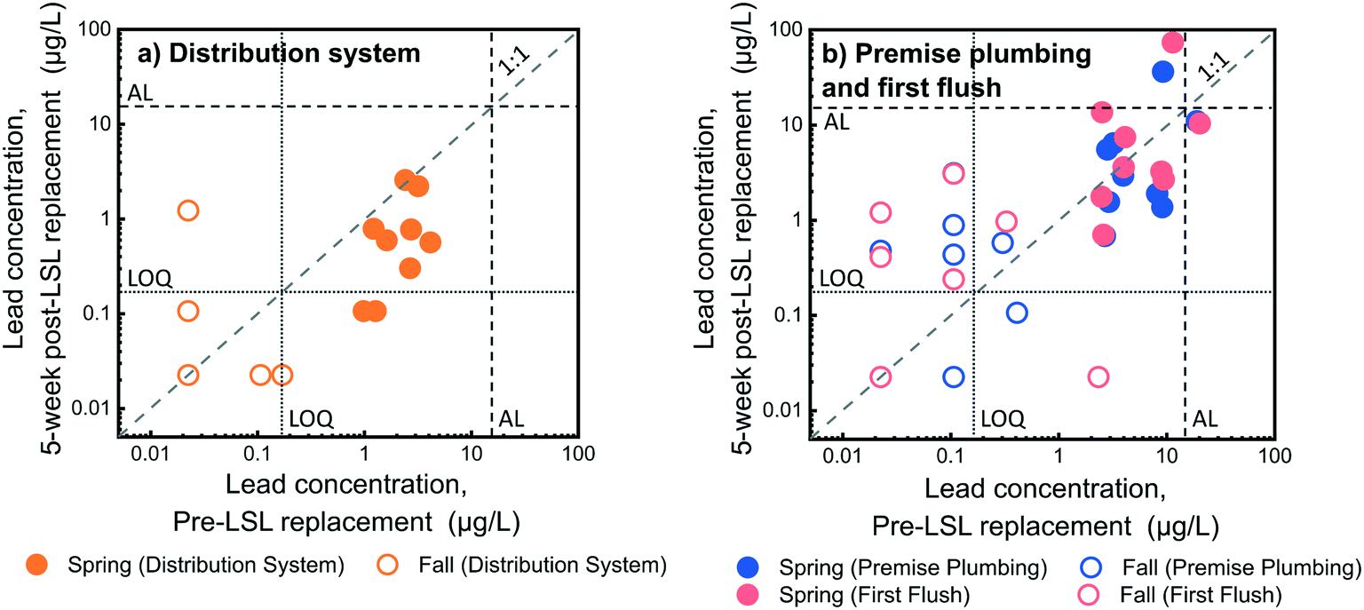

Fig. 1 Lead concentration changes in 17 homes for a) distribution system and b) premise plumbing and first flush samples collected before service line replacement and five weeks after service line replacement in the fall and spring. Dotted horizontal and vertical lines indicate the LOQ. Dashed horizontal and vertical lines indicate the lead action level (AL). Two, two, and five homes were below the LOQ both before and five weeks after service line replacement in first flush, premise plumbing, and distribution system samples, respectively, however not all these samples are visible because of symbol overlap. Raw data is available in ESI† Table S10.

Water lead levels in the first liter, premise plumbing, and hot water samples before service line replacement were not significantly different from two (Wilcoxon signed rank test, p-value = 0.94, 0.59, and 0.79, respectively) or five weeks after service line replacement (Wilcoxon signed rank test, p-value = 1, 0.94, and 0.094, respectively), as shown in Fig. 1b and S4.† Previous studies on the short-term effects of full LSL replacement on water lead level reduction in premise plumbing water are inconsistent. While some studies report almost immediate reductions in lead levels following replacement,¹⁴ others have seen mixed results,³ or only slight reductions.²⁸ These variable short-term LSL replacement outcomes have been attributed to differences in site specific factors, including the materials, water quality, and disturbances at the site.³ Our results support this hypothesis, providing evidence that LSL replacements in a location with recent and significant system-wide disturbances may not result in short-term water lead level reductions in premise plumbing water. When post-LSL replacement samples were collected, no improvement in in-home water lead levels was observed after five weeks, despite the water system in Flint being exposed longer to a corrosion inhibitor. Although no overall improvement was observed in lead levels in the short term, we note that 96% of post-service line replacement samples were below the US EPA lead action level.

A previous study on LSL replacement suggested that the extent of lead seeded in in-home plumbing prior to replacement may determine the time-scale for lead to be flushed from the system.³ This point is important to consider in sites like Flint that have recently undergone extensive corrosion, where leaching of distribution and service line materials likely resulted in widespread seeding of metals in premise plumbing. In these settings, the effects of service line replacement may not be as readily apparent because previously seeded lead continues to persist in water derived from these sources. While our study did not conduct short-term sequential sampling of homes following LSL replacement, 1 L sequential sampling was performed by the US EPA before and after LSL replacement in several Flint homes.¹⁹ Homes were sampled at various times pre- and post-replacement, ranging from the day following replacement to over 35 weeks after replacement. Overall, these data show lead was still present in some premise plumbing sequential samples days to months after LSL replacement.^19,29 The sustained lead concentrations observed in sequential samples representative of the premise plumbing indicate that indeed, lead derived from premise plumbing materials or seeding of premise plumbing materials contributes to the observed premise plumbing water lead levels in the short term.

Comparisons of dissolved and total lead concentrations (Fig. S3†) revealed that more than 93% of all samples contained predominantly particulate lead. Therefore, the persistence of lead in premise plumbing water after LSL replacement must be linked to the fate and sources of particulate lead in the sampled homes. Possible sources include the release of lead-bearing particulates from the service line that accumulated in home plumbing prior to LSL replacement, detachment of particles from premise plumbing surfaces that previously adsorbed dissolved lead from the service line, or the release of particulate lead from corroding fittings or solder in the home that contain lead. Several studies have demonstrated the favorable sorption of lead to iron particles in full- and lab-scale pipe systems,^{4,15,28,30–32} thus they represent a possible source of lead-bearing particulates. A strong positive linear correlation between total lead and iron levels was observed in all sample types (Table S4†) in this study, consistent with earlier findings of significant correlations between particulate lead and iron levels.^{13,14,16,28,33}

The lack of change in water lead levels in premise plumbing samples after service line replacement suggests the five week monitoring period was too short to observe significant improvement. To examine the long-term impact of service line replacement, sequential tap water samples were also collected at a single home (Home 11) with a public LSL and private galvanized service line before and 11 months after service line replacement. Sampling revealed that 11 months after LSL and galvanized service line replacement, lead concentrations were nearly all lower than those before replacement (Fig. 2a).

Fig. 2 a) Total lead and b) total cadmium concentrations collected during service line profiling of 12 sequential 1 L water samples (Home 11). Two profiles were taken pre-service line replacement (red), and two samples were collected approximately 11 months following service line replacement (blue). Gray shading indicates concentrations below the LOQ.

In this home, short-term sampling of premise plumbing displayed water lead levels below the LOQ before service line replacement and two weeks post-service line replacement, while the water lead levels five weeks following replacement was slightly elevated, at 0.43 μg L⁻¹. An estimation of plumbing component volumes at the site indicated the highest lead concentrations before service line replacement were reproducibly drawn from the LSL segment. The majority of post-replacement lead concentrations were below the LOQ, while pre-replacement values were all above the LOQ, with the lowest lead concentration of approximately 1 μg L⁻¹ obtained after flushing.

Integration of the lead masses of the sample profiles revealed that the average mass of lead in the first 12 L decreased by an order of magnitude during the 11 months after service line replacement, from 32.9 to 3.0 μg (Table S6†). Because distribution system water taken at the tap of a home is representative of water being pulled from the water main through the service lines and premise plumbing, the lead levels in this sample type indicate the baseline amount of lead one would expect to find with flushing and high demand from 12 L of water (Fig. S5†). This baseline level of lead in the first 12 L corresponds to 11.5 μg prior to LSL replacement. The sequential sampling profile in Fig. S5† illustrates the impact of overnight stagnation, where the water lead levels are elevated above the baseline by a factor of 3 and 6 in the premise plumbing and the LSL, respectively. Prior to service line replacement, the public service line supplied the majority (57%) of the stagnation contribution to lead mass in the first 12 L. Yet 11 months after replacement, only 4% of the stagnation contribution originated from the service line (Fig. 2). The large contribution of LSLs to lead levels at the tap prior to replacement agrees with work by Sandvig et al., who found LSLs to contribute 50 to 75% of lead to the tap during sequential sampling.³

While lead levels in premise plumbing water across all sampled homes did not decrease significantly within five weeks of service line replacement, the sequential sampling results in Fig. 2a suggest that much lower water lead levels were observed 11 months following service line replacement. Pre-replacement sequential lead profiles in Home 11 were collected about one year after Flint resumed use of Detroit water, and therefore one year after water lead levels began to undergo temporal changes in 2016 as distribution system exposure to corrosion inhibitors proceeded. Some changes in water lead levels pre-LSL replacement compared to 11 months post-LSL replacement could be due to a gradual re-adjustment to water quality changes after the switch back to Detroit water. The reduction in peak lead levels in Fig. 2a pre- and post-LSL replacement, however, are much greater than the reduction in LCR compliance sampling 90th percentiles reported by the City of Flint over the same period, from approximately 12 to 6 μg L⁻¹.^34,35 Our results demonstrate that within a year, LSL replacement can dramatically reduce tap water lead levels. It is important to note that our findings of long-term impacts were only studied in one home, and this is a significant limitation of the study. While we only focused on long-term changes to water lead levels resulting from service line replacement in Home 11, this home's public and private service line configuration (galvanized iron private service line and lead public service line; ESI† Table S1) was the most common configuration for homes in Flint with known public lead service lines.³⁶ To confirm these trends, future longitudinal sampling across multiple homes would need to be performed.

Temporal trends in lead levels from spring to fall 2016

Because homes in this study were sampled during two time periods (spring and fall 2016), an investigation of the temporal variability of water lead levels was feasible. No first flush, premise plumbing, or distribution system samples from the fall 2016 sampling period were above the US EPA lead action level, while 9% (n = 7) of samples from the spring 2016 sampling period were above the action level. Total lead concentrations in pre- and post-SL replacement water samples collected in the fall 2016 sampling period were significantly lower than those collected in spring 2016 (Fig. 3, Wilcoxon rank sum test, p-value = 6.85 × 10⁻¹⁰, 2.15 × 10⁻⁹, and 4.40 × 10⁻⁹ for PP, DS, and hot water samples, respectively). This trend was consistent with the voluntary and sentinel residential drinking water sampling results in Flint in 2016,^37,38 which displayed a significant reduction in lead levels from spring to fall over the same two periods as our sampling study (Wilcoxon rank sum test, p-value < 2.2 × 10⁻¹⁶; n = 6930), with 90th percentile values dropping from 14 μg L⁻¹ to 9 μg L⁻¹ from the spring to fall, respectively. It is important to note that sampling in the volunteer and sentinel studies was conducted city-wide and was not restricted to homes with LSLs, as was the case in our study.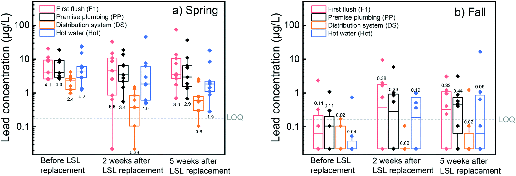

Fig. 3 Median and interquartile range of total lead concentrations collected in a) spring 2016 and b) fall 2016 in first liter (red), premise plumbing (blue), distribution system (yellow), and hot water (black) samples before service line replacement and two and five weeks after service line replacement. Median values are shown above or below each box. The LOQ is indicated by a gray dashed line.

It is generally accepted and has been demonstrated in temporal studies that higher temperatures increase the rate of solubilization and destabilization of particulate lead, resulting in higher lead concentrations in drinking water during warmer seasons.^39–41 Yet our findings display increasing median distribution system temperatures of 9.9 °C during the spring to 17.6 °C during the fall, while the water lead levels decreased between those two periods (Fig. 3). Although temperature may play a role in lead solubilization, our results indicate that there were other factors affecting lead levels in 2016, including known chemistry and physical changes.

Phosphorus levels did not change significantly between spring and fall distribution system samples, however free chlorine levels were higher in the fall than the spring (Wilcoxon rank sum test, p-value = 0.27 and 0.019, respectively). Because lower lead solubility has been observed at elevated free chlorine concentrations,⁴² the increased chlorine residual could contribute to the reduced water lead levels observed in the fall. Increased chlorine concentrations can promote formation of lead(IV) oxides, which have low solubility.⁴³ While formation of these solids may have contributed to the water lead level reductions in Flint during 2016, system complexities make it difficult to predict lead concentrations based on equilibrium assumptions. For example, the evolution of lead(IV) solids in the presence of free chlorine can require time frames of several months.⁴³ Previous equilibrium modeling attempts to predict lead(IV) dissolution have also underpredicted measured lead(IV) concentrations⁴² and the presence of orthophosphate has been shown to complicate lead(IV) release.⁴⁴ We therefore cannot be certain of the extent to which the presence of orthophosphate, increased free chlorine, or both were responsible for the drop in Flint's lower total lead concentrations between spring and fall in 2016. Given the common use of both orthophosphate and free chlorine in drinking water treatment, additional research is needed to better understand their combined impact on lead levels in drinking water.

In addition to chemistry changes, the gradual washout of particulate lead originating from the corrosion episode may also have contributed to the reduced water lead levels in the fall. In May 2016, Flint undertook a flushing campaign. Specifically, Flint residents were encouraged to flush bathtub and kitchen faucets for five minutes every day for 14 days. This campaign could have accelerated the reduction in lead levels that were observed in premise plumbing samples during the fall 2016 sampling period.

Variables affecting total lead levels

Linear mixed-effects models were developed to explain factors influencing total lead concentrations for premise plumbing samples (Table 1) and for distribution system samples (Table S5†), while excluding particulate metal levels that were shown to correlate strongly with total lead levels (Table S4†). In both total lead models, time period was the most significant variable in explaining lead levels. For example, in the premise plumbing lead model (Table 1), spring 2016 samples corresponded to a 1.42 log increase (β) in total lead concentration compared to fall 2016 samples.

Table 1 Results of total lead and dissolved cadmium linear mixed models in premise plumbing samples

	Response variables^a
	log(total lead)			log(dissolved cadmium)
	β	CI	p-Value	β	CI	p-Value
a The slope (β), confidence interval (CI), and p-value of any fixed effects with a significant impact on the response variable are indicated in bold.
Fixed effects
(Intercept)	−0.8	−1.2 to −0.5	3 × 10 ^−5	−1.2	−1.8 to −0.7	6 × 10 ^−4
Percent galvanized PP				0.016	0.008 to 0.023	6 × 10 ^−4
Time period (spring)	1.4	1.0 to 1.8	1 × 10 ^−6	0.3	−0.3 to 1.0	0.3
Visit (two-weeks post-SL replacement)	0.04	−0.3 to 0.4	0.8	−0.4	−0.7 to −0.1	0.02
Visit (five-weeks post-SL replacement)	0.1	−0.3 to 0.4	0.6	−0.6	−0.9 to −0.2	0.001
Random effects		Variance			Variance
Home		0.07			0.3
Observations (n)	51			51

---

The post-service line replacement visits at either two or five weeks were not important in explaining water lead levels in premise plumbing samples. The sequential monitoring experiment suggests that longer term monitoring following service line replacement would have indicated the time of post-service line replacement as an important explanatory variable for describing lead levels.

Cadmium trends in water samples and association with galvanized plumbing

We examined the associations between other metals, and cadmium and zinc concentrations exhibited one of the strongest relationships (Table S4†). Unlike lead, both cadmium and zinc were present primarily as dissolved species (Fig. S6†). The linear correlation between dissolved cadmium and zinc levels, shown in Fig. 4, was driven largely by first liter and premise plumbing samples from three homes (i.e., Homes 2, 7, and 10).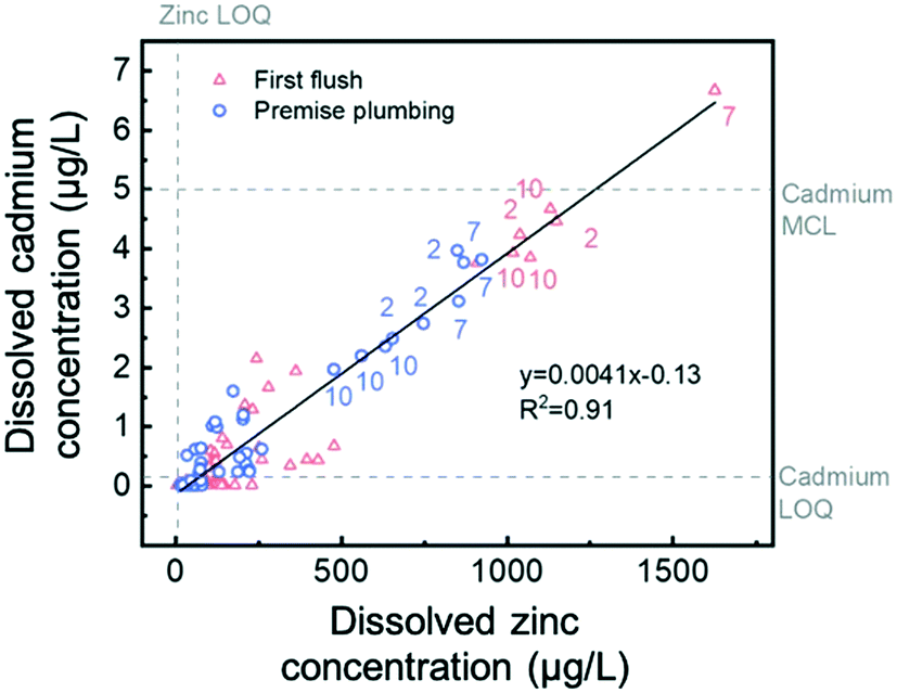

Fig. 4 Relationship between dissolved cadmium and dissolved zinc concentrations for premise plumbing and first liter water samples across 17 homes. Each symbol corresponds to a single sample. Numbers next to symbols refer to a specific home. The best fit linear regression is shown (black line). Gray dashed lines indicate the LOQs for cadmium and zinc, and the maximum contaminant level (MCL) for cadmium.

Samples from these homes were collected in spring 2016 and had cadmium concentrations near or above US EPA's maximum contaminant level (MCL) of 5 μg L⁻¹. Cadmium–zinc associations with sources close to the tap have been reported previously, in particular with galvanized plumbing or brass fixtures.^45–47 The linear fit slope (0.0041 μg L⁻¹ Cd/μg L⁻¹ Zn) in Fig. 4 suggests that cadmium is present on average as a 0.4% impurity in zinc, assuming that zinc and cadmium leach from galvanized or brass surfaces at the same rate. This composition is approximately twice the cadmium content of low grade zinc ore used in galvanizing steel (0.2%).⁴⁸ The elevated Cd/Zn ratio in our study could be due to preferential dissolution of cadmium or brass sources near the tap with elevated Cd/Zn ratios. Brass alloys can contain up to 0.2% cadmium and typically 30% zinc, resulting in a Cd/Zn ratio of 0.0067.⁴⁹

The importance of premise plumbing material was further highlighted through our mixed-effects models, which revealed dissolved cadmium levels were significantly explained by the percentage of galvanized piping in a home's premise plumbing. Overall, this model indicates that a 1% increase in percentage of galvanized premise plumbing corresponds to a 0.02 log increase in cadmium levels (Table 1). Our survey of premise plumbing materials in sampled homes did not include quantification of brass fixtures or fittings, so this variable was not tested in the model and its importance cannot be ruled out.

Short-term impacts of galvanized service line replacement on cadmium levels

We examined the short-term impact of galvanized service line replacement on cadmium levels at the five homes in our study that had private galvanized service lines. Among first flush samples before service line replacement, 6% (n = 1) had total cadmium concentrations above the US EPA's cadmium MCL of 5 μg L⁻¹, while post-replacement 18% (n = 3) of first flush samples had total cadmium concentrations above the MCL. No distribution system or premise plumbing samples were above the MCL either pre- or post-service line replacement. Pairwise comparisons of dissolved cadmium concentrations in individual homes before and up to five weeks after service line replacement are compared in Fig. 5 and S7.†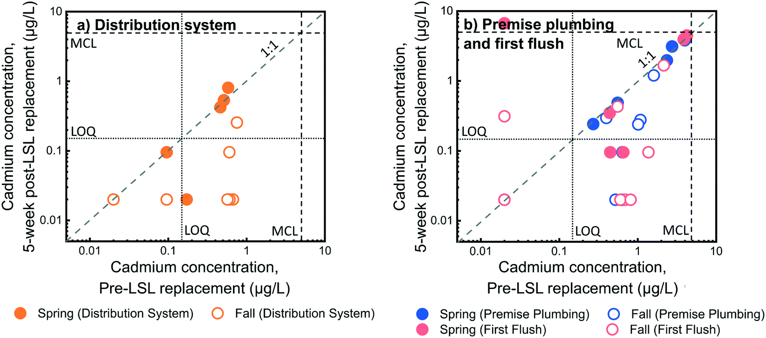

Fig. 5 Dissolved cadmium concentration changes in 17 homes for a) distribution system and b) premise plumbing and first flush samples collected before service line replacement and five weeks after service line replacement in the fall and spring. Dotted horizontal and vertical lines indicate the LOQ. Dashed horizontal and vertical lines indicate the cadmium maximum contaminant level (MCL).

In contrast to the lead response to service line replacement, which did not decrease in first liter or premise plumbing samples within five weeks of replacement, cadmium levels underwent a significant overall reduction in first liter, premise plumbing, and distribution system samples within five weeks of service line replacement (Wilcoxon signed rank test, p-value = 0.0098, 0.0024, and 0.0061 for first liter, premise plumbing, and distribution system samples, respectively). In addition, premise plumbing and distribution samples showed significant reductions just two weeks after replacement (Wilcoxon signed rank test, p-value = 0.10, 2.4 × 10⁻⁴, and 2.4 × 10⁻⁴ for first liter, premise plumbing, and distribution system samples, respectively). The observation that cadmium levels in premise plumbing changed more quickly than lead levels after galvanized service line replacement is not surprising given that cadmium is predominantly present in dissolved form and therefore likely accumulates less in homes relative to particulate lead.

Cadmium levels also decreased in several homes that did not originally have a galvanized service line section (Fig. 5 and S7†). While these homes did not have galvanized service line sections, cadmium has historically been used with zinc to weld seals in lead pipes.⁵⁰ Removal of LSLs could therefore result in reductions of potential cadmium sources even in homes without a private galvanized service line. We suspect that decreases in water temperature could also be responsible for the lower cadmium concentrations observed during return visits to fall 2016 homes, as the median distribution system water temperature decreased from 20.8 °C to 18.7 °C to 15.7 °C during the three sampling visits of fall sampling. Higher temperatures are often linked to faster corrosion rates.⁵¹ Corroboration of the potential effects of temporal water quality changes and service line replacement impact was confirmed through linear mixed-effects modeling results (Table 1). Sampling visit number (visit 1 = pre-replacement, visit 2 = two weeks, and visit 3 = five weeks) correlated significantly with log-transformed dissolved cadmium levels. Specifically, the two-week post-service line replacement visit marked a 0.41 log reduction (p-value = 0.016) in cadmium levels over the pre-service line replacement visit and the five-week post-service line replacement visit followed a similar trend (β = −0.56, p-value = 0.001).

Long-term impacts of service line replacement on cadmium levels

Long-term changes in cadmium levels after service line replacement were also examined by sequential sampling at Home 11 (Fig. 2b). This home had a private galvanized service line and premise plumbing that was approximately 81% galvanized material by length. Prior to service line replacement, integration of cadmium concentrations over the volume of each pipe segment (Table S7†) revealed approximately 10.9 μg of cadmium was released in the first 12 L of water sampled. Prior to service line replacement, the lowest cadmium concentration observed was approximately 0.7 μg L⁻¹ Cd (with flushing), suggesting there was a measurable baseline concentration in all tap water samples without stagnation (or a baseline mass of approximately 8.6 μg Cd in 12 L). Overnight stagnation in the premise plumbing and galvanized service line segments contributed an additional 1.0 and 1.1 μg Cd, respectively, above the baseline (total 10.9 μg of Cd in 12 L). Before service line replacement, the premise plumbing and galvanized service line contributed equally to the additional cadmium mass due to stagnation, which may be a result of the high percentage of galvanized plumbing in the home. Overnight stagnation, however, caused less of a fractional increase (21%) over the baseline cadmium mass than that observed for lead (65%).

Eleven months after service line replacement, cadmium levels in most of the profile samples fell below quantification limits, with the exception of a couple premise plumbing samples as shown in Fig. 2b. The large reduction in premise plumbing cadmium concentrations relative to pre-galvanized service line replacement values is perhaps unexpected, given that plumbing in the home was still predominantly galvanized. We note, however, that cadmium concentrations in premise plumbing were between the LOQ (0.15 μg L⁻¹) and the LOD (0.04 μg L⁻¹), while the service line sample concentrations were all below the LOD. The decrease in premise plumbing cadmium concentrations after galvanized service line replacement could be due to the loss of cadmium that accumulated in the home from the upstream galvanized service line or the longer exposure of premise plumbing to DWSD water and consequently corrosion inhibitor. The pre-service line replacement premise plumbing sample taken in August 2016 for Home 11 had a cadmium concentration of 1.05 μg L⁻¹, which agrees with the average cadmium concentration found in the first 3 L of sequential samples from Home 11 in September 2016, 0.98 μg L⁻¹. Distribution system samples also showed similar results between the pre-service line sample and the first 3 L of sequential samples, with cadmium levels of 0.79 μg L⁻¹ and 0.71 μg L⁻¹, respectively.

Temporal patterns for dissolved cadmium levels in the first liter and premise plumbing samples suggest a greater variation in levels and larger maximum values in spring 2016 compared to fall 2016, as illustrated in Fig. 6.

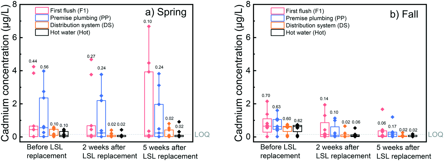Fig. 6 Median and interquartile ranges of dissolved cadmium concentrations collected in a) spring 2016 and b) fall 2016 in samples before SL replacement and two and five weeks after SL replacement. Median values are shown above each box. The LOQ is indicated by a gray dashed line.

Mixed-effects models of the log transformed median dissolved cadmium levels, however, were not significantly explained by the temporal sampling period (spring versus fall). These results suggest the maximum cadmium concentrations decreased upon longer exposure to DWSD water, but median levels were not significantly affected.

Temporal trends from spring to fall 2016 in total bacteria and select opportunistic pathogen abundance in water samples

We quantified gene copy levels of total bacteria, Mycobacterium spp., Legionella spp., and L. pneumophila in water samples to determine whether opportunistic pathogens could have been a concern in homes during the sampling time frame. All samples had quantifiable concentrations of total bacteria, while 21% and 52% of samples had Legionella spp. and Mycobacterium spp. concentrations above the LOQ, respectively. No water samples contained detectable L. pneumophila gene copies. Given the high level of interest in bacterial abundance in Flint's water distribution system, we have archived details of bacterial analyses and trends in the ESI† without further discussion here.

Conclusions

At short time scales (i.e., less than five weeks), no significant impact of service line replacement on first liter and premise plumbing sample lead concentrations was observed in Flint homes. However, short-term reductions in lead were observed in samples drawn from the distribution system by flushing after service line replacement. Based on sequential sampling, dramatic improvements in water lead levels were observed in all of the first 12 L samples 11 months post-service line replacement, suggesting the valuable long-term benefits of this lead mitigation strategy. This trend, however, was only identified in one home in this study, and future work should focus on confirming these findings with a larger subset of homes. The longer delays in premise plumbing lead reductions observed in this study may be due to a greater accumulation of lead in home plumbing and greater instability of premise plumbing scale after Flint's corrosion episode. Consumers in households with a replaced LSL, therefore, should be advised to continue lead mitigation strategies (e.g., point-of-use filters and/or flushing after stagnation periods) for several months after LSL replacement to fully minimize their lead exposure, although the precise timeline necessary is unclear. More research is needed to determine exactly how long the seeded in-home lead sources may continue to leach into drinking water, with particular focus on how the degree of seeding in premise plumbing may affect this time-frame.

This work provides information for the ongoing discussion of whether LSL replacement is an effective lead mitigation strategy in the short term, due to its high cost compared to other short-term strategies.⁵² Our work indicates that short-term reductions in water lead levels following LSL replacement may not be observed in regions where extensive seeding of lead in in-home plumbing has occurred; however, the beneficial removal of lead sources in the long term is evident from this work as well as from other recent work.²⁰ These findings must be carefully weighed by utilities and regulators in determining what is best for a community to recover and provide a reliable, safe source of drinking water.

In addition to the benefit of replacing service lines for lead level reduction, our results highlight the benefits of removing service lines as part of replacement programs for reduction of cadmium levels in drinking water. While the role of galvanized service lines as a source of lead exposure through their sorptive capacity and potential for lead release have been well documented,¹⁰ our findings show that service lines and galvanized premise plumbing can represent an important source of cadmium. Under corrosive water conditions, water levels of cadmium in galvanized plumbing may exceed US EPA's MCL of 5 μg L⁻¹. After LSL and galvanized service line replacement in Flint, cadmium concentrations were significantly reduced within five weeks in first liter, premise plumbing, and distribution system samples and were below method quantification limits in any of the first 12 L samples of one home after 11 months. Given that cadmium has not been part of the lead and copper rule monitoring program,²¹ fewer data are available on its occurrence and response to water quality changes in the distribution system compared to lead and copper. Unlike lead, cadmium is largely present in the dissolved state and cadmium concentrations might be expected to respond more quickly to water quality changes. Therefore, additional study and monitoring of cadmium in drinking water should be conducted as utilities seek to optimize their corrosion control strategies.

Conflicts of interest

The authors declare no conflicts of interest.

Acknowledgements

This work was funded by the University of Michigan (UM) MCubed program. NCR was partially supported by a U.S. National Science Foundation Graduate Research Fellowship (award no. 2015205675), and YS and SJH were supported by Alfred P. Sloan Foundation Microbiology of the Built Environment Fellowships (G-2016-7250 and G-2014-13739, respectively). Additionally, SJH was supported by a UM Dow Sustainability Fellowship. The sponsors had no role in study design, data collection, interpretation, or the decision to submit this work for publication. We thank UM Flint faculty, Marty Kaufman, UM Flint GIS Center Manager, and Troy Rosencrants, and UM Flint students Zachary Hayes, David Yeoman, Brandon Eggleston, Brie Warner, and Catherine Wilhelm for contributions to sampling and sample processing, and the FAST Start program coordinator, retired Brigadier General Michael McDaniel, and his team for their coordination and aid in pipe sample collection. Additionally, we thank UM Ann Arbor student Guy Burke for sample processing and metals analyses and Michele Swanson's laboratory for the L. pneumophila strain Lp02 DNA extract. Finally, we are grateful to the residents of Flint, who allowed us to sample and survey their homes.

References

1. World Heatlh Organization, Lead in Drinking-water, Geneva, 2011.
2. D. A. Cornwell, R. A. Brown and S. H. Via, National Survey of Lead Service Line Occurrence, J. - Am. Water Works Assoc., 2016, 108, 87.
3. A. Sandvig, P. Kwan, G. Kirmeyer, B. Maynard, D. Mast, R. R. Trussell, R. S. Trussell, A. F. Cantor and A. Prescott, Contribution of Service Line and Plumbing Fixtures to Lead and Copper Rule Compliance Issues, AWWA Res. Found., 2010.
4. B. F. Trueman and G. A. Gagnon, Understanding the Role of Particulate Iron in Lead Release to Drinking Water, Environ. Sci. Technol., 2016, 50, 9053–9060.
5. E. Deshommes, B. Trueman, I. Douglas, D. Huggins, L. Laroche, J. Swertfeger, A. Spielmacher, G. A. Gagnon and M. Prévost, Lead Levels at the Tap and Consumer Exposure from Legacy and Recent Lead Service Line Replacements in Six Utilities, Environ. Sci. Technol., 2018, 52, 9451–9459.
6. P. Levallois, J. St-Laurent, D. Gauvin, M. Courteau, M. Prévost, C. Campagna, F. Lemieux, S. Nour, M. D'Amour and P. E. Rasmussen, The impact of drinking water, indoor dust and paint on blood lead levels of children aged 1-5 years in Montréal (Québec, Canada), J. Exposure Sci. Environ. Epidemiol., 2014, 24, 185–191.
7. S. Zahran, S. P. McElmurry and R. C. Sadler, Four phases of the Flint Water Crisis: Evidence from blood lead levels in children, Environ. Res., 2017, 157, 160–172.
8. M. Hanna-Attisha, J. LaChance, R. C. Sadler and A. Champney Schnepp, Elevated Blood Lead Levels in Children Associated With the Flint Drinking Water Crisis: A Spatial Analysis of Risk and Public Health Response, Am. J. Public Health, 2015, 106, 283–290.
9. C. Kennedy, E. Yard, T. Dignam, S. Buchanan, S. Condon, M. J. Brown, J. Raymond, H. S. Rogers, J. Sarisky, R. de Castro, I. Arias and P. Breysse, Blood Lead Levels Among Children Aged <6 Years - Flint, Michigan, 2013-2016, Morb. Mortal. Wkly. Rep., 2016, 65, 650–654.
10. K. J. Pieper, M. Tang and M. A. Edwards, Flint Water Crisis Caused By Interrupted Corrosion Control: Investigating “Ground Zero” Home, Environ. Sci. Technol., 2017, 51, 2007–2014.
11. T. M. Olson, M. Wax, J. Yonts, K. Heidecorn, S.-J. Haig, D. Yeoman, Z. Hayes, L. Raskin and B. R. Ellis, Forensic Estimates of Lead Release from Lead Service Lines during the Water Crisis in Flint, Michigan, Environ. Sci. Technol. Lett., 2017, 4, 356–361.
12. P. Goovaerts, The drinking water contamination crisis in Flint: Modeling temporal trends of lead level since returning to Detroit water system, Sci. Total Environ., 2017, 581, 66–79.
13. K. J. Pieper, R. Martin, M. Tang, L. Walters, J. Parks, S. Roy, C. Devine and M. A. Edwards, Evaluating Water Lead Levels During the Flint Water Crisis, Environ. Sci. Technol., 2018, 52, 8124–8132.
14. B. F. Trueman, E. Camara and G. A. Gagnon, Evaluating the Effects of Full and Partial Lead Service Line Replacement on Lead Levels in Drinking Water, Environ. Sci. Technol., 2016, 50, 7389–7396.
15. E. Camara, K. Montreuil, A. Knowles and G. A. Gagnon, Role of the water main in lead service line replacement: A utility case study, J. - Am. Water Works Assoc., 2013, 105, E423–E431.
16. E. Deshommes, L. Laroche, D. Deveau, S. Nour and M. Prévost, Short- and Long-Term Lead Release after Partial Lead Service Line Replacements in a Metropolitan Water Distribution System, Environ. Sci. Technol., 2017, 51, 9507–9515.
17. G. R. Boyd, P. Shetty, A. M. Sandvig and G. L. Pierson, Pb in Tap Water Following Simulated Partial Lead Pipe Replacements, J. Environ. Eng., 2004, 130, 1188–1197.
18. J. St. Clair, C. Cartier, S. Triantafyllidou, B. Clark and M. Edwards, Long-Term Behavior of Simulated Partial Lead Service Line Replacements, Environ. Eng. Sci., 2016, 33, 53–64.
19. D. A. Lytle, M. R. Schock, K. Wait, K. Cahalan, V. Bosscher, A. Porter and M. Del Toral, Sequential drinking water sampling as a tool for evaluating lead in flint, Michigan, Water Res., 2019, 157, 40–54.
20. A. Mantha, M. Tang, K. J. Pieper, J. L. Parks and M. A. Edwards, Tracking reduction of water lead levels in two homes during the Flint Federal Emergency, Water Res.: X, 2020, 7, 100047.
21. U.S. Environmental Protection Agency, National Primary Drinking Water Regulations, 40 CFR Part 141 Subpart 1, 1991.
22. W. J. Rhoads, E. Garner, P. Ji, N. Zhu, J. Parks, D. O. Schwake, A. Pruden and M. A. Edwards, Distribution System Operational Deficiencies Coincide with Reported Legionnaires’ Disease Clusters in Flint, Michigan, Environ. Sci. Technol., 2017, 51, 11986–11995.
23. D. O. Schwake, E. Garner, O. R. Strom, A. Pruden and M. A. Edwards, Legionella DNA Markers in Tap Water Coincident with a Spike in Legionnaires’ Disease in Flint, MI, Environ. Sci. Technol. Lett., 2016, 3, 311–315.
24. S. Zahran, S. P. McElmurry, P. E. Kilgore, D. Mushinski, J. Press, N. G. Love, R. C. Sadler and M. S. Swanson, Assessment of the Legionnaires’ disease outbreak in Flint, Michigan, Proc. Natl. Acad. Sci. U. S. A., 2018, 115, E1730–E1739.
25. R Core Team, R: A Language and Environment for Statistical Computing, 2020.
26. T. Hothorn and K. Hornik, Exact Distributions for Rank and Permutation Tests, 2017.
27. W. Revelle, psych: Procedures for Psychological, Psychometric, and Personality Research, 2020.
28. M. McFadden, R. Giani, P. Kwan and S. H. Reiber, Contributions to drinking water lead from galvanized iron corrosion scales, J. - Am. Water Works Assoc., 2011, 103, 76–89.
29. U.S. Environmental Protection Agency, 2020.
30. S. Masters and M. Edwards, Increased Lead in Water Associated with Iron Corrosion, Environ. Eng. Sci., 2015, 32, 361–369.
31. M. Schock, A. F. Cantor, S. Triantafyllidou, M. Desantis and K. Scheckel, Importance of pipe deposits to Lead and Copper Rule compliance, J. - Am. Water Works Assoc., 2014, 106, E336–E349.
32. A. S. Hill, M. J. Friedman, S. H. Reiber, G. V. Korshin and R. L. Valentine, Behavior of Trace Inorganic Contaminants in Drinking Water Distribution Systems, J. - Am. Water Works Assoc., 2010, 102, 107–118.
33. B. Clark, S. Masters and M. Edwards, Profile Sampling To Characterize Particulate Lead Risks in Potable Water, Environ. Sci. Technol., 2014, 48, 6836–6843.
34. City of Flint 2016 Annual Water Quality Report, Flint, MI, 2016.
35. City of Flint 2017 Annual Water Quality Report, Flint, MI, 2017.
36. J. Abernethy, A. Chojnacki, A. Farahi, E. Schwartz and J. Webb, in Proceedings of the 24th ACM SIGKDD International Conference on knowledge discovery & data mining, ACM, 2018, pp. 5–14.
37. Michigan, Taking Action on Flint Water: Residential Sampling, https://www.michigan.gov/flintwater/0,6092,7-345-76292_76294_76297---,00.html, (accessed 7 July 2018).
38. Michigan, Taking Action on Flint Water: Sentinel/LCR Sampling.
39. S. Masters, G. J. Welter and M. Edwards, Seasonal Variations in Lead Release to Potable Water, Environ. Sci. Technol., 2016, 50, 5269–5277.
40. P. C. Karalekas Jr., C. R. Ryan and F. B. Taylor, Control of lead, copper, and iron pipe corrosion in Boston, J. - Am. Water Works Assoc., 1983, 75, 92–95.
41. E. Deshommes, M. Prévost, P. Levallois, F. Lemieux and S. Nour, Application of lead monitoring results to predict 0–7 year old children's exposure at the tap, Water Res., 2013, 47, 2409–2420.
42. Y. Xie, Y. Wang and D. E. Giammar, Impact of Chlorine Disinfectants on Dissolution of the Lead Corrosion Product PbO2, Environ. Sci. Technol., 2010, 44, 7082–7088.
43. D. A. Lytle and M. R. Schock, Formation of Pb(IV) oxides in chlorinated water, J. - Am. Water Works Assoc., 2005, 97, 102–114.
44. G. Korshin and H. Liu, Preventing the colloidal dispersion of Pb(iv) corrosion scales and lead release in drinking water distribution systems, Environ. Sci.: Water Res. Technol., 2019, 5, 1262–1269.
45. B. P. Zietz, K. Richter, J. Laß, R. Suchenwirth and R. Huppmann, Release of Metals from Different Sections of Domestic Drinking Water Installations, Water Qual., Exposure Health, 2015, 7, 193–204.
46. A. R. Sharrett, A. P. Carter, R. M. Orheimt and M. Feinleib, Daily Intake of Lead, Cadmium, Copper, and Zinc from Drinking Water: the Seattle Study of Trace Metal Exposure, Environ. Res., 1982, 28, 456–475.
47. B. N. Clark, S. V. Masters and M. A. Edwards, Lead Release to Drinking Water from Galvanized Steel Pipe Coatings, Environ. Eng. Sci., 2015, 32, 713–721.
48. S. Gonzalez, R. Lopez-Roldan and J.-L. Cortina, Presence of metals in drinking water distribution networks due to pipe material leaching: a review, Toxicol. Environ. Chem., 2013, 95, 870–889.
49. A. T. Etheridge, The estimation of cadmium in brass, Analyst, 1924, 49, 572–576.
50. R. A. Bernhoft, Cadmium toxicity and treatment, Sci. World J., 2013, 2013, 394652.
51. Y. Lee, Asian J. Chem., 2008, 20, 6535–6550.
52. S. J. Masten, S. H. Davies, S. W. Haider and C. R. McPherson, Reflections on the Lead and Copper Rule and Lead Levels in Flint's Water, J. - Am. Water Works Assoc., 2019, 111, 42–55.

---

Footnotes

† Electronic supplementary information (ESI) available. See DOI: 10.1039/d0ew00975j

‡ Current affiliation: Department of Chemical and Environmental Engineering, University of California, Riverside, Riverside, CA.

§ Current affiliation: Department of Civil and Environmental Engineering, University of Pittsburgh, Pittsburgh, PA.

¶ Current affiliation: Jacobs, Bingham Farms, Michigan.

|| Current affiliation: Tetra Tech, Inc., Lansing, Michigan.

---