
 Open Access Article
 This Open Access Article is licensed under a
 Creative Commons Attribution 3.0 Unported Licence
Spatiotemporal profiles of ultrafine particles differ from other traffic-related air pollutants: lessons from long-term measurements at fixed sites and mobile monitoring†
Shahzad
Gani‡
 *ab,
Sarah E.
Chambliss‡
c,
Kyle P.
Messier
d,
Melissa M.
Lunden
e and
Joshua S.
Apte
fg
*ab,
Sarah E.
Chambliss‡
c,
Kyle P.
Messier
d,
Melissa M.
Lunden
e and
Joshua S.
Apte
fg
aInstitute of Atmospheric and Earth System Sciences/Physics, University of Helsinki, Finland. E-mail: shahzad.gani@helsinki.fi
bHelsinki Institute of Sustainability Science, University of Helsinki, Helsinki, Finland
cDepartment of Statistics and Data Sciences, University of Texas at Austin, Texas, USA
dDivision of the National Toxicology Program, National Institute of Environmental Health Sciences, Durham, North Carolina, USA
eAclima, Inc., San Francisco, California, USA
fDepartment of Civil and Environmental Engineering, University of California, Berkeley, California, USA
gSchool of Public Health, University of California, Berkeley, California, USA
First published on 14th October 2021
Abstract
In the absence of routine monitoring of ultrafine particles (UFP, Dp < 100 nm), air pollution epidemiology studies often use other co-emitted pollutants as a proxy for UFP, with NOx (NO + NO2) considered a good choice. We use long term fixed site measurements along with extensive mobile monitoring data to evaluate the spatiotemporal correlation of UFP and NOx. We incorporate 6 years of hourly particle number (PN, an approximation of UFP) concentration data from multiple fixed sites across the San Francisco Bay Area that include near-highway, urban, suburban, and rural sites. In addition, we incorporate observations from a 32 month mobile monitoring campaign comprising >1000 h of coverage of a range of road types and land uses. Across all fixed sites, PN concentrations show prominent mid-day peaks during the summer – characteristic of new particle formation – which are not observed for other co-emitted pollutants (NOx, BC, CO). While we find moderate correlation in diurnal patterns of NOx and UFP at sites with high traffic, the correlation drops significantly for low traffic areas, especially during high insolation (e.g., summer daytime) periods. Mobile monitoring data yields similar results: NOx is observed to have weaker correlation with PN for non-highway roads during high insolation periods. The spatiotemporal profiles of UFP can differ strongly from other co-emitted air pollutants when new particle formation contributes a significant share of UFP.
Environmental significanceAlthough particle number (PN) is theorized to be more strongly linked with adverse health effects than total particle mass, difficulty in producing an accurate characterization of spatial variation of PN in urban areas remains an impediment to evaluating its health effects. Long-term fixed-site measurements and extensive mobile monitoring data show complementary evidence that elevated summertime PN concentrations, arising from new particle formation, follow spatial and temporal patterns that diverge from those of other traffic-related air pollutants such as NOx and black carbon. Seasonal PN–NOx decoupling was especially pronounced in residential areas, which are less influenced by vehicle emissions. These findings indicate the importance of considering complex atmospheric processes along with key emission sources (i.e., traffic) in models of ultrafine particle exposure and strategies for reducing ambient ultrafine particle levels. |
1 Introduction
Recent studies show that air pollution may be damaging to almost every organ in the human body.1,2 Ultrafine particles (UFP), aerosol particles with aerodynamic diameter <100 nm, are known to penetrate deep within the lungs and may enter the bloodstream and reach sensitive internal organs.3,4 Furthermore, unlike larger particles, UFP can be deposited into the brain, causing adverse cognitive effects.5–7 While consensus on the health effects of UFP, separate from fine particulate matter (PM2.5), is yet to be reached,8 there has been an increase in studies linking UFP exposure to cell damage, adverse cardiovascular health effects, and the formation of certain cancers (e.g., brain cancers).5,9–13Due to these health risks, population exposure to UFP is the subject of current investigation in air pollution epidemiology.14 However, UFP exposure is difficult to characterize due to the high variability in UFP concentrations over short temporal and spatial scales. As with many air pollutants emitted in urban areas, patterns of UFP are spatiotemporally complex: spatial patterns vary over time, and temporal patterns vary in space. However, there are few networks around the world that routinely measure UFP concentrations, typically with a small number of continuous monitors,15–17 which are not capable of resolving the spatiotemporal dynamics of UFP across the urban landscape. Accordingly, health studies employ a range of alternative strategies for estimating spatial patterns of UFP exposure, including short-term distributed sampling, regional scale-air quality modeling, and land-use regression models based on short-term measurements.18,19 In urban areas the principal sources of UFP include vehicular traffic (tailpipe emissions, brake wear, and tire wear), other combustion of fossil fuels, cooking, and nucleation events.20–23 Because traffic is often assumed to be a dominant source of UFP, exposure to UFP is sometimes approximated based on more commonly observed traffic-related air pollutants (commonly NOx or NO2) as indicator values.24–29 However, the strength of correlation between UFP and other traffic-related air pollutants (TRAPs, including NO, NO2, CO, and BC) varies among sites.30–35 In this study we examine conditions under which the spatiotemporal signatures of UFP may differ meaningfully from those of other TRAPs.
Spatiotemporal variation of UFP is influenced by a complex interplay between local sources, long-range sources, meteorological conditions, and aerosol dynamic processes.36,37 Unlike other TRAPs, UFP concentrations are strongly affected by regional new particle formation (NPF) from atmospheric vapors. NPF events have been observed in urban, regional, and background environments.37–44 In recent years, studies from various cities and background sites across the world show particle number (PN) concentrations, which are dominated by the ultrafine particle number count, peak during periods with increased solar radiation.16,45–54 Short term studies that have investigated both particle formation and growth have found NPF to be an important contributor to overall UFP concentrations.55–58 Brines et al.21 studied multiple cities in the Mediterranean climatic regions (Barcelona, Madrid, Rome and Los Angeles) and found that although traffic remains the main source of UFP in urban areas, during high insolation (sunny) periods, NPF can become the main source of UFP. Under these conditions UFP concentrations can become decoupled from TRAP concentrations, which are driven primarily by emissions activity. However, most observational comparisons between UFP and other TRAPs are generally based on short-term mobile or distributed-sampler studies,18,19,59–63 usually not capable of comprehensively characterizing seasonal patterns.
Here, we combine two unique long-term observational datasets of particle number (PN) concentrations from the San Francisco Bay Area (USA) to investigate the spatial and temporal variation of ultrafine particulate matter. We consider multiple spatial scales – from fine-scale variation within neighborhoods to a broad rural-to-urban gradient – and investigate temporal variation at the diurnal and seasonal scales. Through these observations, we highlight conditions where UFP patterns show substantial deviation from those of other traffic-related air pollutants, likely resulting in a health-relevant divergence in patterns of exposure.
2 Materials and methods
This study combines long-term fixed site measurements and on-road mobile monitoring measurements in the San Francisco (SF) Bay Area, California, USA. The SF Bay Area climate is temperate, with moderate winters and summers in the coastal areas and warm summer days in the inland valleys. Representative seasonal and diurnal profiles of key meteorological parameters are presented in the ESI (Fig. S1†). The fixed sites and mobile monitoring measurements were spread across environments representing the varying levels of urbanization, traffic activity and composition, and other urban emissions activity.2.1 Fixed sites
We incorporate hourly pollution monitoring data collected at four fixed sites in the Bay Area Air Quality Management District's monitoring network over a period of 4–6 years (Jul-2011–Jan-2018).64 The chosen sites represent different land uses and emissions intensity levels for the San Francisco Bay Area, including near-highway (Laney College), urban (Redwood City), suburban (Livermore), and rural (Sebastopol) sites. PN and NOx were measured at each of these four sites, CO at three sites (near-highway, urban, and rural), and BC at two sites (near-highway and suburban). Details of fixed sites (measurement period, pollutants measured, distance from nearest highway, and their location on a map) are presented in the ESI (Table S1 and Fig. S2†). For the fixed sites, PN concentrations were measured using condensation particle counters (CPC, TSI, model 3783, Dp > 7 nm). NOx was measured using chemiluminescence analyzers (Thermo Scientific, model 42i). Black Carbon (BC) and Carbon Monoxide (CO) were measured using aethalometers (Teledyne, model 633, equivalent to a Magee Scientific model AE33) and gas filter correlation CO analyzers (Thermo Scientific, model 48i) respectively. We use data from 2015 (year with almost full coverage for measured pollutants at all sites) for calculating the annual average (Section 3.1). However, unless stated otherwise, we use all available hourly data (4–6 years) from the fixed sites for the analyses presented in this study. For our analysis we define daytime as 8 am–8 pm and nighttime as 8 pm–8 am. We define summer as the first day of June through the final day of August and winter as the first day of December through the final day of February.2.2 Mobile monitoring
To investigate time-stable trends with higher spatial resolution, we incorporate observations from a 32 month mobile monitoring campaign in the SF Bay Area65 using two Google Street View cars equipped with the Aclima mobile measurement and data acquisition platform outfitted with research grade equipment (Aclima Inc., San Francisco CA). To allow for a comparison of patterns by season, this analysis focuses on the portions of the driving domain most extensively sampled during the campaign: Downtown Oakland and West Oakland neighborhoods. West Oakland is comprised of low- and mid-rise residential/commercial neighborhoods, numerous small and mid-sized industries and warehouses, is adjacent to a port, and is surrounded by major highways. Downtown Oakland has mixed residential and commercial zoning with mid- and high-rise construction. Overall, we collected ∼1125 hours of mobile monitoring data on 50 kilometers of roads within these two neighborhoods, with a range of 1–133 repeated visits to each road segment on 1–54 unique days over this 32 month period (May-2015–May-2017). The mobile monitoring campaign employed fast response lab-grade instruments. Ultrafine particles were measured using CPCs (TSI, model 3788, Dp > 2.5 nm), NO using chemiluminescence (Model CLD64, Eco Physics AG, Switzerland), and NO2 was measured using cavity-attenuation phase-shift spectroscopy (Model T500U, Teledyne Inc., San Diego, CA). The CPCs used for mobile monitoring campaign had a cut point of 2.5 nm, compared to the 7 nm cut point of the fixed sites CPCs (we do not compare concentrations between fixed sites and mobile monitoring in this study). The mobile monitoring platforms had separate inlets for particle and gas measurements, with particle inlets designed to minimize diffusional sampling losses. To minimize the influence of self-emissions on the measured pollutant concentrations, these collocated inlets were positioned in a forward-facing orientation several inches above the roof line at the rear edge of the front window of the cars. Details of the mobile monitoring setup have been presented in Apte et al.65 and its ESI.†Data processing for mobile monitoring followed the steps described in Messier et al.:66 road line geometry data for the San Francisco Bay Area were obtained from OpenStreetMaps (OSM) and converted to point geometry at 30 m spacing, corresponding to the midpoint of individual 30 m road segments. Each measured 1 Hz data point was ‘snapped’ to the coordinates of the nearest road segment. Data were collected at >1600 total road segments in West and Downtown Oakland, California. The road segments were designated as ‘highway’, ‘arterial’, or ‘residential’ road data based on OSM classification codes. For seasonal or long-term spatial patterns, an additional data reduction technique was applied to ensure that each repeated drive through a given road segment (drive pass) was represented equally.66 First, measurements for each ‘drive pass’ were reduced into a single drive pass mean concentration value. The median of drive pass means at each road segment was used as the core metric for mobile monitoring spatial analyses. These analyses exclude road segments with data from fewer than 5 sampling days as the small sample size limits statistical confidence in concentration estimates at those locations. For logistical reasons, mobile measurements were restricted to weekday and daytime conditions. Given the aforementioned sample-size considerations, the mobile measurements are capable of resolving seasonal-average spatial patterns for typical daytime conditions, but lack the granular temporal resolution of continuous fixed-site measurements. Accordingly, our mobile measurements capture the seasonal aspects of spatiotemporal variability, but do not reflect the marked difference in TRAP spatial patterns that occur between day and night that have been identified by prior mobile transect studies.67
2.3 Supplementary datasets
We use mesoscale (regional) meteorological data for wind speed (10 m from ground) and planetary boundary layer height (PBLH) to calculate the regional-scale ventilation coefficient (VC = wind speed × PBLH). These data for the SF Bay area were obtained from NASA's meteorological reanalysis dataset, MERRA2.68 MERRA2 has a spatial resolution of 0.5° × 0.625° (55 km × 60 km) and an hourly temporal resolution. Given the large area covered in a single MERRA2 grid, the grid we chose covered most of the sites including the near-highway, urban, and suburban site.For the near-highway site, we obtained traffic data (vehicular and truck flow) from the Freeway Performance Measurement System maintained by the California Department of Transportation.69 We chose the traffic sensor closest to our near-highway fixed site (Mainline VDS 400218). Both the traffic sensor and the fixed site were adjacent to highway I880-N. For our analysis, we used hourly traffic data for 2015 and monthly data for 2014–2018.
3 Results and discussion
3.1 Temporal variation of TRAP concentrations
Among the fixed sites, TRAP concentrations were highest for the near-highway site, followed by the urban, suburban, and rural sites, consistent with patterns observed in other areas.70 For 2015 (year with almost full coverage for measured pollutants at all sites), from near-highway to rural, the annual average (5th–95th percentile) PN concentrations were 29![[thin space (1/6-em)]](https://www.rsc.org/images/entities/char_2009.gif) 900 cm−3 (7960–65500 cm−3), 11900 cm−3 (1850–31100 cm−3), 10100 cm−3 (1990–21100 cm−3), and 3500 cm−3 (430–10500 cm−3) respectively. Annual average NOx concentrations followed the same order – 34.7 ppb (7.1–87.7 ppb) for the near-highway, 18.8 ppb (2.3–61.1 ppb) for the urban, 17.4 ppb (1.9–63.4 ppb) for the suburban, and 8.4 ppb (1.2–28.6 ppb) for the rural site. Among these sites, BC was only monitored at the near-highway and the suburban sites for which the annual average concentrations were 1.43 μg m−3 (0.28–3.65 μg m−3) and 0.78 μg m−3 (0.09–2.61 μg m−3) respectively. CO annual average concentrations were 0.47 ppm (0.25–0.86 ppm) at the near-highway site, 0.44 ppm (0.23–0.92 ppm) at the urban site, and 0.38 ppm (0.20–0.66 ppm) at the rural site. The low CO concentrations and the small differences among sites are consistent with the large reductions in vehicular CO emissions (∼80–90%) over the last few decades in urban areas in the US.71
900 cm−3 (7960–65500 cm−3), 11900 cm−3 (1850–31100 cm−3), 10100 cm−3 (1990–21100 cm−3), and 3500 cm−3 (430–10500 cm−3) respectively. Annual average NOx concentrations followed the same order – 34.7 ppb (7.1–87.7 ppb) for the near-highway, 18.8 ppb (2.3–61.1 ppb) for the urban, 17.4 ppb (1.9–63.4 ppb) for the suburban, and 8.4 ppb (1.2–28.6 ppb) for the rural site. Among these sites, BC was only monitored at the near-highway and the suburban sites for which the annual average concentrations were 1.43 μg m−3 (0.28–3.65 μg m−3) and 0.78 μg m−3 (0.09–2.61 μg m−3) respectively. CO annual average concentrations were 0.47 ppm (0.25–0.86 ppm) at the near-highway site, 0.44 ppm (0.23–0.92 ppm) at the urban site, and 0.38 ppm (0.20–0.66 ppm) at the rural site. The low CO concentrations and the small differences among sites are consistent with the large reductions in vehicular CO emissions (∼80–90%) over the last few decades in urban areas in the US.71
Pollutant concentrations exhibited high seasonal and diurnal variability. In Fig. 1, we present the diurnal and seasonal concentration profiles from each fixed site. We also separate weekdays and weekends since vehicular traffic (especially truck traffic) is generally lower on the weekends. For example, at the near-highway monitoring site in Oakland, CA, total traffic volumes on Interstate 880 were 13% higher on weekdays than weekends (ESI Fig. S3†). For the same time period and site, heavy duty truck traffic volumes were 150% higher on weekdays than weekends. The lower weekend heavy duty truck traffic is consistent with the decreased activity at the nearby port of Oakland during the weekends (the port is closed on the weekends).
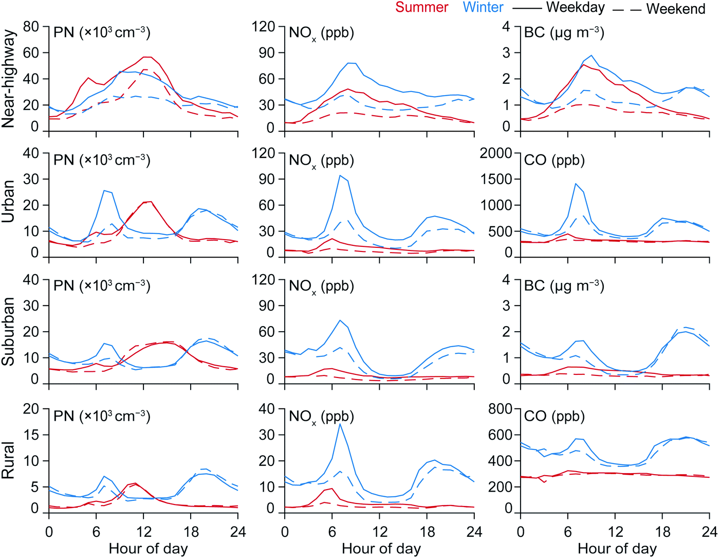 | ||
| Fig. 1 Average diurnal variations of PN and NOx for near-highway, urban, suburban, and rural sites by season (summer and winter). Separated by weekday and weekend to illustrate role of changing traffic volumes. We also include another primary pollutant (BC or CO depending on availability) for each site. All available hourly data of TRAP concentrations from Jul-2011 to Jan-2018 was used for these calculations. | ||
Average diurnal profiles indicate the combined influence of the traffic activity and ventilation patterns. In the winter, all sites showed a strong peak for all pollutants (PN, NOx, BC, and CO) during morning and evening rush hours, with concentrations 2–7× greater than the mid-day trough in concentrations (Fig. 1). In the ESI (Fig. S1†) we present the diurnal and seasonal averages for the ventilation coefficient (and other meteorological parameters) in the SF Bay Area. The lower wind speeds and mixing height during mornings and evenings of winter months resulted in lower ventilation. Conversely, owing to higher wind speeds and mixing height, warmer periods were generally more ventilated with the summer mid-days having the highest ventilation coefficient. Furthermore, some of the highest solar radiation was also observed during the summer daytime. The midday trough observed in all diurnal pollution profiles except those of summertime PN reflects the strong effect of increased atmospheric dilution during the middle of the day coupled with a reduction in traffic volumes on many urban roads outside of rush hour. Substantial weekday-weekend differences in these peaks demonstrate their dependence on weekday traffic. Winter NOx concentrations generally exceeded summer concentrations by 80–300%, reflecting increased dilution in summer months coupled with potential reduction in combustion sources. Rush hour concentrations were greatly reduced in summer months, especially during early evening hours, possibly because the higher boundary layer during the summer evenings caused greater mixing and dilution of traffic emissions, while winter commutes often take place when the boundary layer height is shallower.
Summertime PN patterns significantly diverged from those of other TRAPs. Unlike in winter conditions where NOx and PN peaks aligned during both mornings and evenings, summer patterns at all sites showed a mid-day PN peak that does not correspond to a peak in any other TRAP. This increase in PN without concomitant increases in other products of primary combustion, occurring during high-insolation midday hours (10 am to noon) and independent of weekend/weekday traffic differences, strongly suggests new particle formation (NPF). The summer daytime peak PN concentrations for non-near-highway sites were ∼3× greater than the concentrations observed during the rest of the day. At the near-highway site, high midday concentrations resulted in high concentrations throughout the day, without distinct peaks corresponding to morning and evening traffic-related sources. For winters, all sites except the near-highway site had early morning (∼6 am) and evening peaks (∼6 pm) for all pollutants (PN, NOx, BC, and CO). For example, the winter weekday morning PN concentration peaks were 1.4–1.6× higher higher than the midday troughs. For these non-nearhighway sites, morning PN peaks were 1.5–2.0× higher on weekdays than on weekends on average; evening winter peaks differed only slightly between weekdays and weekends (within 10%).
To highlight the diverging temporal patterns of PN and NOx, we computed the PN/NOx ratio. If a common primary source drives the concentrations of both PN and NOx in the urban environment, and both species have approximately similar lifetimes, then we would not expect the PN/NOx ratio to have strong time-dependence. Were these conditions met, NOx could serve as a proxy for PN. However, contrary to that assumption, we show that there is a strong mid-day enhancement in PN to NOx. In Fig. 2 we present the fixed-site diurnal variation in the PN/NOx ratio for winter and summer, and also separated by weekday-weekend. For all fixed sites, the PN/NOx ratio is highest during the summer daytime. Depending on time of day, the PN/NOx ratio for the near-highway site was 1–3× higher for summer than for winter. The largest difference between winter and summer PN/NOx ratio was observed for the urban and the suburban site with PN/NOx ratio between seasons ranging from 1–5× for urban and 1–5× for suburban. For the rural site the PN/NOx ratio was 1–4× higher during the summer compared to winter. Furthermore, summer PN/NOx were markedly higher on weekends which is consistent with the assumption that reduced weekend traffic results in lower concentrations of both NOx and associated directly-emitted PN, further accentuating the relative contribution of PN associated with NPF. It was notable that the absolute increase in the average weekend daytime PN peak concentrations from winter to summer was the highest for the near-highway site (+29900 cm−3) as compared to the urban (+13800 cm−3), suburban (+9400 cm−3), and the rural (+3000 cm−3) sites. The larger change in the absolute PN concentrations for more urban and generally polluted sites could be indicative of the role of locally-emitted semivolatile and intermediate precursors as contributors to daytime PN peaks during the summer months.72–74
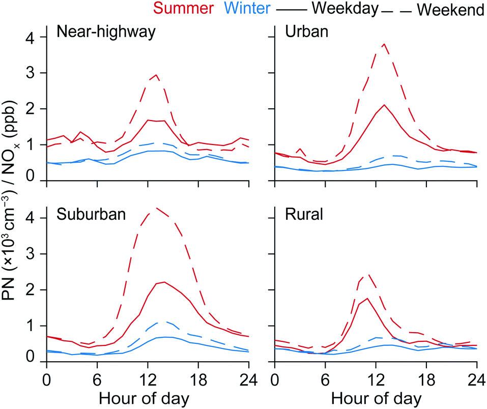 | ||
| Fig. 2 Average diurnal variations for PN/NOx ratio for near-highway, urban, suburban, and rural sites by season (summer and winter). Separated by weekday and weekend to illustrate role of changing traffic volumes. The values presented are the ratio of the averages, and not the average of the ratios. All available hourly data of TRAP concentrations from Jul-2011 to Jan-2018 was used for these calculations. | ||
We present in Table 1 the Spearman correlation (rs) matrix among the TRAPs for the near-highway, urban, suburban, and the rural sites based on hourly-average concentrations. At all sites, the correlation between PN and any other TRAP was 0.41–0.76. The inter-pollutant correlation among non-PN pollutants were generally higher compared to PN. NOx and BC were highly correlated at the near-highway site (rs = 0.91) and at the suburban site (rs = 0.91). NOx and CO were well correlated at the near-highway site (rs = 0.70) and the urban (rs = 0.81) site. Furthermore, for all the sites, PN concentrations were similarly correlated with NOx (rs,near-highway = 0.72, rs,urban = 0.66, rs,suburban = 0.49, rs, rural = 0.69) than either NO (0.76, 0.59, 0.44, 0.56) or NO2 (0.57, 0.66, 0.52, 0.68). For the suburban and rural sites, among the NOx species, NO was least correlated with PN and NO2 and NOx were similarly correlated to PN. The lifetime of NOx exceeds of that of NO and NO2: oxidation of NO to NO2 is one of the most rapid daytime NO sinks, and that photolysis of NO2 to NO is a rapid sink daytime sink of NO2. While interconversion of NO and NO2 occur at the timescales of a few minutes, NOx has a photochemical lifetime of 2–4 h.75
| PN | NO | NO2 | NOx | BC | CO | |
|---|---|---|---|---|---|---|
| Near-highway | ||||||
| PN | 1.00 | 0.76 | 0.57 | 0.72 | 0.73 | 0.43 |
| NO | 1.00 | 0.68 | 0.91 | 0.86 | 0.58 | |
| NO2 | 1.00 | 0.92 | 0.81 | 0.71 | ||
| NOx | 1.00 | 0.91 | 0.70 | |||
| BC | 1.00 | 0.67 | ||||
| CO | 1.00 | |||||
|
||||||
| Urban | ||||||
| PN | 1.00 | 0.59 | 0.66 | 0.66 | — | 0.54 |
| NO | 1.00 | 0.72 | 0.85 | — | 0.68 | |
| NO2 | 1.00 | 0.97 | — | 0.78 | ||
| NOx | 1.00 | — | 0.81 | |||
| BC | 1.00 | — | ||||
| CO | 1.00 | |||||
|
||||||
| Suburban | ||||||
| PN | 1.00 | 0.44 | 0.52 | 0.49 | 0.56 | — |
| NO | 1.00 | 0.68 | 0.77 | 0.70 | — | |
| NO2 | 1.00 | 0.98 | 0.90 | — | ||
| NOx | 1.00 | 0.91 | — | |||
| BC | 1.00 | — | ||||
| CO | 1.00 | |||||
|
||||||
| Rural | ||||||
| PN | 1.00 | 0.56 | 0.68 | 0.69 | — | 0.41 |
| NO | 1.00 | 0.70 | 0.83 | — | 0.46 | |
| NO2 | 1.00 | 0.97 | — | 0.54 | ||
| NOx | 1.00 | — | 0.55 | |||
| BC | 1.00 | — | ||||
| CO | 1.00 | |||||
To illuminate whether the low overall hourly correlation of PN and NOx was driven by seasonal factors, we performed an additional set of correlation analyses of hourly data stratified by season (Table 2). Lower pairwise correlation between PN and other TRAPs was driven by differences in summertime patterns – PN and NOx were least correlated during the summer daytime. For the non-near-highway sites, the summer daytime rs values were 0.01–0.53, suggesting that particularly during periods of higher photochemical activity, the dominant influence on NOx concentrations (traffic and other fuel combustion) differed from the dominant influence on PN concentrations (new particle formation from nucleation) during this period which had higher photochemical activity. The linear fit of weekly averaged NOx and the ventilation coefficient was higher than PN and the ventilation coefficient for all sites (ESI Fig. S4†). While the R2 values for NOx and the ventilation coefficient ranged between 0.19–0.51 across the fixed sites, the R2 between PN and the ventilation coefficient ranged between 0.00–0.34.
| Summer | Winter | All | |||||||
|---|---|---|---|---|---|---|---|---|---|
| Day | Night | All | Day | Night | All | Day | Night | All | |
| Near-highway | 0.59 | 0.84 | 0.79 | 0.79 | 0.64 | 0.70 | 0.66 | 0.72 | 0.72 |
| Urban | 0.53 | 0.77 | 0.59 | 0.73 | 0.74 | 0.73 | 0.57 | 0.81 | 0.66 |
| Suburban | 0.01 | 0.80 | 0.23 | 0.69 | 0.72 | 0.76 | 0.26 | 0.84 | 0.49 |
| Rural | 0.34 | 0.80 | 0.60 | 0.73 | 0.80 | 0.79 | 0.51 | 0.86 | 0.69 |
To further illustrate the dynamics of PN against other TRAPs at a higher temporal resolution, we developed a set of heatmaps representing the full timeseries of PN, NOx, and BC measurements with each day of the year (x-axis) divided into hourly concentrations (y-axis). Fig. 3 presents heatmaps for the suburban site, with the heatmaps for all sites presented in the ESI (Fig. S5–S8†). This visualization clearly illustrates how the diurnal profile of PN concentrations tracks the diurnal cycle of other traffic related air pollutants during winter months, and decouples from the TRAPs in other seasons. While the daytime PN concentration peaks are most apparent in the peak summer months (June–August), some daytime PN peaks can also be observed in April, May, and September. Based on this year-long heatmap, the months between October and March can be classified as the “low-NPF” season as compared to the summer which is the “high-NPF” season. To maximize the amount of mobile monitoring data that we can include for analysis (and thus improve our analytical precision and spatial coverage), we therefore use these low-NPF and high-NPF designations in our core analysis of mobile monitoring data. Sensitivity analyses presented in the ESI† demonstrate strong agreement in the spatial and temporal patterns of data between the low-NPF and winter periods, and between the high-NPF and summer periods (Fig. S9–S12†).
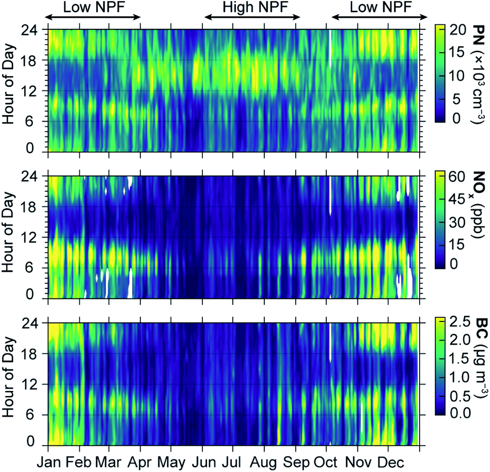 | ||
| Fig. 3 PN, NOx, and BC year-long concentrations shown as heatmap. While NOx and BC concentrations dropped throughout the day during the warmer periods, PN concentration during daytime of warmer months were similar to the morning and evening peaks observed during cooler periods. Based on data availability, we chose the data from the suburban site in 2015 (highest data coverage) for this heatmap. The colormap for each pollutant range from 0 to the 95th percentile of the hourly concentrations of that pollutant for the year and site presented. | ||
3.2 Spatiotemporal variation of PN and NOx: spatial patterns vary by season
In Fig. 4 we present the road-segment daytime mean concentrations of PN and NOx estimated on the basis of mobile monitoring in West Oakland and Downtown Oakland. Consistent with fixed-site measurements, these maps show the opposing seasonal patterns for PN and NOx. The on-road measurements were mostly made during the daytime making them more sensitive to photochemically-driven NPF. While on-road concentrations of PN increased from the low-NPF winter months to the high-NPF season, on-road concentrations of NOx decreased from the low-NPF to high-NPF conditions. Average on-road NOx levels decreased by a similar proportion for all road types: 29% for residential roads, 27% for arterials, and 27% for highways. This distributed decrease in NOx concentrations is consistent with the higher ventilation during the high-NPF season (summer). However, PN concentrations increased from low to high-NPF season for all road types. The increase in median PN levels from low- to high-NPF season was relatively lower for highways (+8900 cm−3, +24%), compared to the dramatic increase observed on arterials (+16000 cm−3, +64%), as well as residential roads (+18800 cm−3, +84%). While the spatial variation in NOx remained consistent between seasons, we see a decrease in the spatial variability of PN. As shown in Table 3, during the high-NPF season the interquartile range of concentrations on each road type was smaller than during the low-NPF season. We did not find evidence of such a trend for NOx. This relatively spatially uniform increase in PN levels during the high-NPF season suggests a potentially large contribution of nucleation to PN concentrations even for on-road concentrations during periods with high insolation.
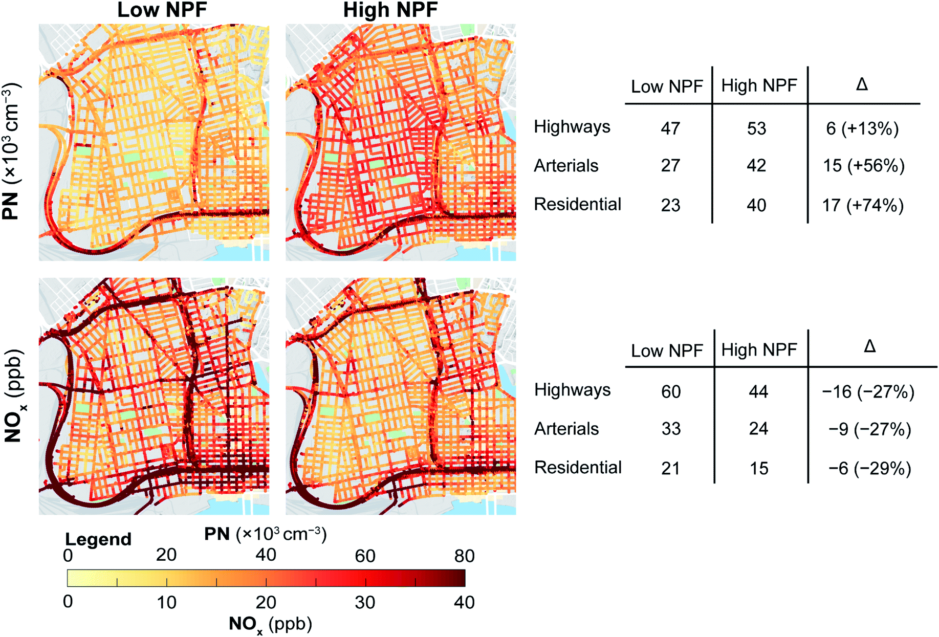 | ||
| Fig. 4 Median of drive pass mean of PN and NOx for low-NPF and high-NPF seasons. Average (mean) concentrations by road type and change from low-NPF to high-NPF seasons are also tabulated. Mobile monitoring measurements were made during the daytime in West Oakland and Downtown Oakland (May-2015–May-2017). | ||
| Pollutant | Road type | Mean | 25th percentile | Median | 75th percentile | ||||
|---|---|---|---|---|---|---|---|---|---|
| L-NPF | H-NPF | L-NPF | H-NPF | L-NPF | H-NPF | L-NPF | H-NPF | ||
| PN (103 cm−3) | Highway | 47.3 | 52.5 | 28.9 | 33.5 | 36.7 | 45.6 | 56.6 | 63.8 |
| Arterial | 26.9 | 41.8 | 21.3 | 34.2 | 25.1 | 41.1 | 30.4 | 48.5 | |
| Residential | 23.2 | 40.4 | 18.8 | 32.8 | 22.3 | 41.1 | 26.2 | 47.4 | |
| NOx (ppb) | Highway | 59.8 | 43.8 | 36.9 | 25.0 | 50.2 | 35.3 | 76.0 | 53.5 |
| Arterial | 33.4 | 24.3 | 21.6 | 15.8 | 28.0 | 20.3 | 40.1 | 27.7 | |
| Residential | 20.8 | 15.5 | 14.7 | 12.2 | 18.4 | 14.1 | 24.4 | 17.2 | |
We show maps of the PN/NOx ratio to indicate road-types and times when the PN levels deviated sharply from NOx. To make our analysis less sensitive to outliers in instantaneous PN and NOx mobile measurements, we computed the ratio of the road-segment median concentrations. In Fig. 5 we present the spatiotemporal and seasonal variation in the PN/NOx ratio. In general, the PN/NOx ratio for on-road concentrations was higher for the high-NPF season daytime compared to the low-NPF season. The seasonal difference was the highest for residential roads with 1–4 pm PN/NOx ratio ∼6× higher for the high-NPF season compared to the low-NPF season. For the arterial roads, the high-NPF season PN/NOx ratio was ∼4× higher than low-NPF season between 12–5 pm. The seasonal difference in the high-NPF season and low-NPF season PN/NOx ratio was the least for the highways (∼2× higher than low-NPF season between 11 am–5 pm). The PN/NOx ratio was highest for residential streets since they have the lowest NOx concentrations and the PN concentrations would be less spatially variable during NPF events (a regional phenomenon). Overall, the diurnal profiles of the PN/NOx ratio from on-road measurements corroborate the findings from the fixed sites (Fig. 2), and emphasize how the seasonal divergence in this ratio is most strongly observed in locales that are relatively less influenced by direct traffic emissions. As with fixed site hourly data, time-averaged road segment concentrations show lower correlation summertime on all road types during the summer (Table S4†), with a particularly notable decrease on residential roads.
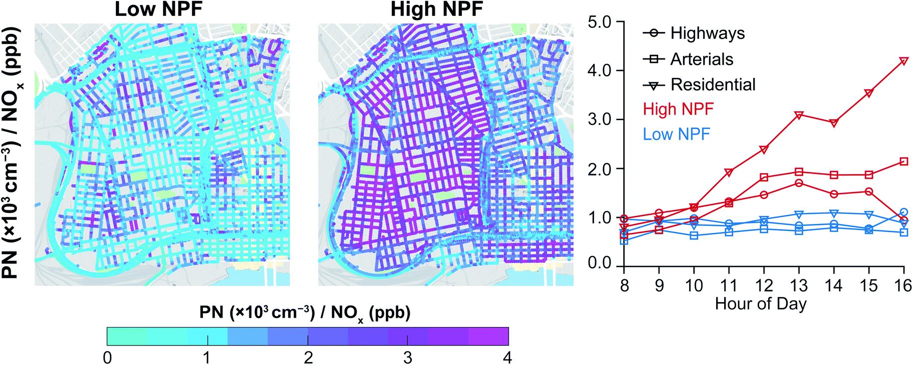 | ||
| Fig. 5 Spatial map of PN/NOx ratio for low-NPF and high-NPF seasons. The diurnal variation of PN/NOx ratio by road type are also presented. The values presented are the ratio of the averages, and not the average of the ratios. Mobile monitoring measurements were made during the daytime in West Oakland and Downtown Oakland (May-2015–May-2017). | ||
4 Conclusions
UFP levels are governed by an interplay between proximity to sources such as traffic, diurnal and seasonal ventilation changes, and new particle formation from nucleation. By using long term measurements from fixed-sites and highly spatially resolved on-road data, we were able to analyze spatiotemporal variation of PN concentrations. We observed daytime peaks in PN concentrations at multiple sites during the warmer months that were not observed for other primary traffic-related pollutants. In approximate terms, we observed a ∼2× increase of PN concentrations during mid-day hours relative to the morning rush hours, while NOx and other TRAP pollutant concentrations typically dropped by ∼2× over the same period. We take this finding as further evidence that NPF can complement traffic as a major source of ambient PN. In very rough terms, this finding implies that for the half of the year where NPF is common in the SF Bay Area, approximately half or more of the PN concentrations might be attributed to new particle formation during the peak hours for this photochemical process. Because the spatiotemporal variation in NOx concentrations differs from PN, using NOx (or other traffic-related air pollutants) as a proxy for PN (or UFP) concentrations could result in inaccuracies in estimating UFP exposure. These findings may have particular relevance for high insolation urban areas where NPF can contribute to a large fraction of UFP concentrations.21 It should also be noted that while PN concentrations are generally a good proxy for UFP concentrations in urban ambient air in the USA, this assumption does not hold for extremely polluted environments where a large fraction of the particles can be larger than 100 nm.44,76Long-term fixed site and mobile monitoring measurements can advance understanding of the spatiotemporal patterns of various air pollutants.65,77 While highly resolved spatio-temporal measurements of particle size distributions may be unlikely, a compromise such as the collection of long term measurements of size distributions along a gradient of fixed site locations may help us understand the role of primary emissions vs. NPF in contributing to UFP concentrations. Furthermore, recent advances in understanding semivolatile and intermediate volatility precursors, and the emerging recognition of the pivotal role of volatile chemical emissions72 in urban reactive chemistry might suggest that this issue merits detailed investigation from a chemically resolved perspective as well.
Our findings should inform future assessment modeling of urban UFP exposure: while traffic activity and the location of major roadways are governing factors in temporal and spatial patterns of TRAP concentrations (including UFP), the effect of NPF during sunny/warmer seasons substantially alters both temporal and spatial UFP trends. The decoupling of trends between UFP and other TRAPs could result in inaccuracies in exposure modeling. First, if the model assumes or implies a fixed ratio between UFP and other TRAPs (i.e., PN/NOx ratio) based on a single season of sampling, it may significantly misrepresent UFP patterns. The ratio is highly seasonally dependent, as well as dependent on time-of-day. Second, if the model overweights the importance of roadway proximity or traffic activity, the exposure in residential or far-from-road areas would be substantially underestimated for summer months. Activity-based exposure models, which integrate exposure over a range of locations reflecting an individual's daily activities, would be particularly impacted by assuming NOx is an appropriate surrogate for UFP. For example, higher UFP concentrations during the daytime can imply higher exposure during this time when people are more likely to be outdoors. NPF can contribute to substantial UFP concentrations and the contribution can be higher for locations with higher concentrations of UFP precursors. There is growing evidence of the adverse health effects of UFP. A final public health implication of these findings is that reductions in exposure to UFP cannot rely only on reducing direct emissions, they must also depend on the reduction of UFP precursors.
Author contributions
Conceptualization: SG, SEC, and JSA; data curation: SG, SEC, and KPM; formal analysis: SG and SEC; funding acquisition: JSA; methodology: all authors; visualization: SG and SEC; writing – original draft: SG and SEC; writing – review & editing: all authors.Conflicts of interest
There are no conflicts to declare. ML is employed by Aclima, Inc. Research described in this article was funded by the Health Effects Institute, an organization jointly funded by the United States Environmental Protection Agency (assistance award no. R-82811201) and certain motor vehicle and engine manufacturers. The contents of this article do not necessarily reflect the views of Health Effects Institute, or its sponsors, nor do they necessarily reflect the views and policies of the United States Environmental Protection Agency or motor vehicle and engine manufacturers.Acknowledgements
The authors would like to acknowledge support from the Bay Area Air Quality Management District (especially, David Holstius and Philip Martien), Aclima Inc. (especially, Okorie Puryear, Brian LaFranchi, and the Aclima mobile platform team), Google (especially, Carol Owens, Karin Tuxen-Bettman, and the Google Street View team and drivers), Lawrence Berkeley National Laboratory (especially, Thomas Kirchstetter), and the Department of Civil, Architectural and Environmental Engineering at the University of Texas at Austin (especially, Kerry Kinney, Paola Passalacqua, and Lea Hildebrandt Ruiz). This work was funded by the Environmental Defense Fund and the Health Effects Institute.References
- D. E. Schraufnagel, J. R. Balmes, C. T. Cowl, S. D. Matteis, S.-H. Jung, K. Mortimer, R. Perez-Padilla, M. B. Rice, H. Riojas-Rodriguez, A. Sood, G. D. Thurston, T. To, A. Vanker and D. J. Wuebbles, Chest, 2019, 155, 409–416 CrossRef PubMed.
- D. E. Schraufnagel, J. R. Balmes, C. T. Cowl, S. D. Matteis, S.-H. Jung, K. Mortimer, R. Perez-Padilla, M. B. Rice, H. Riojas-Rodriguez, A. Sood, G. D. Thurston, T. To, A. Vanker and D. J. Wuebbles, Chest, 2019, 155, 417–426 CrossRef PubMed.
- G. Oberdörster, E. Oberdörster and J. Oberdörster, Environ. Health Perspect., 2005, 113, 823–839 CrossRef PubMed.
- I. Salma, P. Füri, Z. Németh, I. Balásházy, W. Hofmann and Á. Farkas, Atmos. Environ., 2015, 104, 39–49 CrossRef CAS.
- S. Weichenthal, T. Olaniyan, T. Christidis, E. Lavigne, M. Hatzopoulou, K. Van Ryswyk, M. Tjepkema and R. Burnett, Epidemiology, 2020, 31, 177–183 CrossRef PubMed.
- B. A. Maher, I. A. M. Ahmed, V. Karloukovski, D. A. MacLaren, P. G. Foulds, D. Allsop, D. M. A. Mann, R. Torres-Jardón and L. Calderon-Garciduenas, Proc. Natl. Acad. Sci., 2016, 113, 10797–10801 CrossRef CAS PubMed.
- G. Oberdörster, Z. Sharp, V. Atudorei, A. Elder, R. Gelein, W. Kreyling and C. Cox, Inhalation Toxicol., 2004, 16, 437–445 CrossRef PubMed.
- Health Effects Institute, Understanding the Health Effects of Ambient Ultrafine Particles, 2013, https://www.healtheffects.org/publication/understanding-health-effects-ambient-ultrafine-particles Search PubMed.
- N. Li, C. Sioutas, A. Cho, D. Schmitz, C. Misra, J. Sempf, M. Wang, T. Oberley, J. Froines and A. Nel, Environ. Health Perspect., 2003, 111, 455–460 CrossRef CAS PubMed.
- T. Xia, P. Korge, J. N. Weiss, N. Li, M. I. Venkatesen, C. Sioutas and A. Nel, Environ. Health Perspect., 2004, 112, 1347–1358 CrossRef CAS PubMed.
- A. Nel, Science, 2005, 308, 804–806 CrossRef CAS PubMed.
- R. W. Atkinson, G. W. Fuller, H. R. Anderson, R. M. Harrison and B. Armstrong, Epidemiology, 2010, 21, 501–511 CrossRef PubMed.
- R. Li, D. Mittelstein, W. Kam, P. Pakbin, Y. Du, Y. Tintut, M. Navab, C. Sioutas and T. Hsiai, Am. J. Physiol.: Cell Physiol., 2013, 304, C362–C369 CrossRef CAS PubMed.
- S. Ohlwein, R. Kappeler, M. Kutlar Joss, N. Künzli and B. Hoffmann, Int. J. Public Health, 2019, 64, 547–559 CrossRef PubMed.
- L. Järvi, H. Hannuniemi, T. Hussein, H. Junninen, P. Aalto, P. Keronen, M. Kulmala, P. P Keronen, R. Hillamo, T. Mäkelä, E. Siivola and T. Vesala, Boreal Environ. Res., 2009, 14, 1797–2469 Search PubMed.
- K. Moore, M. Krudysz, P. Pakbin, N. Hudda and C. Sioutas, Aerosol Sci. Technol., 2009, 43, 587–603 CrossRef CAS.
- W. Birmili, K. Weinhold, F. Rasch, A. Sonntag, J. Sun, M. Merkel, A. Wiedensohler, S. Bastian, A. Schladitz, G. Löschau, J. Cyrys, M. Pitz, J. Gu, T. Kusch, H. Flentje, U. Quass, H. Kaminski, T. A. J. Kuhlbusch, F. Meinhardt, A. Schwerin, O. Bath, L. Ries, H. Gerwig, K. Wirtz and M. Fiebig, Earth System Science Data, 2016, 8, 355–382 CrossRef.
- R. C. Abernethy, R. W. Allen, I. G. McKendry and M. Brauer, Environ. Sci. Technol., 2013, 47, 5217–5225 CrossRef CAS PubMed.
- G. Hoek, Curr. Environ. Health Rep., 2017, 4, 450–462 CrossRef CAS PubMed.
- M. Brines, M. Dall'Osto, D. Beddows, R. M. Harrison and X. Querol, Atmos. Chem. Phys., 2014, 14, 2973–2986 CrossRef CAS.
- M. Brines, M. Dall'Osto, D. C. S. Beddows, R. M. Harrison, F. Gómez-Moreno, L. Núñez, B. Artíñano, F. Costabile, G. P. Gobbi, F. Salimi, L. Morawska, C. Sioutas and X. Querol, Atmos. Chem. Phys., 2015, 15, 5929–5945 CrossRef CAS.
- H. Z. Li, P. Gu, Q. Ye, N. Zimmerman, E. S. Robinson, R. Subramanian, J. S. Apte, A. L. Robinson and A. A. Presto, Atmos. Environ.: X, 2019, 2, 100012 CAS.
- R. M. Harrison, A. M. Jones, J. Gietl, J. Yin and D. C. Green, Environ. Sci. Technol., 2012, 46, 6523–6529 CrossRef CAS PubMed.
- G. Cohen, D. Steinberg, Yuval, I. Levy, S. Chen, J. Kark, N. Levin, G. Witberg, T. Bental, D. Broday, R. Kornowski and Y. Gerber, Environ. Res., 2019, 108560 CrossRef CAS PubMed.
- J. D. Kaufman, S. D. Adar, R. G. Barr, M. Budoff, G. L. Burke, C. L. Curl, M. L. Daviglus, A. V. D. Roux, A. J. Gassett, D. R. Jacobs, R. Kronmal, T. V. Larson, A. Navas-Acien, C. Olives, P. D. Sampson, L. Sheppard, D. S. Siscovick, J. H. Stein, A. A. Szpiro and K. E. Watson, Lancet, 2016, 388, 696–704 CrossRef CAS.
- I. Levy, C. Mihele, G. Lu, J. Narayan and J. R. Brook, Environ. Health Perspect., 2014, 122, 65–72 CrossRef PubMed.
- R. McConnell, T. Islam, K. Shankardass, M. Jerrett, F. Lurmann, F. Gilliland, J. Gauderman, E. Avol, N. Künzli, L. Yao, J. Peters and K. Berhane, Environ. Health Perspect., 2010, 118, 1021–1026 CrossRef CAS PubMed.
- W. James Gauderman, E. Avol, F. Lurmann, N. Kuenzli, F. Gilliland, J. Peters and R. McConnell, Epidemiology, 2005, 16, 737–743 CrossRef PubMed.
- M. Jerrett, K. Shankardass, K. Berhane, W. James Gauderman, N. Kuenzli, E. Avol, F. Gilliland, F. Lurmann, J. N. Molitor, J. T Molitor, D. Thomas, J. Peters and R. McConnell, Environ. Health Perspect., 2008, 116, 1433–1438 CrossRef PubMed.
- A. P. Patton, J. Perkins, W. Zamore, J. I. Levy, D. Brugge and J. L. Durant, Atmos. Environ., 2014, 99, 309–321 CrossRef CAS PubMed.
- G. Hagler, R. Baldauf, E. Thoma, T. Long, R. Snow, J. Kinsey, L. Oudejans and B. Gullett, Atmos. Environ., 2009, 43, 1229–1234 CrossRef CAS.
- B. Beckerman, M. Jerrett, J. R. Brook, D. K. Verma, M. A. Arain and M. M. Finkelstein, Atmos. Environ., 2008, 42, 275–290 CrossRef CAS.
- I. Longley, D. Inglis, M. Gallagher, P. Williams, J. Allan and H. Coe, Atmos. Environ., 2005, 39, 5157–5169 CrossRef CAS.
- M. Ketzel, P. Wåhlin, R. Berkowicz and F. Palmgren, Atmos. Environ., 2003, 37, 2735–2749 CrossRef CAS.
- H. Boogaard, G. P. Kos, E. P. Weijers, N. A. Janssen, P. H. Fischer, S. C. van der Zee, J. J. de Hartog and G. Hoek, Atmos. Environ., 2011, 45, 650–658 CrossRef CAS.
- P. M. Fine, S. Shen and C. Sioutas, Aerosol Sci. Technol., 2004, 38, 182–195 CrossRef CAS.
- F. Costabile, W. Birmili, S. Klose, T. Tuch, B. Wehner, A. Wiedensohler, U. Franck, K. König and A. Sonntag, Atmos. Chem. Phys., 2009, 9, 3163–3195 CrossRef CAS.
- M. Kulmala, H. Vehkamäki, T. Petäjä, M. D. Maso, A. Lauri, V.-M. Kerminen, W. Birmili and P. McMurry, J. Aerosol Sci., 2004, 35, 143–176 CrossRef CAS.
- M. Boy and M. Kulmala, Atmos. Chem. Phys., 2002, 2, 1–16 CrossRef CAS.
- M. Kulmala, T. Suni, K. E. J. Lehtinen, M. Dal Maso, M. Boy, A. Reissell, U. Rannik, P. Aalto, P. Keronen, H. Hakola, J. Bäck, T. Hoffmann, T. Vesala and P. Hari, Atmos. Chem. Phys., 2004, 4, 557–562 CrossRef CAS.
- C. O’Dowd, C. Monahan and M. Dall’Osto, Geophys. Res. Lett., 2010, 37, L19805 Search PubMed.
- K. Sellegri, P. Laj, H. Venzac, J. Boulon, D. Picard, P. Villani, P. Bonasoni, A. Marinoni, P. Cristofanelli and E. Vuillermoz, Atmos. Chem. Phys., 2010, 10, 10679–10690 CrossRef CAS.
- V. Vakkari, H. Laakso, M. Kulmala, A. Laaksonen, D. Mabaso, M. Molefe, N. Kgabi and L. Laakso, Atmos. Chem. Phys., 2011, 11, 3333–3346 CrossRef CAS.
- S. Gani, S. Bhandari, K. Patel, S. Seraj, P. Soni, Z. Arub, G. Habib, L. Hildebrandt Ruiz and J. S. Apte, Atmos. Chem. Phys., 2020, 20, 8533–8549 CrossRef CAS.
- K. S. Woo, D. R. Chen, D. Y. H. Pui and P. H. McMurry, Aerosol Sci. Technol., 2001, 34, 75–87 CrossRef CAS.
- L.-H. Young and G. J. Keeler, J. Air Waste Manage. Assoc., 2004, 54, 1079–1090 CrossRef PubMed.
- C.-H. Jeong, G. J. Evans, P. K. Hopke, D. J. Chalupa and M. Utell, J. Air Waste Manage. Assoc., 2006, 56, 431–443 CrossRef CAS PubMed.
- Z. Wu, M. Hu, P. Lin, S. Liu, B. Wehner and A. Wiedensohler, Atmos. Environ., 2008, 42, 7967–7980 CrossRef CAS.
- X. J. Shen, J. Y. Sun, Y. M. Zhang, B. Wehner, A. Nowak, T. Tuch, X. C. Zhang, T. T. Wang, H. G. Zhou, X. L. Zhang, F. Dong, W. Birmili and A. Wiedensohler, Atmos. Chem. Phys., 2011, 11, 1565–1580 CrossRef CAS.
- I. Salma, T. Borsós, T. Weidinger, P. Aalto, T. Hussein, M. Dal Maso and M. Kulmala, Atmos. Chem. Phys., 2011, 11, 1339–1353 CrossRef CAS.
- D. Řimnáčová, V. Ždímal, J. Schwarz, J. Smolík and M. Řimnáč, Atmos. Res., 2011, 101, 539–552 CrossRef.
- R. Betha, D. V. Spracklen and R. Balasubramanian, Atmos. Environ., 2013, 71, 340–351 CrossRef CAS.
- N. Hudda, K. Cheung, K. F. Moore and C. Sioutas, Atmos. Chem. Phys., 2010, 10, 11385–11399 CrossRef CAS.
- S. Hama, R. Cordell and P. Monks, Atmos. Environ., 2017, 166, 62–78 CrossRef CAS.
- Q. Zhang, C. O. Stanier, M. R. Canagaratna, J. T. Jayne, D. R. Worsnop, S. N. Pandis and J. L. Jimenez, Environ. Sci. Technol., 2004, 38, 4797–4809 CrossRef CAS PubMed.
- Z. Ning, M. D. Geller, K. F. Moore, R. Sheesley, J. J. Schauer and C. Sioutas, Environ. Sci. Technol., 2007, 41, 6000–6006 CrossRef CAS PubMed.
- J. Pey, S. Rodřguez, X. Querol, A. Alastuey, T. Moreno, J. P. Putaud and R. van Dingenen, Atmos. Environ., 2008, 42, 9052–9062 CrossRef CAS.
- H. C. Cheung, C. C.-K. Chou, W.-R. Huang and C.-Y. Tsai, Atmos. Chem. Phys., 2013, 13, 8935–8946 CrossRef.
- D. Westerdahl, S. Fruin, T. Sax, P. M. Fine and C. Sioutas, Atmos. Environ., 2005, 39, 3597–3610 CrossRef CAS.
- G. S. Hagler, E. D. Thoma and R. W. Baldauf, J. Air Waste Manage. Assoc., 2010, 60, 328–336 CrossRef CAS PubMed.
- J. Peters, J. Theunis, M. Van Poppel and P. Berghmans, Aerosol Air Qual. Res., 2013, 13, 509–522 CrossRef.
- S. Hankey and J. D. Marshall, Atmos. Environ., 2015, 122, 65–73 CrossRef CAS.
- M. C. Simon, N. Hudda, E. N. Naumova, J. I. Levy, D. Brugge and J. L. Durant, Atmos. Environ., 2017, 169, 113–127 CrossRef CAS PubMed.
- Bay Area Air Quality Management District, Ambient Air Monitoring Network, 2019, http://www.baaqmd.gov/about-air-quality/air-quality-measurement/ambient-air-monitoring-network Search PubMed.
- J. S. Apte, K. P. Messier, S. Gani, M. Brauer, T. W. Kirchstetter, M. M. Lunden, J. D. Marshall, C. J. Portier, R. C. Vermeulen and S. P. Hamburg, Environ. Sci. Technol., 2017, 51, 6999–7008 CrossRef CAS PubMed.
- K. P. Messier, S. E. Chambliss, S. Gani, R. Alvarez, M. Brauer, J. J. Choi, S. P. Hamburg, J. Kerckhoffs, B. LaFranchi, M. M. Lunden, J. D. Marshall, C. J. Portier, A. Roy, A. A. Szpiro, R. C. H. Vermeulen and J. S. Apte, Environ. Sci. Technol., 2018, 52, 12563–12572 CrossRef CAS PubMed.
- S. Hu, S. Fruin, K. Kozawa, S. Mara, S. E. Paulson and A. M. Winer, Atmos. Environ., 2009, 43, 2541–2549 CrossRef CAS PubMed.
- R. Gelaro, W. McCarty, M. J. Suárez, R. Todling, A. Molod, L. Takacs, C. A. Randles, A. Darmenov, M. G. Bosilovich, R. Reichle, K. Wargan, L. Coy, R. Cullather, C. Draper, S. Akella, V. Buchard, A. Conaty, A. M. da Silva, W. Gu, G.-K. Kim, R. Koster, R. Lucchesi, D. Merkova, J. E. Nielsen, G. Partyka, S. Pawson, W. Putman, M. Rienecker, S. D. Schubert, M. Sienkiewicz and B. Zhao, J. Clim., 2017, 30, 5419–5454 CrossRef PubMed.
- California Department of Transportation, Freeway Performance Measurement System, 2019, http://pems.dot.ca.gov/ Search PubMed.
- P. K. Saha, N. Zimmerman, C. Malings, A. Hauryliuk, Z. Li, L. Snell, R. Subramanian, E. Lipsky, J. S. Apte, A. L. Robinson and A. A. Presto, Sci. Total Environ., 2019, 655, 473–481 CrossRef CAS PubMed.
- B. C. McDonald, D. R. Gentner, A. H. Goldstein and R. A. Harley, Environ. Sci. Technol., 2013, 47, 10022–10031 CrossRef CAS PubMed.
- B. C. McDonald, J. A. d. Gouw, J. B. Gilman, S. H. Jathar, A. Akherati, C. D. Cappa, J. L. Jimenez, J. Lee-Taylor, P. L. Hayes, S. A. McKeen, Y. Y. Cui, S.-W. Kim, D. R. Gentner, G. Isaacman-VanWertz, A. H. Goldstein, R. A. Harley, G. J. Frost, J. M. Roberts, T. B. Ryerson and M. Trainer, Science, 2018, 359, 760–764 CrossRef CAS PubMed.
- Y. Zhao, N. T. Nguyen, A. A. Presto, C. J. Hennigan, A. A. May and A. L. Robinson, Environ. Sci. Technol., 2016, 50, 4554–4563 CrossRef CAS PubMed.
- P. K. Saha, S. M. Reece and A. P. Grieshop, Environ. Sci. Technol., 2018, 52, 7192–7202 CrossRef CAS PubMed.
- S. Sillman, Atmos. Environ., 1999, 33, 1821–1845 CrossRef CAS.
- T. Wu and B. E. Boor, Atmos. Chem. Phys., 2021, 21, 8883–8914 CrossRef CAS.
- P. K. Saha, S. Sengupta, P. Adams, A. L. Robinson and A. A. Presto, Environ. Sci. Technol., 2020, 54, 9295–9304 CrossRef CAS PubMed.
Footnotes |
| † Electronic supplementary information (ESI) available. See DOI: 10.1039/d1ea00058f |
| ‡ These authors contributed equally to this work. |
| This journal is © The Royal Society of Chemistry 2021 |