DOI:
10.1039/D1EA00038A
(Critical Review)
Environ. Sci.: Atmos., 2021,
1, 297-345
Aging of atmospheric aerosols and the role of iron in catalyzing brown carbon formation†
Received
11th May 2021
, Accepted 6th July 2021
First published on 7th July 2021
Abstract
Extensive research has been done on the processes that lead to the formation of secondary organic aerosol (SOA) including the atmospheric oxidation of volatile organic compounds (VOCs) from biogenic and anthropogenic sources, gas–particle partitioning, and multiphase/heterogeneous reactions. Also, a number of chemical and photochemical aging processes of primary aerosols and SOA were reported to lead to the formation of “brown carbon (BrC)”, a term that refers to light absorbing soluble and insoluble components. However, the role of transition metals such as iron in these processes is not well understood. This review summarized the current state of knowledge on iron chemistry that lead to BrC formation. Dark iron chemistry with phenolic and aliphatic organic precursors is shown to be responsible for the efficient formation of soluble and insoluble BrC, including organonitrogen compounds, under a wide range of atmospheric aerosol physical states and chemical compositions. These efficient processes are not completely suppressed in the presence of competing ligands or light. The atmospheric impact of SOA and BrC from these pathways is discussed in the context of aerosols' direct and indirect effects on the climate. Additional laboratory, field, and modeling studies are needed to better understand the contributions of these potentially important metal-catalyzed pathways to SOA and BrC formation and the overall aerosol chemistry.
 Hind A. Al-Abadleh | Hind A. Al-Abadleh is a Full Professor in the Department of Chemistry and Biochemistry at Wilfrid Laurier University. She is the 2021–2022 University Research Professor, a Fellow at the Balsillie School of International Affairs in Waterloo, Ontario, Canada, and was the 2019 Fulbright Canada Visiting Research Chair in Atmospheric Chemistry, Air Quality, and Climate Change at the University of California Irvine. The active research programs in her lab are in the fields of atmospheric chemistry, air quality, geochemistry, and environmental remediation. Among her leadership roles, Al-Abadleh is the current Chair of the Environment Division of the Chemical Institute of Canada and Vice Chair of the Special Interest Group on Atmosphere-Related Research in Canadian Universities (ARRCU) at the Canadian Meteorological and Oceanographic Society (CMOS). |
Environmental significance
Atmospheric aerosols contribute to the climate radiative forcing through their aerosol–radiation and aerosol–cloud interactions. Particles that are darker in color are expected to have a stronger direct effect on the climate by absorbing solar radiation. Also, salts and mineral dust particles are efficient cloud and ice condensation nuclei. However, the extent of the above interactions remains highly uncertain stemming from the multitude of chemicals and processing pathways that modify aerosols' physicochemical properties. Dust particles from natural and human activities contain iron, which is the fourth most abundant element by mass in the Earth's crust. Through long range transport and atmospheric processing, these particles frequently mix with organic gases and particles such as those in biomass burning smoke. This review shows that iron is capable of catalyzing chemical reactions with organics that make aerosol particles more light-absorbing over a wide range of conditions. These new pathways are currently unaccounted for in atmospheric models and hence their inclusion would improve the parameterization of processes that lead to secondary organic aerosol formation and aging, and ultimately impacts on the climate.
|
1. Introduction
Atmospheric aerosol particles in the lower troposphere originate from primary sources and secondary processes.1–7 Aerosol particles from primary sources include mineral dust, sea spray, terrestrial primary biological aerosol particles (bioparticles for short) such as fungal spores and pollen, primary organic aerosol such as brown carbon (BrC) and black carbon (BC) from biomass burning events referred to as biomass burning organic aerosol (BBOA). Also, an emerging class of ‘unconventional’ mineral dust is the one produced from rapid urbanization and industrialization, particularly in developing countries. This class is referred to as anthropogenic fugitive, combustion, and industrial dust (AFCID),8 which largely contributes to fine particulate matter (PM2.5) known to be harmful to human health.9–11
Secondary processes refer to particle formation and growth from reactions in the atmosphere among inorganic and organic precursors in the gas and condensed phases. These reactions lead to the formation of ammonium, non-sea salt sulfates, nitrates, and secondary organic aerosol (SOA) particles,12–15 from ammonia, sulfur-containing gases such as sulfur oxides, nitrogen oxides, and volatile organic compounds (VOCs) of biogenic16 and anthropogenic17 origins. The organic component in the fine aerosol particle fraction (diameter less than 1 μm) contributes to more than 50% of the aerosol mass.15 Aerosol particle resident time ranges from hours up to 10–15 days during which they undergo long range transport over thousands of miles.18 They are removed from the atmosphere mainly via sedimentation and dry and wet deposition. As a result, atmospheric aerosol particles contribute to the biogeochemical cycles of nutrients such as nitrogen, phosphorus, iron and other transition metals.19–21
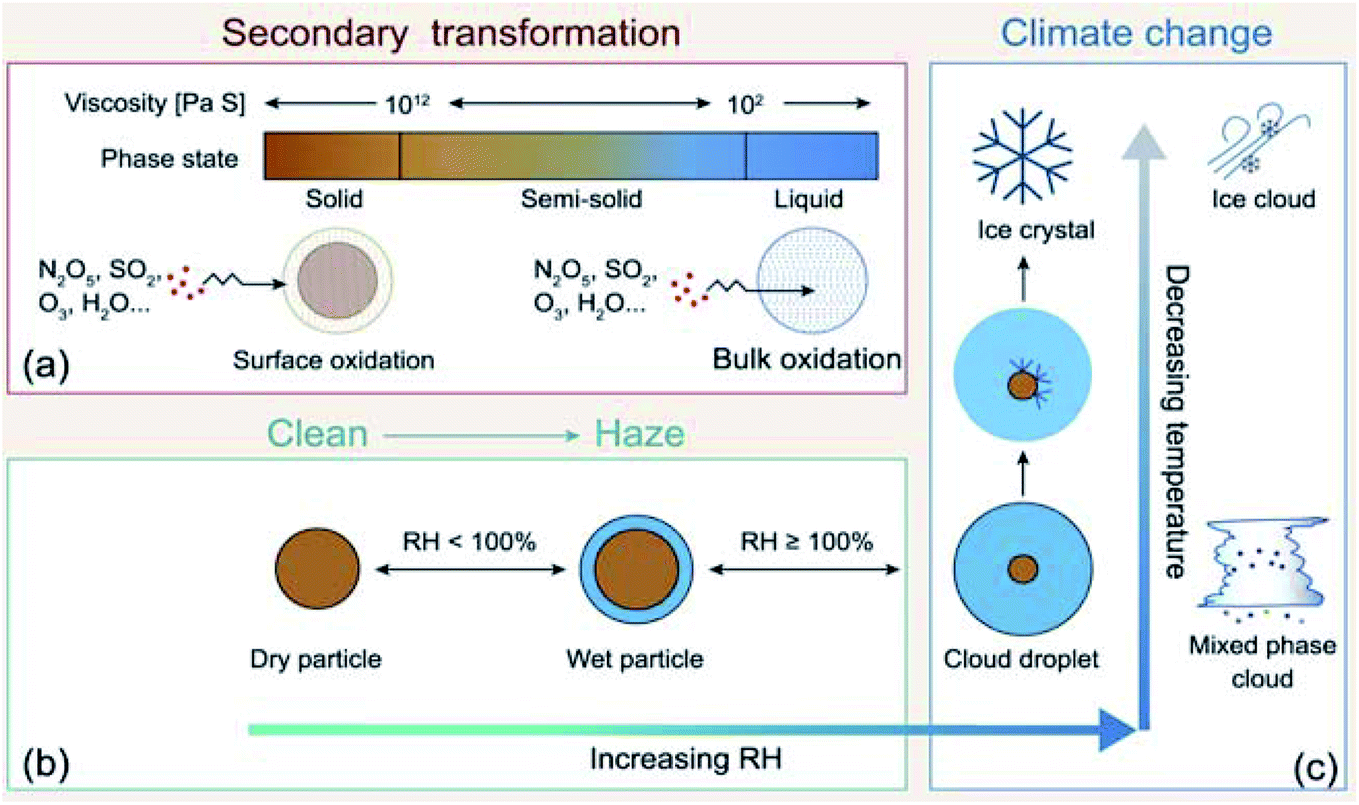
Atmospheric aerosol particles impact the climate system because they have complex physical and chemical properties that evolve over time and govern their lifetime in the atmosphere.22 These properties also govern their biological and toxicological impacts, which are of importance to understand and quantify the aerosol effects on ocean productivity and human health,23 respectively. McMurry published a review of atmospheric aerosol measurements of physical and chemical properties,24 which are classified into categories according to the instrumental capacity to resolve their size, time and composition. Since McMurry's paper, edited books25,26 and a number of reviews were published on advanced analytical tools27 used to study the hygroscopic properties and water uptake,28 ice nucleation,29,30 aerosol morphology and mixing states,31,32 optical properties,33 viscosity,34 liquid–liquid phase separation,35 acidity,36,37 and chemical composition.15,38–42
All of the aforementioned properties contribute to the direct and indirect effects of aerosol particles on the climate. The direct effect of aerosol particles refers to their role in modifying the planetary energy balance (i.e., radiative forcing) and precipitation, which has the highest uncertainty in climate and weather models.6 Aerosol particles affect the radiative forcing directly through absorption and scattering of shortwave and longwave radiation. This effect is quantified through the radiative forcing due to the aerosol–radiation interaction term (RFari) in W m−2. Positive RFari indicates heating effects and negative RFari indicates cooling. RFari values for different anthropogenic aerosol types are shown in Fig. 1, for the 1750–2010 period. Fig. 1 also shows that the highest uncertainty in RFari is associated with the organic content of atmospheric aerosol particles, with BC resulting in the net heating effect, and BBOA and SOA having both heating and cooling effects.
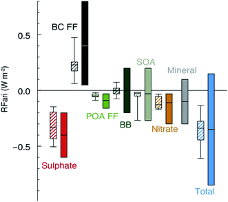 |
| | Fig. 1 Annual mean top of the atmosphere radiative forcing due to aerosol–radiation interactions (RFari, in W m−2) due to different anthropogenic aerosol types, for the 1750–2010 period. Hatched whisker boxes show median (line), 5th to 95th percentile ranges (box) and min/max values (whiskers) from AeroCom II models43 corrected for the 1750–2010 period. Solid coloured boxes show the IPCC Assessment Report 5 (AR5) best estimates and 90% uncertainty ranges. BC FF is for black carbon from the fossil fuel (FF) and the biofuel, POA FF is for primary organic aerosol from fossil fuel and biofuel, BB is short for BBOA for biomass burning organic aerosols and SOA is for secondary organic aerosol. The figure and the caption were reproduced from ref. 1 with permission from Cambridge University Press, © 2013. | |
The indirect effects of aerosols are related to cloud formation and lifetime and modification of atmospheric composition through multiphase and heterogeneous surface chemistry. Aerosol particle–cloud interactions are coupled by a multitude of dynamical and physical processes that span multitemporal and spatial scales (minutes to months, and meters to thousands of kilometers).6 Changes in relative humidity (RH) and temperature affect the aerosol phase, phase transitions, extent of surface versus bulk chemistry, formation of haze, and activation of aerosol particles as cloud condensation nuclei (CCN) and ice nuclei (IN).22 The water content in atmospheric aerosols refers to water activity in the condensed phase of atmospheric particles and droplets. In addition to the effect of RH and temperature, the amount of aerosol liquid water varies with particle size and surface tension. The latter property is sensitive to the surface chemical composition, which in turn controls the solubility, viscosity and hydrophilicity. Uptake of gas phase water on the surfaces of insoluble aerosol particles such as freshly emitted mineral dust and hydrophobic organics results in the formation of ‘adsorbed water’, which can take the form of either thin films or islands depending on the thermodynamic favourability of hydrogen bonding with the underlying surface. In the case of hydrophobic organics, their hygroscopicity is related to surface tension, which is affected by the carbon chain length, functional groups, presence of surfactants, and oxygen to carbon (O![[thin space (1/6-em)]](https://www.rsc.org/images/entities/char_2009.gif) :C) ratio, and can lead to liquid–liquid phase separation.44 Water uptake by pure salts, highly soluble organics and mixtures of soluble salts and organics proceeds via different mechanisms than on surfaces of insoluble materials.45–47 While adsorption still occurs on dry salt particles at low RH, phase transitions, namely deliquescence and efflorescence are observed at room temperature as a function of increasing and decreasing RH, respectively.45,46,48,49 Hence, aerosols not only contribute to the changing atmospheric temperature but also to the hydrological cycle and precipitation frequencies.
:C) ratio, and can lead to liquid–liquid phase separation.44 Water uptake by pure salts, highly soluble organics and mixtures of soluble salts and organics proceeds via different mechanisms than on surfaces of insoluble materials.45–47 While adsorption still occurs on dry salt particles at low RH, phase transitions, namely deliquescence and efflorescence are observed at room temperature as a function of increasing and decreasing RH, respectively.45,46,48,49 Hence, aerosols not only contribute to the changing atmospheric temperature but also to the hydrological cycle and precipitation frequencies.
In addition, atmospheric aerosols provide unique multicomponent reaction environments whose reactivity can change the chemical composition of the gas and condensed phases. The term ‘atmospheric aging’ refers to the processes that change the physicochemical properties of aerosol particles during their residence time in the atmosphere. These processes can take place at the surface of the particles or within the condensed phase. The physicochemical properties mentioned above influence the rates of chemical processes during the aging of aerosol particles. In general, the term ‘multiphase chemistry’ is an all-encompassing term that refers to bulk and heterogeneous chemical and photochemical reactions of atmospheric aerosol particles from primary and secondary sources within the condensed phase and the surrounding gas phase. The area-to-volume ratio of atmospheric aerosols determines the extent of surface (i.e., interfacial) versus bulk reactions in changing the chemical composition and physical properties of the particles. This ratio changes with evaporation and water uptake processes due to changes in temperature and relative humidity. Fig. 2 shows a schematic diagram of some of the reactions and processes that highlight the chemical interplay between the atmospheric gas, particle and droplet phases. The majority of reactions with VOCs, carbon monoxide (CO), nitrogen oxides (NOx) and sulfur dioxide (SO2) in the gas phase are initiated and propagated by oxidants (OH, O3, H2O2, HO2, RO2, NO3, O2, halogen radicals, etc.)50–52 leading to degradation of VOCs53 or formation of SOA.12–14,54 These gases and reaction products could also adsorb or react on mineral and organic surfaces, depending on the amount of surface water and the chemical composition of the surface.55–58 Hence, atmospheric aerosol particles and cloud/fog droplets can act as a sink or source for atmospheric gases56,59,60 and provide surfaces for heterogeneous reactions at the gas/liquid61 or gas/solid (semi-solid) interfaces.56,62 These atmospheric particles also act as seeds for the condensation of low volatility reaction products.14,63–65 Reaction products in cloud or surface water could be soluble66,67 or insoluble68–70 in water. Hence, in multicomponent systems containing organic, inorganic salts and water, partitioning between organic and aqueous phases can take place. Evaporation of the aerosol liquid water content with decreasing relative humidity leads to efflorescence and liquid–liquid phase separation, driven by the salting-out effect.35,71 Therefore, atmospheric aging of particles changes the chemical composition of the gas and condensed phases and can – in some cases – lead to particle growth through condensation and formation of clusters, oligomers and polymers. Atmospheric aging of aerosol particles also leads to changing optical properties,33,72 cloud condensation and ice nucleation efficiencies.73
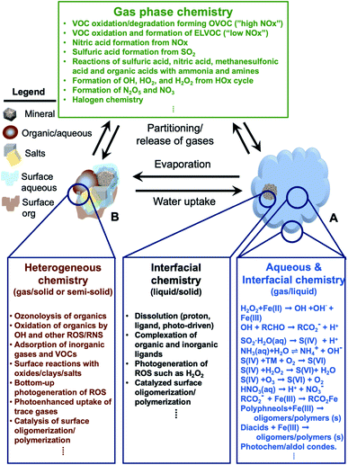 |
| | Fig. 2 Schematic diagram of reactions and processes that highlight chemical coupling in the atmospheric gas, particle and droplet phases. Day and night time gas phase chemistry leads to the degradation of VOCs, nucleation and growth of SOA, generation of reactive radicals, and transformation of NOx and SO2. Gas phase reactants and products can partition to cloud/fog droplet (A) or aerosol particles (B). The organic content in B could be from primary or secondary sources. A cloud/fog droplet (A) is a microreactor for bulk and heterogeneous chemistry at the liquid/solid or semi-solid and gas/liquid interfaces. Evaporation processes decrease the amount of liquid water in aerosol particles (B) leading to crystallization of salts and preferential ‘salting out’ of organics. Reactions in A and B can release gases as well. Abbreviations are: oxygenated volatile organic compounds (OVOCs), extremely-low VOC (ELVOC), and transition metals (TMs). | |
The objective of this review is to recount the current state of knowledge of the role of transition metals, iron in particular, in catalyzing reactions that lead to atmospheric BrC formation. Dust is a major source of iron in atmospheric aerosols74–78 because iron is the most abundant transition metal in the Earth's crust.79 Anthropogenic combustion80 including coal burning81,82 and biomass burning,83–85 in addition to brake wear,86 is found to contribute 50% of the total soluble iron deposited on the ocean.85,87,88 Single particle analysis of field-collected aerosols from the marine, urban and rural sites showed that they contain soluble and insoluble iron.85,89–99 Field studies reported the transport of transition metals including iron from the oceans to the atmosphere in the form of sea spray and metal enrichment at the interface of marine aerosols.100–102 An earlier review article focused on the chemical aging of atmospheric aerosols containing iron and organic matter, particularly those that model humic-like substances (HULIS).77 In that review, a recount of the literature was provided from field measurements and modelling studies of iron in aerosols, iron chemistry under dark conditions, photochemical reactions driven by iron obtained from bulk and surface-sensitive measurements, and molecular level differences between bulk and surface water that affect the reaction mechanisms. The scope of this review is to recount the recent results that highlight the role of iron in catalyzing soluble and insoluble atmospheric BrC formation by new and potentially important pathways. This review is organized into five main sections: iron in atmospheric aerosols, organic compounds in atmospheric aerosols, complexation and redox reactivity of iron with organics, case studies on iron-catalyzed insoluble and soluble BrC formation, and atmospheric impact. The review concludes with a summary and directions for future research.
2. Iron in atmospheric aerosols
The chemistry of iron species is rich under a wide range of atmospherically relevant conditions. The following sections elaborate on the sources of iron in atmospheric aerosol particles, atmospheric aging pathways that lead to iron solubilization, and soluble iron concentrations in aerosol liquid water.
2.1 Sources
Mineral dust from natural and anthropogenic sources is a major component of primary aerosols in the atmosphere with the estimated atmospheric loading and emission flux of 19.2 Tg and 1840 Tg year−1, respectively.73,103 On the other hand, global fluxes and mass loadings of AFCID have been severely under-represented in regional and global models, despite having surface PM2.5 measurement networks for emission inventories (see the Surface PARTiculate mAtter Network (SPARTAN), https://www.spartan-network.org). Philip et al.8 included AFCID emissions in a global simulation using GEOS-Chem. Fig. 3 shows the annual mean concentration of PM2.5 dust for 2014–2015: total dust (top panel), natural mineral dust (middle panel), and AFCID (bottom panel), as simulated with the GEOS-Chem model. Also shown in the top panel are circles for different locations that compare the mean measured PM2.5 dust from the SPARTAN in 2013–2015 (inner circles) with simulated values (outer circles). It was estimated that 2–16 μg m−3 of AFCID increases PM2.5 dust concentrations across East and South Asia.8 As noted by the authors, this concentration of simulated AFCID is comparable to that of natural mineral dust over parts of Europe and Eastern North America.8 Overall, dust particles provide surfaces for a range of chemical reactions with trace inorganic and organic species resulting in a change in the chemical composition and hygroscopic properties of these particles.55,73,78,104 The following section expands on dust aging in the atmosphere.
 |
| | Fig. 3 Annual mean (2014–2015) concentration of PM2.5 total dust (top panel), natural mineral dust (middle panel), and anthropogenic fugitive, combustion, and industrial dust (bottom panel) simulated with the GEOS-Chem model. Colored concentric circles in the top panel denote SPARTAN-measured campaign-mean (2013–2015) PM2.5 dust concentration (inner circle) and the coincident simulated value (outer circle). Reproduced from ref. 8 with permission from the Institute of Physics (IOP) Science Publishing, © The Author(s), 2017. | |
2.2 Atmospheric aging of mineral dust
The residence time of dust in the atmosphere during long range transport impacts the climate through affecting the surface temperature, wind, clouds, and precipitation rates.105 The long range transport increases the solubility of iron-containing minerals depending on their composition. The iron mineralogical composition varies from poorly crystalline to crystalline iron oxides to clay minerals depending on the source region.106 The ratio of crystalline hematite to the total of hematite and goethite is reported to vary with the geographical location. For example, for Asian dust, the ratio ranges from 0.32 to 0.37, whereas for North African dust from 0.29 to 0.63.106 The surface area was also found to be the predominant factor affecting iron solubility through acidic surface reactions.107 Asian108–110 and Saharan African dust111–114 have been shown to undergo extensive processing during long range transport that impact their mixing state and morphology.31 The uptake coefficients of OH, HO2, H2O2, O3, HCHO, HONO, NO3, and N2O5 on mineral dust particles and their proxies were reported to range from 10−6 to 0.2.115 Heterogeneous reactions of African mineral dust with VOCs were found to be irreversible for limonene and reversible for toluene.116
Acidic reaction conditions are commonly found in atmospheric aerosol particles, as well as in fog and cloud droplets, where soluble and insoluble iron species catalyze a number of chemical processes.77,117–119 In the presence of water soluble organic compounds, acidic reaction conditions can lead to secondary products.120 Freshly emitted dust particles contain more than one monolayer of adsorbed water over a wide relative humidity range.73 Surface reactions of dust with nitric and sulfuric acids lead to the formation of adsorbed nitrate and sulfate, which is enhanced in the presence of water.104 Photolysis of surface nitrate was reported to release NO2, which reacts with mineral dust to produce HONO.104,121 Near-neutral pH was also reported for cloud droplets.122 There have been no attempts to directly measure the pH of surface water in dust. Basic pH is typically measured in the slurries of unprocessed dust due to the presence of metals that act as Lewis acid sites.123
In addition, mixing with biomass burning products that include gases and aerosol particles also occur during the long range transport of dust.124,125 For example, Paris et al.126 reported that entrainment of dust deposited on vegetation makes biomass burning a significant indirect source of iron, where mixing with biomass burning aerosols enhances the solubility of iron. Li et al. in ref. 109 and 110 show electron microscopy images of aged sulfur-rich dust particles encapsulated with an organic film from either primary or secondary sources. In the same studies, soot particles were found to be internally mixed with sulfur- and iron-rich particles. These mixing states provide realistic scenarios for iron-catalyzed reactions to take place within or at the surface of dust particles.
The main two mechanisms that lead to iron release from dust and iron (oxyhydr)oxides are proton- and ligand-promoted dissolution.127–129 Laboratory and field studies from nearly four decades of research into these mechanisms showed that a number of variables play a role, namely the pH, particle size, degree of crystallinity, presence of solar radiation, and adsorption mode of Fe–organic complexes (i.e., structure of surface complexes).130–133 In general, the highest rates of dissolution occur under acidic conditions107,134 (pH < 4), in the presence of solar radiation and oxalate, with nanometer size and amorphous iron-containing particles. Also, UV irradiation of aqueous organic aerosol tends to fragment organic compounds producing smaller, more volatile compounds from larger oligomeric ones.135–137 Light-absorbing compounds derived from BBOA have also been found to fragment and photobleach under irradiated conditions.138 Such photodegradation processes can be amplified in the presence of Fe(III), which efficiently catalyzes photo-Fenton processes.139–146
2.3 Concentration of soluble iron
The concentration of iron in rainwater and fog, snow, and cloud waters from different locations was summarized by Deguillaume et al.119 The data show that the total and dissolved iron concentrations are location dependent and range from 0.1 to 1138 μM. Hence, a typical concentration of dissolved Fe(III) in cloud droplets (diameter ∼ 20 μm) is around 10−6 M.119 Therefore, for an aerosol particle produced by evaporation of cloud droplets down to a diameter of 1 μm, the concentration of dissolved Fe(III) could be as high as 10 mM. For example, Gen et al.147 measured iron concentrations in fine particles across China in the range 331–1640 ng m−3. To estimate the concentration of water soluble iron, they used the typical lower limit of iron solubility of 5%. The corresponding molar concentrations were calculated using an aerosol liquid water content of 6 × 10⁻⁸ L m−3 of air and found them to range from 5 to 43 mM. Since the reaction kinetics are affected by the concentration of reactants, exploring iron chemistry using micro- to millimolar levels would cover the range of reactions in aerosol to droplet nano- to micro-environments.
3. Organic compounds in atmospheric aerosols
Organic compounds represent a major fraction of atmospheric aerosol particles. Advances in the analysis of organic aerosol particles from primary and secondary sources have been the subject of a number of reviews.15–17 The organic content in atmospheric particles is characterized by a number of functional groups with the oxygen-to-carbon elemental ratio (O:C) ranging from 0.1 to 1.0 and are often grouped together into classes of compounds.35 Our latest study148 highlights that the knowledge of the pKa values of organic acids, some of which are currently incorporated in atmospheric chemistry models, is not enough to fully understand their complexation and reactivity with transition metals. The knowledge of structural effects on the kinetics of these reactions provides invaluable information of the role of the diacids in changing the chemical and physical properties of aerosol particles. Identifying functional groups in organic aerosol particles aid in understanding and predicting their chemical and photochemical reactivities. Examples of ‘offline’ techniques used to identify organic functional groups are Fourier transform infrared spectroscopy (FTIR) and nuclear magnetic resonance spectroscopy (NMR). The application of infrared spectroscopy to the detection and quantification of functional groups in water soluble organic particles from the smog chamber and field studies has been reviewed by Reggente et al.149 and Gao et al.150 The identification and quantification of functional groups in organic aerosol particles using NMR Spectroscopy was reviewed by Duarte and Duarte.39,151 Classes of identified organic functional groups include aliphatic, alkene, aromatic, and carbonyl carbon, in addition to alcohols, organosulfates and amines. The following two sections highlight two classes of organic compounds whose reactions with iron led to the formation of BrC: phenolic compounds and unsaturated dicarboxylic acids.
3.1 Phenolic compounds
Biomass burning is one of the largest sources of organics, gases and BBOA in the atmosphere, in general, and phenolic compounds, in particular. Examples of these phenolic compounds are catechol, guaiacol, resorcinol, and hydroquinone. The relative amounts of these compounds vary with fuel type152 and combustion conditions.153,154 Also, these compounds are produced by photo-oxidation of aromatic VOCs, are well-known aromatic SOA precursors, and are simple models for the aromatic fraction of HULIS in aerosol particles.155 Similar to atmospheric dust, BBOA travels long distances156 and hence there are realistic scenarios in which catechol and related compounds can end up in iron-containing particles. For example, primary particles from cooking emissions contain internally mixed soluble iron and organics.157 Smoke from biomass burning is often spread by wind, which also lifts crustal particles off the ground. Mineral dust is known to be transported globally by wind, which offers ample time for the partitioning of organic vapors into iron-containing particles.
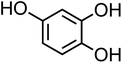
The simplest phenolic compounds are catechol and guaiacol. The gas phase concentration of catechol can be as high as 50 ppbv (∼5 × 10⁻⁸ atm), resulting from biomass burning, pyrolysis and combustion,158 but in most cases it will be well below the 1 ppbv (10−9 atm) level. With Henry's law constant of 8.3 × 10⁵ M atm−1,159 this translates into 41.5 mM and 0.83 mM, respectively, in a bulk system like a cloud droplet. The concentrations could be higher in the interfacial region of the particles because of surface enhancement of organics.160 Similar calculations could be done for guaiacol that has a Henry's law constant of 973 M atm−1 (ref. 161) and for other polyphenols listed in Table 1. As presented in the following sections, the reactivity of these compounds and their derivatives with iron proceeds differently because of their structure.
Table 1 Physical properties of selected semi-volatile phenolic compounds reactive with iron
| Compound name |
Structurea |
O:C molar ratio |
Molecular weighta (g mol−1) |
pKa ata 25 °C |
Henry's law constantb (M atm−1) at 25 °C |
|
From ref. 170–178.
From ref. 159, 161 and 179.
|
| Catechol (C6H6O2, CA) |

|
0.33 |
110.11 |
9.3, 12.6 |
8.3 × 10⁵ |
| 3-Hydroxycatechol (C6H6O3, 3-HC) |

|
0.5 |
126.11 |
9.0, 11.6, 14 |
6.4 × 10⁶ |
| 4-Hydroxycatechol (C6H6O3, 4-HC) |
|
0.5 |
126.11 |
9.1, 11.6, — |
— |
| 4-Nitrocatechol (C6H5NO4, 4-NC) |
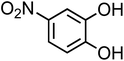
|
0.67 |
155.11 |
6.7, 11.3 |
∼106 |
| 4-Methylcatechol (C7H8O2, 4-MC) |
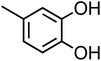
|
0.29 |
124.14 |
9.6, 14 |
— |
| Guaiacol (C7H8O2, GA) |

|
0.29 |
124.14 |
10 |
973 |
| Coniferaldehyde (C10H10O3, CON) |
|
0.3 |
178.18 |
9.7 |
— |
| Syringol (C8H10O3, SYR) |

|
0.38 |
154.16 |
9.8 |
1.2 × 10⁴ |
|
o-Cresol (C7H8O, o-CR) |

|
0.14 |
108.14 |
10.3 |
6.3 × 10² |
|
p-Cresol (C7H8O, p-CR) |

|
0.14 |
108.14 |
10.3 |
1.3 × 10³ |
| 2,4-Dinitrophenol (C6H4N2O5, 2,4-DNP) |
|
0.83 |
184.11 |
4.1 |
3.5 × 10³ |
3.2 Dicarboxylic acids
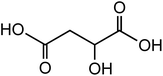
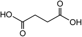
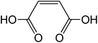
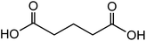
Dicarboxylic acids are abundant in atmospheric aerosols from continental, marine and polar regions with mass concentrations in tens to hundreds of ng m−3 of air.162Fig. 4 shows the gas phase and in-cloud oxidation processes responsible for their formation from natural and pollution-driven organic precursors. The most abundant diacid is oxalic acid (C2). Ubiquitous C3–C6 dicarboxylic acids such as malonic, malic, maleic, succinic, glutaric, fumaric and muconic acids are detected in BBOA aerosol particles163 and used in laboratory studies investigating liquid–liquid phase separation.35 Ring-opening reactions involving common atmospheric aromatic compounds, such as benzene, toluene, and xylenes, are known sources of unsaturated aldehydes164 and dicarboxylic acids.3 Muconic acid was identified as a product of photo-oxidation of benzene,165,166 and fumaric, maleic, and succinic acids are commonly observed in the atmosphere.167,168 These diacids, along with inorganic salts, influence the pH, ionic strength, water activity, and viscosity of the aerosol liquid water and also compete for binding to iron, specifically the anionic species.169 Using an aerosol liquid water content of 6 × 10⁻⁸ L m−3 of air, Gen et al.147 estimated the molar concentration of C2–C4 diacids to range from 3 to 95 mM depending on the diacid over a number of locations in China. Table 2 lists the physical properties of C2–C6 dicarboxylic acid that we used to explore their complexation with iron and their effect on the extent of BrC formation using catechol68,148 and in the absence of catechol.69 The following sections elaborate more on these cases.
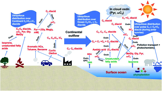 |
| | Fig. 4 Schematic representation of atmospheric reaction pathways of dicarboxylic acids and other related water-soluble organic compounds (Oxdn = photochemical oxidation). Adapted from ref. 162 with permission from Elsevier, © 2016. | |
Table 2 Physical properties of selected dicarboxylic acids
| Compound name |
Structurea |
O:C molar ratio |
Molecular weighta (g mol−1) |
pKa ata 25 °C |
Aqueous saturation concentrationb (wt%) at 25 °C |
|
From ref. 170.
From ref. 180 and 181.
|
| Oxalic acid (C2H2O4) |

|
2 |
90.03 |
1.3, 3.8 |
9.52 |
| Malonic acid (C3H4O4) |
|
1.33 |
104.06 |
2.83, 5.69 |
61.3 |
| Malic acid (C4H6O5) |
|
1.25 |
134.09 |
3.40, 5.11 |
57.4 |
| Succinic acid (C4H6O4) |
|
1 |
118.09 |
4.16, 5.61 |
7.2 |
| Fumaric acid trans-C4H4O4 |

|
1 |
116.07 |
3.0, 4.2 |
0.7 |
| Maleic acid cis-C4H4O4 |
|
1 |
116.07 |
1.9, 6.2 |
44.1 |
| Glutaric acid (C5H8O4) |
|
0.8 |
132.12 |
4.31, 5.41 |
58.8 |
| Muconic acid (trans, trans-C6H6O4) |

|
0.67 |
142 |
3.9, 4.7 |
Not determined |
4. Complexation and redox reactivity of iron with organics
The chemical state (e.g., soluble vs. insoluble) and cycling of iron between oxidation states 3+ and 2+ depend on a number of chemical processes that include complexation strength to organic and inorganic ligands, the presence of electron donors/acceptors, and absorption kinetics of UV-vis light. The following sections elaborate on these topics beyond what was covered in the earlier review.77
4.1 Soluble organic complexes with iron
Acidic and phenolic functional groups are strong complexing agents to soluble iron.77 Visual MINTEQ freeware is a chemical equilibrium computer program with extensive thermodynamic databases that allow for the calculation of speciation, solubility, and equilibrium of solid and dissolved phases of minerals in an aqueous solution.182 Visual MINTEQ has a large selection of organic acids and includes a database management tool that allows organic species to be easily added or deleted. It could be used as a tool to obtain values for the pKa and complex stability constants (logK). Also, this program can generate the relative concentration of different species that exist in solution at equilibrium. Fig. 5 shows examples of iron speciation curves in solution mixtures containing iron chloride, oxalic acid and ammonium sulfate as a function of pH.68 These curves are very useful in quantifying dominant species at a given pH for accurate interpretation of chemical and photochemical reactivity in multicomponent systems.
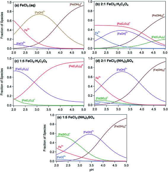 |
| | Fig. 5 Speciation curves of iron chloride, oxalate, and sulfate with variable molar ratios. Ratios in headings are mol:mol. The curves were generated using equilibrium constants for the acid dissociation and complexation reactions of iron from the database in Visual MINTEQ, v. 3.1. Reproduced from ref. 68 with permission from the American Chemical Society, © 2019. | |
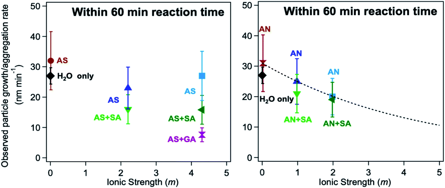
The logK values of different iron complexes can be used in the interpretation of experimental data in multicomponent systems, as illustrated in the following sections. Reliable kinetic studies on iron complex formation with the organic ligands of atmospheric relevance are sparse. Table 3 lists values for the forward complex formation rate constants, kf, between FeOH2+ and selected aliphatic carboxylic acids for comparison with catechol. Within the experimental conditions listed in Table 3, the kf value for forming the iron catecholate complex, Fe(C6O2H4)+ (Fe–CA), is 3× that for forming iron sulfate, Fe(SO4)2−, and iron malate, Fe(C4O5H4)+ (Fe–MA). As described in detail in Section 5, iron-catalyzed polymerization of catechol forming insoluble black polycatechol particles and colored water-soluble oligomers occurs in systems containing excess ammonium sulfate (AS)/nitrate (AN) and C4–C5 dicarboxylic acids, which were used to vary the ionic strength under acidic pH (∼2).148
Table 3 Literature values for the complex formation rate constant between FeOH2+ and selected ligands. Reproduced from ref. 148 with permission from the American Chemical Society, © 2021
| Reaction |
Experimental conditions |
Forward rate constant, kf (M−1 s−1) |
Ref. |
| Citric acid |
20 °C, [HClO4] = 0.01–0.05 M, pH = 1–2 |
50–930 |
183
|
| Oxalic acid |
25 °C, 1 M HClO4, ‘acidic’ pH |
2 × 10⁴ for FeOx+ |
184
|
| Sulfate |
25 °C, 1 M NaClO4, pH = 0.7–2.5 |
1 × 10³ for Fe(SO4)2− |
185
|
|
DL-Malic acid |
25 °C, 1 M NaClO4, pH = 1–2 |
95–103 |
186
|
| Catechol |
25 °C, 1 M NaClO4, pH = 1–2 |
3 × 10³ for FeCA+ |
187
|
4.2 Redox reactivity of iron forming soluble products
The presence of Fe(III)/Fe(II) species in aerosol particles can influence their oxidative potential through acting as electron acceptors/donors, respectively. The term “oxidative potential” refers to metal-driven redox chemical reactions that lead to the formation of reactive oxygen species (ROS), such as OH and H2O2, and also organic radicals/cations.188 The redox reactions catalyzed by iron not only can cause degradation of water-soluble organics but also the formation of soluble and insoluble secondary and high molecular weight organics depending on the chemical structure of the organic precursors.68–70,77,120,148,189–191
Under oxic conditions, Fe(III) species are dominant. Using basic principles of electrochemistry, one can predict if a redox reaction will take place spontaneously upon mixing Fe(III) with organic compounds acting as electron donors. In systems containing Fe(III), reduction reactions of iron species under acidic conditions are listed in Table 4 along with the reduction potential, E. Table 5 lists the oxidation potential and major products of phenol, catechol and guaiacol from electrochemical studies under acidic conditions.
Table 4 Selected reduction reactions of Fe species and their electrochemical potentials from ref. 192
| Rxn# |
Reduction reaction |
pH range |
E (V) range and pH dependency |
| 1 |
Fe(III) + e → Fe(II) |
0–2.12 |
0.77 |
| 2 |
Fe(OH)2+ + H+ + e → Fe(II) + H2O |
2.12–3.48 |
0.9–0.06 pH (pH 3, E = 0.72 V) |
| 3 |
Fe(OH)2+ + 2H+ + e → Fe(II) + H2O |
3.48–6.30 |
1.10–0.12 pH (pH 4, E = 0.62 V; pH 5, E = 0.5) |
Table 5 Electrochemical oxidation potential and reaction products of selected phenolic compounds
| Compound |
Oxidation potential (V) |
Cyclic voltammetry experimental conditions |
Oxidation reaction |
Ref. |

|
∼1 (pH 0.2–2) |
50 mV s−1vs. Ag/AgCl 0.5–25 mM Pt electrode |
|
193 and 194 |

|
0.43 → 0.2 (pH 4 → 8) |
50 mV s−1vs. Ag/AgCl 1 mM Pt electrode |
|
194 and 195 |

|
0.48–0.9 (pH 2) |
100 mV s−1vs. Ag/AgCl 0.1 mM boron-doped diamond electrode |
|
196
|
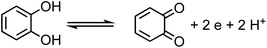
For a system containing catechol/Fe(III) at pH 3, eqn (1) and (2) represent the redox coupling for the net reaction shown in eqn (3):
Oxidation:
| | | Catechol → ortho-quinone + 2e + 2H+, Eox1 = 0.4 V | (1) |
Reduction:
| | | 2Fe(OH)2+ + 2H+ + 2e → 2Fe(II) + 2H2O, Ered = 0.72 V | (2) |
Net reaction:
| | | Catechol + 2Fe(OH)2+ → o-quinone + 2Fe(II) + 2H2O, Enet = Ered − Eox = 0.72 − 0.4 = 0.32 V | (3) |
The net positive redox potential indicates that reaction (3) is spontaneous under acidic conditions. Using the same approach, it could be concluded that redox reactions between phenol and Fe(III) are non-spontaneous under acidic conditions, whereas they are with guaiacol. The oxidation potential of a number of carboxylic acids of atmospheric relevance is higher than 1 V under acidic conditions. Hence, no spontaneous redox reactions take place with Fe(III) in solution.197
In addition, binding of Fe(III)/Fe(II) to polyphenols containing the catecholate or gallate (i.e., 3-HC in Table 1) moieties plays a role in their antioxidant properties.198,199 Complexes with Fe(II) quickly oxidize in the presence of oxygen in a process referred to as auto-oxidation to give Fe(III)–polyphenol complexes. Once these complexes form, the polyphenol can reduce Fe(III) to Fe(II) forming a semiquinone that further oxidizes to a quinone. If the organic ligands exist in excess, the coordination of two or three polyphenol ligands inhibits Fe(III) reduction processes.198 As shown below in Section 5, irreversible oxidative polymerization reactions take place in systems with excess Fe(III) forming insoluble black particles, and the particle density depends on the organic ligand to iron molar ratios.
5. Case studies on iron-catalyzed insoluble and soluble BrC formation
The results on iron research to date summarized above are invaluable in understanding and predicting the chemical reactivity of dust aerosols. However, the role of dust in catalyzing the polymerization reactions of organics due to the soluble iron fraction and its effect – as a dust aging pathway – on the optical properties and the ice nucleation efficiency have received little attention under atmospherically relevant conditions. These reactions might be as efficient as those producing BrC from VOC precursors.33 In the following sections, the results to date from our group and others show that iron can catalyze the oligomerization and polymerization reactions of phenolic compounds and some dicarboxylic acids in systems that model aerosol particles.
5.1 Phenolic precursors
5.1.1 Catechol and guaiacol.
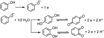
The phenolic compounds that have been tested to date for the reaction with soluble Fe(III) under acidic conditions and formed colored oligomeric and polymeric products over short periods of time (i.e., 2 h) are the majority of those listed in Table 1. Slikboer et al.70 reported the first set of experiments on the efficient formation of highly absorbing, water-insoluble particles of polycatechol and polyguaiacol from the reaction of Fe(III) at pH 3 with catechol and guaiacol at millimolar concentrations. Fig. 6 shows the digital photos of the unfiltered solutions as a function of time, dry particles collected on filters, and the UV visible spectra of reaction solutions. Both catechol and guaiacol solutions are transparent in the visible range and show a UV band around 274 nm due to π → π* transitions in the benzene ring. The UV-vis absorbance spectrum of FeCl3 solution (pale yellow) shows a band around 295 nm from the ligand-to-metal-charge transfer (LMCT) of the prevailing species in solution, [Fe(H2O)5OH]2+.200 Spectra collected at pH = 1–5 exhibit a shift in this peak because the iron speciation is strongly pH-dependent.201 In the case of catechol, an initial green color was observed for the 1:2, 1:1 and 2:1 organic reactant:Fe molar ratios, which was attributed to the formation of a bidentate mononuclear catechol–Fe complex with an LMCT band around 700 nm.202 The intensity of this feature varied with the amount of Fe in the solution mixture: the lowest intensity was observed for the 2:1 organic reactant:Fe solution mixtures. The intense spectral feature at 390 nm was attributed to n → π* transitions of o-quinone species formed from the oxidation of catechol–Fe complexes.203 This peak was also observed at lower concentrations of catechol and iron under acidic conditions and for other catecholates such as gallic acid.200 The presence of –OCH3 group in the case of guaiacol inhibited the formation of the iron complex, as evident by the absence of the characteristic LMCT band in Fig. 6f. As explained below, the spectra in Fig. 6f indicated the formation of soluble amber-colored oxidation products due to iron redox chemistry.
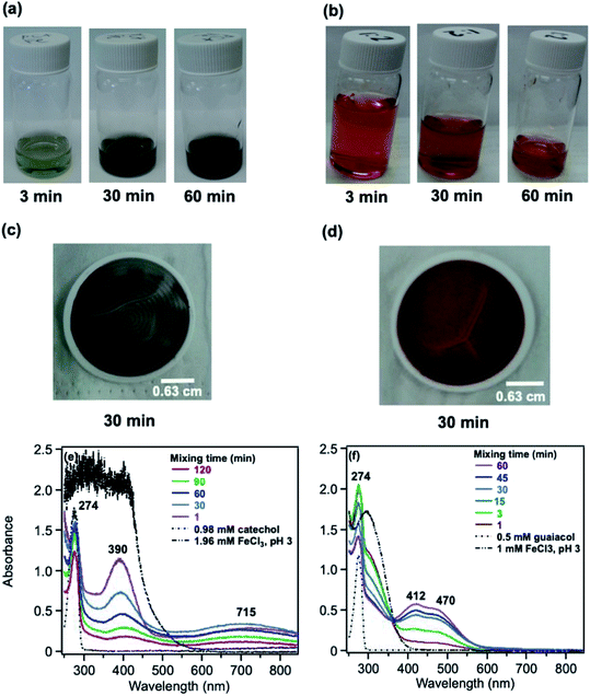 |
| | Fig. 6 Dark reaction of catechol and guaiacol with FeCl3 at pH 3: (a and b) digital images of the 1:2 organic reactant/Fe molar ratio of unfiltered solutions as a function of time; (c and d) particles on filter after 30 min; and (e and f) the corresponding UV-vis spectra after filtration. Reproduced from ref. 70 with permission from the American Chemical Society, © 2015. | |
The data in Fig. 6 clearly show the phase separation and solid particle formation in water. Fig. 7 shows scanning electron microscopy (SEM) images of the particles collected on the filters in Fig. 6. These images clearly show micron-size conglomerates of nanometer-size soot-like particles that we named ‘fireless soot’. Energy dispersive X-ray spectroscopy (EDS) experiments showed that polycatechol and polyguaiacol particles are organic materials with no detectable iron content. The mass yield experiments using a 1:2 organic reactant:Fe molar ratio at pH 3 after 2 h of reaction were 47 ± 4% and 49 ± 14%, for polycatechol and polyguaiacol, respectively. These mass yield values were calculated using eqn (4):
| |  | (4) |
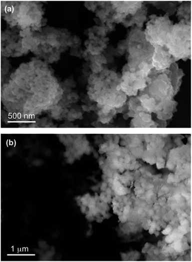 |
| | Fig. 7 SEM images of (a) polycatechol and (b) polyguaiacol collected on copper grids after a 90 min dark reaction of catechol with FeCl3 at pH 3 in a 1:2 molar ratio. Reproduced from ref. 70 with permission from the American Chemical Society © 2015. | |
These mass yield values are comparable to or larger than the typical mass yields of SOA obtained by the photo-oxidation of common VOCs, such as terpenes,204 and are also larger than the yields associated with aqueous SOA (aqSOA) photochemical production.205 Therefore, the iron-catalyzed reactions of catecholates have high potential to produce SOA with superior efficiency.
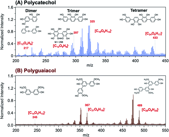
Using Matrix Assisted Laser Desorption Ionization Time-of-Flight Mass Spectrometry (MALDI-TOF-MS), Link et al.206 explored the structure of a polycatechol thin film in the m/z range 200–450 (Fig. 8A). The MALDI mass spectrum in the m/z range 200–550 for a polyguaiacol thin film sample is shown for comparison in Fig. 8B. The tentative assignment of the peaks to chemical formulae and structures of oligomeric fragments is also shown in Fig. 8. While the peak pattern is complex, the highest intensities were associated with the trimer (around m/z 330 and 370) and the tetramer species (around m/z 430 and 490). Higher order oligomers, above m/z 450, were not reproducibly observed. In the following sections, a summary of previous studies is provided on the analysis of organic solvent extracts of polycatechol and polyguaiacol that contained oligomers with masses observed in the MALDI spectra. These structural details are useful when comparing the hygroscopic properties and ice nucleation activity of polycatechol and polyguaiacol with other organics.73
 |
| | Fig. 8 Representative MALDI-TOF mass spectrum of (A) polycatechol and (B) polyguaiacol thin films in the negative ion reflector mode, [M–H]−. The structure of fragments was based on ref. 207 for polycatechol and ref. 208 for polyguaiacol. No additional matrix compound was used in the spectra collection. Spectra were collected with the assistance of Dr Lauren T. Fleming, Prof. Sergey A. Nizkorodov, and Dr Ben Katz at the University of California Irvine Mass Spectrometry Facility. | |
Moreover, Fig. 9 shows the attenuated total internal reflectance FTIR (ATR-FTIR) spectra of solid polycatechol and polyguaiacol formed in reactions of Fe(III) with catechol and guaiacol. The 2000–1000 cm−1 spectral range contains vibrations of aromatic (1640–1400 cm−1), C–O and C–C stretching (1400–1200 cm−1) and C–H bending (1200–1000 cm−1) modes. The spectrum of polycatechol recorded by transmission FTIR using KBr pellets209,210 is in line with the one shown in Fig. 9, where broadening and shift in peak frequencies were observed due to the rigid structure of polymers. The high intensity of features in the 1400–1200 cm−1 range is characteristic of phenylene (C–C) and oxyphenylene (C–O–C) linkages. These spectra show no absorbance around 1700 cm−1, indicative of carbonyl (C![[double bond, length as m-dash]](https://www.rsc.org/images/entities/char_e001.gif) O) groups, which were reported for catechol and guaiacol SOA due to reaction with ozone.155 The following sections highlight the effect of ring substituents in the benzene rings of catechol and guaiacol and competing ligands on the iron-catalyzed oxidative polymerization of catechol and guaiacol.
O) groups, which were reported for catechol and guaiacol SOA due to reaction with ozone.155 The following sections highlight the effect of ring substituents in the benzene rings of catechol and guaiacol and competing ligands on the iron-catalyzed oxidative polymerization of catechol and guaiacol.
 |
| | Fig. 9 ATR-FTIR absorbance spectra of (a) solid polycatechol (bottom) and polyguaiacol (top) deposited on a ZnSe ATR crystal from a water/ethanol slurry, followed by drying overnight. Reproduced from ref. 70 with permission from the American Chemical Society, © 2015. | |
5.1.2 Derivatives of catechol and guaiacol.
The reactions of Fe(III) with catechol and guaiacol derivatives were investigated by Chin et al.190 to explore the effect of ring substituents on the polycatechol and polyguaiacol formation efficiency. These derivatives are listed in Table 1, which include 4-hydroxycatechol (4-HC), 3-hydroxycatechol (3-HC), coniferaldehyde (CON), 4-methylcatechol (4-MC), 4-nitrocatechol (4-NC) and 2,4-dinitrophenol (2,4-DNP).68–70,211Fig. 10A shows the UV-vis spectra of reaction mixtures as a function of time along with digital photographs of the reaction solutions. In these experiments, the concentration of soluble Fe(III) was less than or equal to 2 mM, which is a relevant choice for aerosol particles, as stated above. Fig. 10B shows digital photographs of the filters with insoluble products after 2 h of reaction time with CA, 3-HC, 4-HC, and CON. 3-HC and 4-HC are catechol derivatives with an extra hydroxyl group in the para- and meta-positions, respectively. The UV-vis spectra indicated the formation of quinone species between 350 and 400 nm. Both compounds formed colored particles with mass yields of 27 ± 2% and 32 ± 3% for 3-HC and 4-HC, respectively, after 2 h of reaction with Fe(III) at pH 3. The reaction of 4-MC and FeCl3 did not produce particles over the 2 h reaction time. However, particles did eventually appear on the filter after allowing the mixture to react further for 24 h. On the other hand, the reaction of Fe(III) with 4-nitrocatechol and 2,4-dinitrophenol did not form particles.190
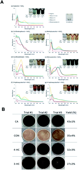 |
| | Fig. 10 (A) UV-vis absorption spectra of mixtures of Fe(III) with (a) CA, (b) 2,4-DNP, (c) 4-MC, (d) CON, (e) 4-NC, (f) 3-HC, and (g) 4-HC. Different colors of traces correspond to spectra of organic reactants before mixing (red), 1–5 min after mixing (orange), 1 h after mixing (green), 2 h after mixing (blue), and filtered solution (purple). The final concentration of organics is 1 mM, and the final concentration of Fe(III) is 2 mM. The photographs are those of unfiltered solutions. (B) Photographs of filters containing particles after 2 h of reaction, filtration, and drying for CA, CON, 4-HC, and 3-HC. The last column contains the average (n = 3) effective mass yield in percent. Reproduced from ref. 190 under Create Commons License (CC BY-NC) from the Royal Society of Chemistry, © The Author(s), 2021. | |
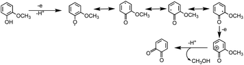
In the case of the guaiacol derivative, CON, particles formed after 2 h reaction with iron with a mass yield of 35 ± 4%. These differences in the reactivity of catechol and guaiacol derivatives with iron are discussed in the following sections. Syringol (SYR) is another guaiacol derivative, and its reactivity with iron was investigated by Lavi et al.211. They reported the formation of insoluble brown to black matter that was collected on a filter, washed and then completely dissolved in dimethyl sulfoxide (DMSO) and analyzed using UV-vis spectroscopy and liquid chromatography/mass spectrometry (see sections below for details). The insoluble matter was also analyzed using X-ray photoelectron spectroscopy (XPS), which showed that the surface chemical composition was predominately carbon (76–87%), as evidenced from the peaks of CC or C–H, C–OH, and CO functional groups. The atomic concentration of oxygen ranged from 13 to 24%. The following sections provide details on the mechanism that explains iron-catalyzed polymerization of phenolic compounds.
5.1.3 Mechanism of iron-catalyzed oxidative polymerization.
5.1.3.1 Insoluble polycatechol formation.
Abiotic oxidative polymerization of phenolic compounds is catalyzed by transition metals such as iron. Scheme 1 shows a proposed mechanism for polycatechol formation based on the results from ref. 212–216 under dark conditions leading to the formation of oligomers and polymeric particles. Iron catalyzes the deprotonation of catechol and its derivatives below their first pKa198 and forms strong bidentate complexes with stability constants that vary with iron species in solution. For example, the formation of Fe(C6O2H4)+ as per eqn (5) and (6) has logK values of 7.9 and 9.9 depending on the iron species:| | | Fe3+ + H(C6O2H4)− ⇌ Fe(C6O2H4)+ + H+ | (5) |
| | | FeOH2+ + H(C6O2H4)− ⇌ Fe(C6O2H4)+ + H2O | (6) |
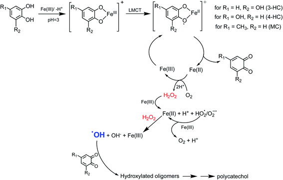 |
| | Scheme 1 Suggested mechanism for polycatechol formation. Reproduced from ref. 190 under Create Commons License (CC BY-NC) from the Royal Society of Chemistry, © The Author(s), 2021. | |
The extent of charge transfer that oxidizes the organic compound and reduces Fe(III) depends on the benzene ring substituents. In this mechanism, dissolved O2 is the oxidant and Fe(III) plays a role as a catalyst. Tran et al.69 investigated the effect of dissolved oxygen in aqueous solutions containing iron under acidic conditions. The level of dissolved O2 in these experiments was quantified at 11 ± 2 mg L−1 (or ppm). Bubbling N2 gas into the reactant solutions (prior to mixing) for 1 h reduced the level of dissolved O2 to 3 ± 2 ppm. Longer bubbling times up to 2 h did not significantly reduce this value further. So, we concluded that it is practically impossible to completely purge dissolved oxygen by nitrogen bubbling, and that the amount of dissolved oxygen below the detection limit of the measuring electrode is enough to oxidize polyphenols in the presence of iron.
Cycling between Fe(II) and Fe(III) species is coupled with the production of ROS, H2O2, and OH radicals as intermediates.217 The LMCT steps lead to the formation of quinone species and the release of Fe(II). Oxidation of Fe(II) to Fe(III) by dissolved oxygen is spontaneous according to reactions (7)–(9):
| | | Fe(II) → Fe(III) + e, Eox = −0.75 V | (7) |
| | | O2(g) + 2H+ + 2e → H2O2(l), Ered = +0.7 V | (8) |
Net reaction:
| | | Fe(II) + 2H+ + O2(g) → Fe(III) + H2O2(l), Enet = Ered − Eox = +1.45 V | (9) |
The rate constant for the net spontaneous oxidation of Fe(II) by dissolved oxygen is pH-dependent and is known up to pH 6.218 Another pH-dependent reaction of Fe(II) with O2(g) produces the superoxide anion, O2˙−, according to:
| | | Fe(II) + O2(g) → Fe(III) + O2˙−, k = 107 M−1 s−1 (ref. 119) | (10) |
The pKa of the superoxide is 4.8 and its protonated form is HO2˙.219 Under excess Fe(III), the formation with H2O2 or HO2˙/O2˙− from the above reactions occur according to eqn (11) and (12):
| | | Fe(III) + H2O2(l) → Fe(II) + HO2˙/O2˙− + H+, k = 2 × 10⁻³ M−1 s−1 (ref. 220) | (11) |
| | | Fe(III) + HO2˙/O2˙− → Fe(II) + O2 + H+, k = 7.8 × 10⁵ M−1 s−1 (ref. 220) | (12) |
The in situ formation of Fe(II) and H2O2 would lead to the OH radical production per the Fenton reaction shown in eqn (13) under acidic conditions:
| | | Fe(II) + H2O2(l) → Fe(III) + OH + OH−, k = 55 M−1 s−1 (ref. 220) | (13) |
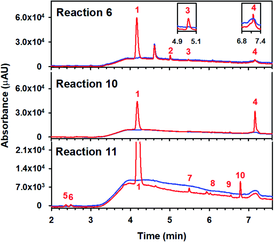
The rate of the Fenton reaction is pH-dependent, and the relative importance of the different elementary steps varies with the relative amounts of Fe(II) and H2O2 in solution.221 The OH radical in the presence of quinone and catechol species leads to hydroxylation of the benzene rings forming oligomers and eventually polycatechol. The formation of polycatechol in solution falls under the category of ‘mechanisms for polymerization reactions’, which are composed of three main steps: initiation, propagation and termination.222 The OH radical plays a role in the first and second steps. Under conditions characteristic of viscous multicomponent aerosol systems with relatively high ionic strength (I = 1–12 m) and acidic pH (∼2) that likely affected the kinetics of the polymerization reactions, Al-Abadleh et al.148 detected colored water-soluble oligomers shown in Scheme 2 using ultrahigh pressure liquid chromatography coupled with mass spectrometry (UHPLC-MS).
 |
| | Scheme 2 Structure of molecules and oligomers and their characteristic absorption wavelength detected in the reaction of catechol with Fe(III) under conditions characteristic of viscous multicomponent aerosol systems with relatively high ionic strength (I = 1–12 m) and acidic pH (∼2) using UHPLC-MS. Modified from ref. 148 with permission from The American Chemical Society, © 2021. | |
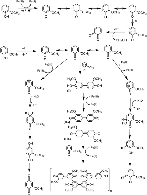 |
| | Scheme 3 Mechanism for the oxidation of guaiacol in the presence of excess iron under dark conditions leading to the formation of dimers and eventually polyguaiacol based on the mechanism reported in ref. 223 and 224. Reproduced from ref. 190 under Create Commons License (CC BY-NC) from the Royal Society of Chemistry, © The Author(s), 2021. | |
 |
| | Fig. 11 (Upper panel) HPLC/PDA chromatogram of guaiacol/Fe(III) reaction products. The x-axis is the retention time, the y-axis is the UV-vis absorption wavelength, and color denotes the intensity of the absorption signal. (Lower panels) UV-visible spectra of selected chromophores. The figure and the caption were reproduced from ref. 211 with permission from the American Chemical Society, © 2017. | |
Hence, based on the above, in situ reduction of Fe(III) to Fe(II) leads to the formation of phenoxy radicals, which proceeds through C–C radical coupling from compound I in Scheme 3. Compounds IIa and IIb (Scheme 3) give rise to the spectral features at 412 and 470 nm (Fig. 6f), which were observed to decrease in intensity upon overnight storage of solutions.224,225 As detailed below, formation of these polymeric species has implications on the overall optical properties and chemical reactivity of the surfaces coated by these products.
5.1.4 Effect of competing ligands on the polycatechol and polyguaiacol formation efficiency.
5.1.4.1 Oxalate.
Oxalic acid (pKa 1.3 and 3.8)170 is a ubiquitous component and the most abundant dicarboxylic acid in ambient aerosols with a high complexation affinity to iron. The work by Kundu et al.163 on biomass burning aerosols showed that 77% of oxalic acid is formed from the degradation of dicarboxylic acids and related compounds, and 23% are likely directly emitted or chemically produced from other unknown precursors. Other well-studied mechanism of oxalate formation in atmospheric aqueous particles is the oxidation of glyoxal and methylglyoxal.226 Recently, Zhang et al.227 reported results from field measurements, showing enhanced formation of oxalate associated with iron-containing particles. They attributed this observation to the complexation of oxalate to iron following gas–particle partitioning of oxalic acid. In general, aqueous phase oxalate is the most effective organic compound among the known atmospheric organic ligands that promotes dust iron solubility.132
The thermodynamic stability constants of iron oxalate complexes were calculated using Visual MINTEQ software and found to vary with pH (Fig. 5b and c). In the pH range 2–3, the dominant iron species are Fe3+ and FeOH2+, which complex with hydrogen oxalate, HC2O4−, according to eqn (14) and (15):
| | | FeOH2+ + HC2O4− ⇌ Fe(C2O4)+ + H2O, logK = 6.9 | (14) |
| | | Fe3+ + HC2O4− ⇌ Fe(C2O4)+ + H+, logK = 4.9 | (15) |
In excess oxalate at pH 3, the following reactions also take place since a maximum of three oxalate molecules can complex with a single iron centre:
| | | FeOH2+ + 2HC2O4− ⇌ Fe(C2O4)2− + H2O + H+, logK = 8.9 | (16) |
| | | FeOH2+ + 3HC2O4− ⇌ Fe(C2O4)33− + H2O + 2H+, logK = 8.9 | (17) |
| | | Fe3+ + 2HC2O4− ⇌ Fe(C2O4)2− + 2H+, logK = 6.9 | (18) |
| | | Fe3+ + 3HC2O4− ⇌ Fe(C2O4)33− + 3H+, logK = 6.9 | (19) |
The left panel in Fig. 12 shows the effect of varying the amounts of oxalate, catechol and guaiacol on the mass of the insoluble product following 2 h reaction of these ligands with iron under dark conditions at pH 3.68 In the presence of equimolar amounts of oxalate and catechol, no suppression of particle formation was observed relative to the control experiments (absence of oxalate and sulfate), which corresponds to mass yields of ∼50% and 60% for polycatechol and polyguaiacol, respectively. The data also show a larger reduction in particle mass with guaiacol than catechol. Suppression of particle formation was observed with excess oxalate (left side of 2:1:1 Fe:catechol:Ox molar ratio, Fig. 12a). This suppression is explained by the predominance of soluble iron oxalate complexes, Fe(C2O4)2− and Fe(C2O4)33−. The logK values for the formation of both complexes equal 8.9 with FeOH2+ species, which is much higher than that for the ligand exchange between catecholate, H(C6O2H4)−, and Fe(C2O4)2− or Fe(C2O4)33− (logK = 1). Particle mass is also lower in the 1:1:1 Fe:catechol:Ox molar ratio (right side of 2:1:1, Fig. 12a). This observation is explained by the reduction in the rate of the oxidative polymerization reaction when iron is the limiting reagent relative to catechol, as highlighted in the above section Mechanism of iron-catalyzed oxidative polymerization.
 |
| | Fig. 12 Effect of adding oxalate (Ox, left) and ammonium sulfate (AS, right) on product mass after 2 h of dark aqueous phase reaction of 1 mM catechol and guaiacol with FeCl3 (total volume = 20 mL). The error bars represent the standard deviation (±σ) from averaging 3–4 filter weight values. The horizontal dashed line is the product mass for the control reaction (no added oxalate or sulfate) for 2:1 Fe:organic molar ratio. The figure and the caption were modified from ref. 68 with permission from the American Chemical Society, © 2019. | |
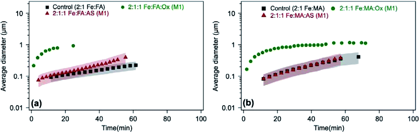
The time-dependent average particle size of polymeric particles produced in situ from the reaction of Fe(III) with aromatic reagents in the presence or absence of oxalate (and sulfate) in solution is shown in Fig. 13. Within the first 20 min, adding oxalate and sulfate leads to the formation of polycatechol particles in solution that are 2 and 2.5 times larger than those from control experiments, respectively (Fig. 13a). In light of the product mass yields obtained from filter weighing, one can take the interpretation of the DLS measurements further. For example, since the 2:1:1 Fe:catechol:Ox or AS reaction produces the same product mass as 2:1 Fe:catechol control (Fig. 12a and b), but the particles are initially larger (Fig. 13a), there must be fewer of them in the solution. This could indicate that the initial solution nucleation is retarded by oxalate, but once particles form they grow faster. When the reaction is carried out according to method 2 using sulfate (defined in the caption of Fig. 13), the DLS measurements show micron-size particles forming right away (Fig. 13a) with polydispersity index (PDI) above 0.5, indicating their high degree of polydispersity. As detailed above, the product mass from this reaction is double the control value at pH 3 (Fig. 12a). Hence, these combined results suggest the formation of larger and heavier particles in solution when iron sulfate is reacted with catechol according to method 2.
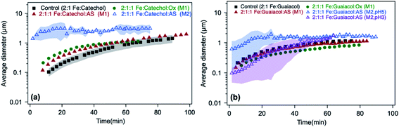 |
| | Fig. 13 Effect of adding oxalate (Ox) and ammonium sulfate (AS) on particle size from time-dependent DLS measurements during the dark aqueous phase reaction of (a) catechol (1 mM) and (b) guaiacol (0.5 mM). This molar ratio results in the maximum product mass per data shown in Fig. 1. ‘M1’ stands for method 1, where organic reagents were mixed first with AS or Ox, then the reaction time started when Fe was added. ‘M2’ stands for method 2, where AS or Ox were reacted first with Fe for 2 h, then the reaction time started when the organic reagent was added. The shaded areas represent the standard deviation of three trials. Unshaded data represent the average of two trials, with a standard deviation the size of the marker width (15%). The figure and the caption were modified from ref. 68 with permission from the American Chemical Society, © 2019. | |
In the case of guaiacol, particles produced according to method 1 (defined in the caption of Fig. 13) at pH 3 show no significant difference in size when oxalate (or sulfate) was added relative to the control (Fig. 13b). These conditions produce less product mass than the control per data in Fig. 12b. However, the cases that produced twice the product mass when sulfate was added according to method 2 at pH 5 and 3 resulted in higher variability in particle size within the first 40 min of reaction time. Similar to the results with catechol, these particles have a PDI above 0.5, indicating their high degree of polydispersity. When these results are combined with product mass results, they suggest the formation of fewer and heavier particles in solution when iron sulfate was reacted with guaiacol according to method 2. This method is more atmospherically relevant over a range of multicomponent aerosol processing than method 1. The results described above show a new role for oxalate in aerosol chemistry, given its higher concentrations than iron and organic reagents, which is to efficiently suppress secondary particle formation in solution.
5.1.4.2 Sulfate.
Sulfate is one of the most abundant inorganic components in aerosol particles that is mainly formed from aqueous phase oxidation of SO2, a process often catalyzed by soluble iron.117 Sulfate is routinely measured and incorporated in thermodynamic models that calculate the aerosol pH.228 Yu et al.229 reported a correlation between the sulfate and oxalate contents in particles and suggested a dominant in-cloud processing pathway to explain the close tracking of both species. Non-sea salt sulfate (nss SO42−) from anthropogenic sources were also reported to largely control the formation of water soluble SOA dominated by oxalate via aqueous phase photochemical reactions.230
The thermodynamic stability constants of iron sulfate complexes were calculated using Visual MINTEQ software and found to vary with pH (Fig. 5d and e). In the pH range 2–3, the dominant iron species are Fe3+ and FeOH2+, which complex with sulfate, SO42−, according to eqn (20) and (21):
| | | FeOH2+ + SO42− + H+ ⇌ FeSO4+ + H2O, logK = 6.3 | (20) |
| | | Fe3+ + SO42− ⇌ FeSO4+, logK = 4.3 | (21) |
In excess sulfate at pH 3, the following reactions also take place since a maximum of two sulfate molecules can complex with a single iron centre:
| | | FeOH2+ + 2SO42− + H+ ⇌ Fe(SO4)2− + H2O, logK = 7.4 | (22) |
| | | Fe3+ + 2SO42− ⇌ Fe(SO4)2−, logK = 5.4 | (23) |
The above logK values for the formation of soluble iron sulfate are lower than those for iron catecholate, Fe(C6O2H4)+ (9.9, reactions (5) and (6). These logK values explain the trend in product mass in Fig. 12b, where adding sulfate had no effect on particle formation in solution because [FeOH]2+ species are still the dominant species in solution (Fig. 5d and e). Under excess sulfate, an increase in the concentration of [FeSO4]+ relative to [FeOH]2+ species is observed at pH 3 (Fig. 5e). Data in Fig. 12b show that the product mass nearly doubled when the reaction resulting in the 2:1:1 Fe:catechol:AS molar ratio was carried out at pH 3 according to method 2 (i.e., catecholate reacts with iron sulfate complexes). Ligand exchange between catecholate and iron sulfate complexes is favorable with logK = 3.6, according to reaction (24):
| | | H(C6O2H4)− + FeSO4+ ⇌ SO42− + Fe(C6O2H4)+ + H+, logK = 3.6 | (24) |
Ion chromatography (IC) analysis showed a 34% reduction in the solution concentration of sulfate following polycatechol formation in solution according to method 2, where AS was reacted first with Fe for 2 h, then the reaction time started when catechol was added. This observation was interpreted to mean that sulfate was trapped within the insoluble polycatechol particles based on the DLS measurements in Fig. 13a discussed above. Particle characterization using ATR-FTIR and combined thermal gravimetric analysis and differential scanning calorimetry (TGA/DSC) also confirmed this interpretation.68 Similar observations were reported for polyguaiacol particles formed in the presence of sulfate. The TGA/DSC analysis also revealed that it is very likely that the polycatechol particles formed in the presence of sulfate are porous and can retain sulfate anions. In the case of polyguaiacol particles, their higher molecular weight and therefore higher viscosity231 helps retain sulfate. This sulfate retention in polycatechol and polyguaiacol appears to take place during particle growth and hence contributes to their polydispersity and size observed in the DLS curves in Fig. 13. The trapping of sulfate in the organic polymers studied here might result in changing their hygroscopic properties, water uptake behavior (described below), and their chemical/photochemical reactivities.
5.1.5 Effect of light on the polycatechol formation efficiency.
The effect of near-UV radiation on soluble Fe(III) reactions with catechol was examined to highlight the contrast in aqueous phase iron chemistry with atmospherically relevant organic compounds under dark versus irradiation conditions56,118,232–234 (i.e., night versus daytime). In these experiments, Chin et al.190 used UV radiation at 405 nm because oxidation species of the Fe–catechol complex has a strong absorption band at 400 nm. The radiation was produced by a light-emitting diode (LED, M405L4, Thorlabs) with a center wavelength of 405 ± 7 nm (the quoted range refers to full width at half maximum). Two different intensities of the UV light were tested: one with the maximal LED output (∼135 mW) and another with the LED power set to 50% of the maximal value (∼70 mW). The hypothesis tested was whether 405 nm irradiation can suppress the Fe(III)-catalyzed oligomerization reactions in the catechol + Fe(III) system. The overall scattering due to suspended particles reduced as the UV intensity increased (Fig. 14A), and the measured particle yields dropped from 43 ± 2% at 0 mW to 32 ± 6% at 70 mW and to 28 ± 2% at 135 mW (Fig. 14B). In systems, containing guaiacol, Pang et al.234 found a strong effect of UV irradiation on chemistry in the Fe(III)–oxalate–guaiacol aqueous mixtures. The results suggested that photodegradation counteracted the polymerization. Indeed, it was reported that catechol photodegrades under UV irradiation in the presence of O2.235 In an oxidative environment, the easily produced radical caused by irradiation is the main reason for degradation.235,236 Nevertheless, the photodegradation was not sufficiently fast to prevent particle formation, suggesting that the chemistry studied here will occur under both dark and sunlit conditions.
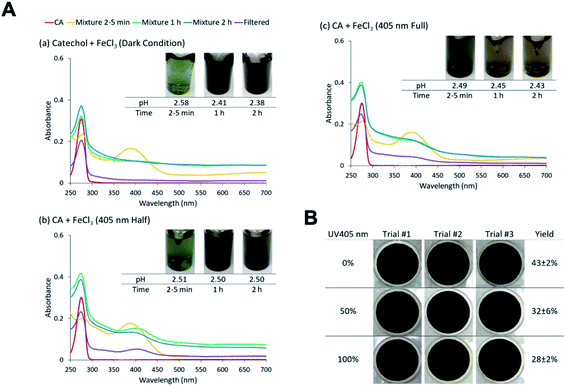 |
| | Fig. 14 (A) Effect of 405 nm irradiation on particle formation of CA and Fe(III) at different levels of UV LED intensities (0%, 50%, and 100%). Different colors of traces correspond to the spectra of CA before mixing (red), 2–5 min after mixing (orange), 1 h after mixing (green), 2 h after mixing (blue), and filtered solution (purple). (B) Photographs of filters containing particles after 2 h of reaction, filtration, and drying for pyrocatechol (CA) under different intensities of 405 nm UV irradiation. The last column contains the average (n = 3) effective mass yield in percent. Reproduced from ref. 190 under Create Commons License (CC BY-NC) from the Royal Society of Chemistry, © The Author(s), 2021. | |
In summary, polycatechol and polyguaiacol formation is efficient under dark and light conditions using millimolar concentrations of Fe(III) and organic reactants, which may be attainable on surfaces of particles or in aerosol liquid water. As stated earlier, the concentrations of these reactants are lower in cloud and fog droplets, making the extrapolation of the above results not straightforward.
5.1.6 Effect of ionic strength and viscosity on polycatechol formation under acidic conditions.
A number of factors affect the rate of reactions in atmospheric cloud/fog droplets and deliquescent aerosol systems containing Fe(II)/Fe(III) species. These factors include the concentration of reactants, pH, and ionic strength (I), which are chiefly dependent on the aerosol liquid water. As stated earlier and in the following sections, the amount of aerosol liquid water in atmospheric particles is a function of temperature, RH, and chemical composition (inorganic vs. organic).237,238 The aqueous phase volume in cloud/fog droplets is about 10−1 cm3 m−3 with pH values in the range of 2–7 and I of 10−4 M, compared to ∼10−6 cm3 m−3 in deliquescent aerosols with pH values below 2 and I > 6 M depending on the source location (e.g., marine, urban, or continental).66 These values are largely controlled by the inorganic salt content of atmospheric droplets/aerosols. The organic content in atmospheric particles is characterized by a number of functional groups with the oxygen-to-carbon elemental ratio (O:C) in the range of 0.1–1.0.35 The uptake of VOCs from biogenic and anthropogenic sources, gas and particle phase oxidation reactions can produce low-volatility products leading to the mixing of organic species with inorganic salts.35
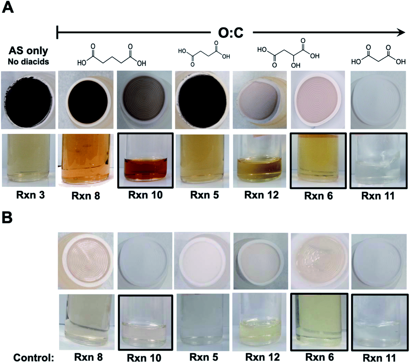
Iron-catalyzed polymerization of catechol was investigated148 under conditions characteristic of relatively viscous multicomponent aerosol systems and adsorbed water70 with high ionic strength (I = 1–12 m), acidic pH (∼2),66,237,239 and low water activity (0.6–0.97)240 for comparison with earlier studies completed under conditions typical for cloud chemistry (I = 0.01 M, pH 3–5).68,70 To vary the pH, I, and water activity, the background aqueous phase solutions were prepared by adding either ammonium sulfate (AS) or ammonium nitrate (AN), and ubiquitous C3–C5 dicarboxylic acids (malonic, malic, succinic, and glutaric acids) were detected in biomass burning aerosols163 and used in laboratory studies for investigating the liquid–liquid phase separation.35 The relative amounts of the organic (Org) and inorganic (Inorg) components were varied to achieve mass ratios reported for field aerosols, Org:Inorg = 0.2–3.5.35 These salts and diacids also competed for binding to iron, specifically the anionic species,169 forming soluble iron complexes. For example, Table 6 lists the reaction numbers and the composition of the background solutions using ammonium sulfate (AS). The concentration of chemicals was chosen to achieve an Org:Inorg (AS or AN) mass ratio between 0.5 and 2. This mass ratio range was measured in field-collected organic aerosols from the pristine Amazon Basin241 and many locations in the Northern Hemisphere.242,243 The diacids chosen for this study have an O:C molar ratio greater than or equal to 0.8. Previous work on aerosol systems containing organics with this molar ratio range showed no liquid–liquid phase separation as a function of the Org:AS mass ratio range used here.244 Instead, deliquescence (D) and efflorescence (E) were observed in these systems with DRH and ERH ranging from 45–80 and 10–35%, respectively.244 The calculated water activity in the solutions in Table 6 ranges from 0.81 to 0.99 and that using AN ranges from 0.68 to 0.99, hence covering a relatively wide range of aerosol liquid water.
Table 6 Chemical composition and physical properties of background solutions for the reaction between iron chloride and catechol using ammonium sulfate (AS) as salt. Reproduced from ref. 148 with permission from the American Chemical Society, © 2021
| Rxn no. |
[Salt] (M) |
[Org] (M) |
Ionic strng.a (m) |
Soln. densityb (gmL−1) |
Soln. viscosityc (mPa s) |
pH |
Water activityd (%RH) |
Org:AS mass ratio |
%[Fe–CA]e |
| AS only (no added organics) |
Calculated using  , where Ci is the concentration of charged species in solution in molality (m) calculated using Visual MINTEQ182 for each solution.
Calculated from the mass of a known volume.
Measured in this study using a viscometer for low viscosity fluids. The ‘—’ indicates instrument was not accurate in measuring viscosity using water-like fluids around 1 mPa s.
Calculated using E-AIM, Model IV, aqueous solutions.
Calculated using Visual MINTEQ for each solution relative to total Fe(III) aqueous species in solution. Abbreviations are: Rxn = reaction, AS = ammonium sulfate, Org = organic compound, SA = succinic acid, MA = malic acid, GA = glutaric acid, and Mal = malonic acid. M1–3 refer to the number of organic compounds in the solution per the terminology used by Marcolli et al.180 The concentrations are in the final solutions after mixing. All solutions contained final concentrations of 2 × 10⁻³ and 1 × 10⁻³ M of Fe(III) and catechol, respectively. The final solution volume of Rxn no. 1–8 was 20 mL and of Rxn no. 9–11 was 5 mL. The ‘*’ marks the reactions that were analyzed using UHPLC-UV-MS after filtration. , where Ci is the concentration of charged species in solution in molality (m) calculated using Visual MINTEQ182 for each solution.
Calculated from the mass of a known volume.
Measured in this study using a viscometer for low viscosity fluids. The ‘—’ indicates instrument was not accurate in measuring viscosity using water-like fluids around 1 mPa s.
Calculated using E-AIM, Model IV, aqueous solutions.
Calculated using Visual MINTEQ for each solution relative to total Fe(III) aqueous species in solution. Abbreviations are: Rxn = reaction, AS = ammonium sulfate, Org = organic compound, SA = succinic acid, MA = malic acid, GA = glutaric acid, and Mal = malonic acid. M1–3 refer to the number of organic compounds in the solution per the terminology used by Marcolli et al.180 The concentrations are in the final solutions after mixing. All solutions contained final concentrations of 2 × 10⁻³ and 1 × 10⁻³ M of Fe(III) and catechol, respectively. The final solution volume of Rxn no. 1–8 was 20 mL and of Rxn no. 9–11 was 5 mL. The ‘*’ marks the reactions that were analyzed using UHPLC-UV-MS after filtration.
|
| 1 |
0.01 |
— |
0.015 |
1.0 ± 0.1 |
— |
2.2 |
0.99 |
— |
1.2 |
| 2 |
1 |
— |
2.2 |
1.1 ± 0.1 |
— |
2.6 |
0.97 |
— |
0.33 |
| 3 |
2 |
— |
4.4 |
1.2 ± 0.1 |
— |
2.5 |
0.95 |
— |
0.12 |
|
|
M1 + AS
|
| 4 |
1 |
SA, 0.2 |
2.2 |
1.1 ± 0.1 |
— |
2.7 |
0.97 |
0.2 |
0.34 |
| 5 |
2 |
SA, 0.2 |
4.3 |
1.2 ± 0.1 |
— |
2.6 |
0.94 |
0.1 |
0.16 |
| 6* |
1 |
MA, 2 |
2.2 |
1.2 ± 0.1 |
— |
2.1 |
0.93 |
2.1 |
0 |
| 7 |
2 |
MA, 1 |
4.4 |
1.2 ± 0.1 |
— |
2.6 |
0.92 |
0.5 |
0 |
| 8 |
1 |
GA, 2 |
2.2 |
1.1 ± 0.1 |
— |
2.5 |
0.95 |
2.1 |
0.028 |
| 9 |
2 |
GA, 1 |
4.4 |
1.2 ± 0.1 |
— |
2.6 |
0.93 |
0.5 |
0.054 |
|
|
M2 + AS
|
| 10* |
2.9 |
SA, 0.17 |
5.8 |
1.2 ± 0.1 |
2445 ± 40 |
2.1 |
0.89 |
1.6 |
0.015 |
| GA, 4.4 |
| 11* |
2.6 |
SA, 0.28 |
5.4 |
1.3 ± 0.1 |
2445 ± 40 |
2.2 |
0.88 |
1.5 |
0 |
| Mal, 4.6 |
|
|
M3 + AS
|
| 12 |
4.4 |
SA, 0.4 |
7.9 |
1.3 ± 0.1 |
3014 ± 344 |
2.1 |
0.81 |
1.6 |
0 |
| MA, 4.9 |
| GA, 1.6 |
Fig. 15A shows digital photos of particles on filters and filtrate solutions from the reaction of catechol with Fe(III) as a function of O:C molar ratio in the background solutions listed in Table 6. For comparison, images for the control reactions in the absence of catechol are shown in Fig. 15B. These qualitative results clearly show that the insoluble black particles and brownish soluble reaction products originated from catechol. Also, the type of the diacid and its concentration relative to AS in the background solutions affected the particle density after 24 h of reaction time, as inferred from the color of the filters. This is because these diacids and AS can complex Fe(III) and hence compete with catechol.169 The formation of the iron catecholate complex, Fe(C6O2H4)+ (Fe–CA), is the first step in the oxidative polymerization mechanism. As the kinetics of the iron catecholate complex, Fe(C6O2H4)+ (Fe–CA), formation is 3× that of forming iron sulfate, Fe(SO4)2−, and iron malate, Fe(C4O5H4)+ (Fe–MA) (Table 3), and because similar kinetic data were not available for other diacids, the last column in Table 3 shows the percentage of Fe–CA complexes relative to other complexes in solution from thermodynamic modeling. These values were the basis for explaining the trend in particle density observed in Fig. 15.148 Despite the very low values of %Fe–CA in Rxn no. 2–12 (Table 6), polycatechol particles still formed (as judged by the color of the filters for reaction and control experiments) with apparent reduction in particle density with increasing concentrations of the diacids that strongly complex with iron (Mal > MA > GA). This trend correlated with the O:C molar ratio of these diacids (Table 2: 1.33 > 1.25 > 0.8, respectively). SA was removed from this list because it had lower solubility than other diacids, which prevented our ability to conduct experiments using concentrations 1 and 2 M. The case of Rxn no. 11 where Mal is the dominant diacid was the only one where no evidence of particle formation was observed. For Rxn no. 6, 7, and 12, the Visual MINTEQ thermodynamic model calculated a %Fe–CA to be zero, yet discoloration of filters was apparent after 24 h of reaction (Fig. 15). This discoloration is due to traces of polycatechol particles suggesting a significant reduction in the rate of particle growth under these reaction conditions.
 |
| | Fig. 15 (A) Digital photographs of filters and filtrate solutions after 24 h of selected reactions listed in Table 6 between catechol (1 × 10⁻³ M) and FeCl3 (2 × 10⁻³ M) in AS solutions. The photographs are arranged in the order of increasing O:C molar ratio of the most dominant diacids based on the structures shown. (B) The corresponding photographs for the control reactions in the absence of catechol. The black border marks the filtrate samples analyzed using UHPLC-UV-MS and ion chromatography-MS. Reproduced from ref. 148 with permission from the American Chemical Society, © 2021. | |
On the other hand, nitrate is a much weaker ligand than sulfate, hydroxide, and chloride,245 hence the calculated fraction of iron species in solution did not contain iron nitrate.148 The addition of the diacids to the AN solutions had a larger impact on the %Fe–CA than the increasing AN concentration. For example, increasing the concentration of AN from 0.01 to 12.3 M reduced the %Fe–CA from 9.5 to 2.4, and adding diacids further reduced %Fe–CA to be in the range 0–0.8 depending on the diacid (see Table S2 in ref. 148). The %Fe–CA in AN solutions were considerably higher than that employed for Rxn no. 1–3 using AS (Table 6), which ranged from 1.2–0.12. This difference had an impact on the rate of particle growth/agglomeration, as determined by DLS experiments. Fig. 16 shows the observed rate of polycatechol growth/aggregation as a function of I in different solutions using AS and AN with and without diacids. Using either AS or AN, and within the uncertainty of the measurement, these data showed that increasing I and addition of diacids reduced the initial rate of polycatechol growth/agglomeration. The addition of SA at 0.2 M concentration (200× higher than catechol) did not result in a statistically significant reduction in the rate at I = 1 and 2 m compared to the observed with no SA (using AN, right). These results suggest that under these conditions, the presence of iron succinate with AN did not interfere with the kinetics of the oxidative polymerization of catechol, which was not observed in the case of AS (Fig. 16 left). This result signifies the role that the type of the inorganic anion plays in the mechanism of polycatechol formation, which warrants further investigation.
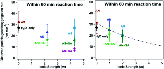 |
| | Fig. 16 Observed rate of particle growth/aggregation as a function of ionic strength (I) from the time-dependent DLS data in the first 60 min reaction between catechol (1 × 10⁻³ M) and FeCl3 (2 × 10⁻³ M) in (left) AS solutions used in different background solutions listed in Table 6, and (right) AN solution of varying compositions as per Table S2 in ref. 148. The line through the data is an exponential decay fit, y = a + be−cx, with a = 0.5 nm min−1, b = 31 nm min−1, and c = 0.2 m−1. DLS data with error bars represent ±1σ. Reproduced from ref. 148 with permission from the American Chemical Society, © 2021. | |
The reduction in the polycatechol growth/aggregation rate in solutions with high I and levels of diacids allowed for the detection of oligomers that were not observed earlier. Rxn no. 6, 10, and 11 in Table 6 were selected for mass spectrometric analysis because their filtrate solutions shown in Fig. 15 highlight the effect of dicarboxylic acids on the optical properties of the products. The retention times, m/z values, and general elemental formula of labeled chromatographic peaks in Fig. 17 are provided in Table 7. The suggested structures of the molecules with the elemental formula in Table 7 are shown in Scheme 2. The formation of the organonitrogen compound, C12H7O3N, assigned to peak 4 was confirmed using (15NH4)2SO4 and HR-MS(+) detected at m/z+ 214.0501, which is only 1.1015 ppm apart from that at m/z+ 214.0499 for C12H8O3N+. Such organonitrogen molecule was not recognized in earlier studies but is now available for further evaluation in new laboratory studies and field sampling, where it can play a role as a reactive intermediate. Hence, metal-catalyzed reactions driven by dissolved oxygen that lead to the formation of NOC in particles are potentially important pathways in systems containing ammonium and transition metals, which warrant further investigation.
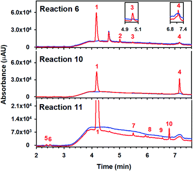 |
| | Fig. 17 UHPLC-UV chromatogram (λ = 210 nm) for (red lines) Rxn no. 6 (top), 10 (center), and 11 (bottom) after 24 h of reaction between catechol (1 × 10⁻³ M) and FeCl3 (2 × 10⁻³ M) in AS solutions, as listed in Table 6. The blue lines correspond to the respective control solutions without catechol. Except catechol (peak 1), all other labeled peaks correspond to products described in the text. Reproduced from ref. 148 with permission from the American Chemical Society, © 2021. | |
Table 7 Retention time (r.t.) for chromatographic peaks in Fig. 17 with m/z values and molecular formula in the negative and positive ion modes. See Scheme 2 for suggested structural formulae. ND = not detected. Reproduced from ref. 148 with permission from the American Chemical Society, © 2021
| Peak# |
r.t. (min) |
m/z− |
m/z+ |
Molecular formula |
| Parent |
Fragment |
Parent |
Adduct |
| 1 |
4.17 |
109.10 |
|
|
128.15 (M + NH4+) |
C6H6O2 |
| 2 |
5.02 |
207.20 |
|
|
|
C11H12O4 |
| 3 |
5.48 |
ND |
|
453.29 |
470.32 (M + NH4+) |
C18H12O14 |
| 4 |
7.16 |
212.18 |
173.19 |
214.20 |
|
C12H7O3N |
| 5 |
2.37 |
167.14 |
149.12 |
|
|
C8H8O4 |
| 6 |
2.49 |
167.10 |
123.09 |
|
|
C7H4O5 |
| 7 |
5.49 |
217.20 |
|
|
471.48 (2M + 2NH4+–H+) |
C12H10O4 |
| 8 |
6.03 |
315.25 |
|
|
334.30 (M + NH4+) |
C16H12O7 |
| 9 |
6.54 |
249.20 |
|
251.21 |
|
C12H10O6 |
| 10 |
6.79 |
365.27 |
|
|
384.31 (M + NH4+) |
C16H14O10 |
5.2 Dicarboxylic acid precursors
Unlike most dicarboxylic acids that form strong soluble complexes with iron such as oxalic and succinic acids, the reaction of unsaturated C4–C6 dicarboxylic acids detected in aged secondary organic aerosols3,164 – with Fe(III) under acidic conditions led to the efficient formation of insoluble and colored polymeric compounds, even in the presence of competing ligands such as sulfate and oxalate. Tran et al.69 showed that fumaric and muconic acids react with FeCl3 at pH 3 forming orange colored organometallic polymers, Fe-polyfumarate and Fe-polymuconate. Fig. 18 shows the photographs of reaction solutions and filters. The mass yields were found to be ∼84 ± 6% using fumarate and 52 ± 6% using muconate at pH 5 after overnight reaction. These yield values are relative to the initial concentration of the organics (2.1 mM) in control experiments at pH 5. Scheme 4 shows the proposed structures of these organometallic polymers based on the dry particle characterization using ATR-FTIR spectroscopy, TGA, transmission electron microscopy (TEM) with diffraction, scanning transmission electron microscopy-energy dispersive X-ray spectroscopy (STEM-EDS) for elemental mapping, electron energy loss spectroscopy (EELS) for oxygen K-edge, and XPS for iron oxidation state. The presence of excess oxalate in solution was found to suppress the formation of Fe-polyfumarate and Fe-polymuconate particle formation, whereas excess sulfate had no effect.68 Polymerization reactions efficiently take place in the presence of sulfate in solution producing particles with iron-coordinated and/or pore-trapped sulfate groups. When soluble iron was the limiting reagent, the insoluble product mass was reduced, highlighting the central role of excess iron in catalyzing particle formation in solution.
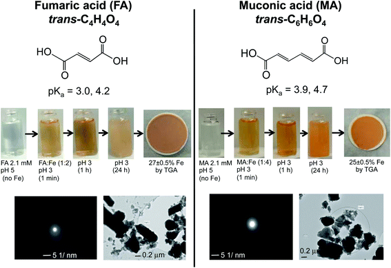 |
| | Fig. 18 Dark reaction of fumaric acid (FA, panels on the left) and muconic acid (MA, panels on the right) with FeCl3 at pH 3: (top) chemical structure and pKa values of FA and MA; (middle) digital images of the 1:2 organic reactant/Fe molar ratio of unfiltered solutions as a function of time and particles on filters after 24 h of reaction time; and (bottom) TEM images with diffraction of dry Fe-polyfumarate and Fe-polymuconate particles. Reproduced from ref. 69 with permission from the American Chemical Society, © 2021. | |
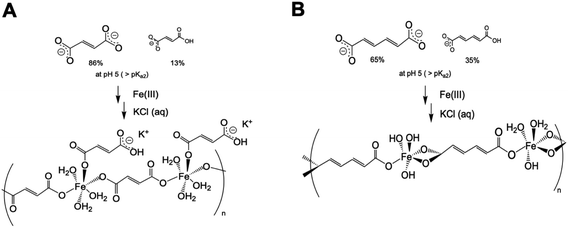 |
| | Scheme 4 Diagrams for the formation of (a) Fe-polyfumarate, and (b) Fe-polymuconate based on structural elucidation of the organometallic polymers in ref. 69. The percentages show the fraction of species in solution based on the pKa values of fumaric and muconic acids, respectively. | |
The insoluble particles were found to be amorphous, contain iron in the oxidation state between 2+ and 3+, and can form using reaction solutions at 21-fold lower organic reactant concentrations than those used in Fig. 18. These particles are responsible for the UV absorbance of unfiltered reaction solutions at 370 nm, which was assigned to the π–π* transitions in CC groups of Fe-polyfumarate and Fe-polymuconate backbone structures. The UV absorbance spectra were converted to the mass-normalized absorption coefficient (MCA) for comparison with those recorded for other BrC materials, as discussed in the following sections. For comparison, OH or ozone oxidation of FA and MA would instead produce water-soluble products that do not absorb visible light.246 Hence, the iron-catalyzed polymerization described here opens up unique pathways for processing these diacids.
Using 25–50 μM concentrations of organic diacids, the DLS experiments aimed at monitoring the particle growth in real time showed that polydispersed particles formed quickly and grew to >100 nm in hydrodynamic size after half an hour of reaction.68 The growth rate of these particles appears to depend on the final organic reactant:Fe molar ratio and pH. Within the variability of the DLS results in Fig. 19a and b, it is clear that sulfate has no significant effect on the kinetics of particle growth/agglomeration relative to the control. The addition of oxalate, on the other hand, appeared to initially produce relatively larger particles that grow to micron-size particles at a faster rate than when sulfate is added or in the control case. The product masses under these reaction conditions with oxalate and sulfate in solution resulted in values close to the control value (see Fig. 2 in ref. 68). Hence, it was concluded that the initial solution nucleation is retarded by oxalate, which produces fewer particles. In conclusion, Fe-polyfumarate and Fe-polymuconate efficiently form over a wide range of atmospherically relevant conditions. The iron centers in the amorphous structures of Fe-polyfumarate and Fe-polymuconate could act as catalysts for the dark and photochemical production of reactive oxygen species (ROS)77 such as OH and H2O2, adsorption of oxyanions such as sulfate, and reduction of NOx in the presence of ammonia. The low solubility of these particles makes them uniquely different from the much better known oligomeric compounds formed during VOC oxidation, which are commonly water soluble.247 These chemical processes will depend on the amount of ‘adsorbed water’ and aerosol liquid water. Similar to polycatechol and polyguiacol,70 and as presented in the following section on the optical properties and morphology, the presence of polymeric products in atmospheric aerosol particles would affect their absorption and scattering properties, and the high hydrophobicity of Fe-polyfumarate and Fe-polymuconate would drive their enrichment at surfaces of aerosol particles with direct consequences on their (likely poor) ability to act as clouds and ice condensation nuclei.248,249
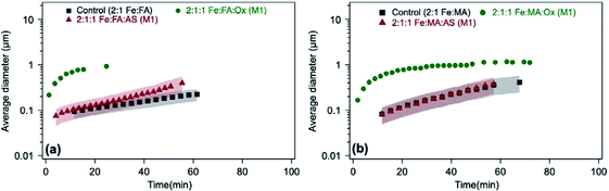 |
| | Fig. 19 Effect of adding oxalate (Ox) and ammonium sulfate (AS) on particle size from time-dependent DLS measurements during the dark aqueous phase reaction of (a) fumarate (50 μM, FA) and (b) muconate (25 μM, MA). This molar ratio results in the maximum product mass per data shown in Fig. 1. ‘M1’ stands for method 1, where organic reagents were mixed first with AS or Ox, then the reaction time started when Fe was added. ‘M2’ stands for method 2, where AS or Ox were reacted first with Fe for 2 h, then the reaction time started when the organic reagent was added. The shaded areas represent the standard deviation of three trials. Unshaded data represent the average of two trials, with a standard deviation the size of the marker width (15%). Reproduced from ref. 68 with permission from the American Chemical Society, © 2021. | |
5.3. Reactivity of BBOA aqueous extracts with iron
Reactions of BBOA aqueous extracts with Fe(III) were examined to check whether this chemistry can occur in realistic atmospheric samples.190 In these experiments, dried pine needles were burned and the resulting BBOA particles were sampled during different burning stages on Fluoropore PTFE membrane filters. Each filter was then extracted using 10 mM KCl solution at pH 3 by shaking the solution for 1 h. As not all BBOA material could be extracted using this method, the mass concentration of BBOA compounds (Cmass) in the extract was estimated using UV-vis spectroscopy where the base 10 absorbance (A) is measured in a cuvette path length (l) with a typical value of mass absorption coefficient (MAC)250 at 365 nm equal to ∼1 m2 g−1 according to eqn (25):| |  | (25) |
The molar concentration of BBOA compounds in the extract was estimated assuming an average molecular weight of 200 g mol−1. Fig. 20 shows the UV-Vis spectra of the reaction solutions of BBOA and FeCl3 at pH 3 under dark conditions and the filter after 2 h of reaction. These data show that the particle density from iron chemistry varied depending on the amount of smoldering combustion that occurred while BBOA samples were collected. Pine #1 was taken at the start of the burning when conditions could be characterized as flaming. In this case, it is very likely that the BBOA did not contain sufficient quantities of reactive catechol or guaiacol derivatives, or it contained compounds with stronger affinity to Fe(III) preventing it from particle-forming reactions such as nitrated aromatics,251,252 Pine #2 was collected later in the burning process, when at least half of the fuel burned. Upon mixing with Fe(III), the changes in the UV vis spectra and the pattern of color change of the reaction with FeCl3 were similar to those of the reaction of 4-MC and FeCl3. Given these observations and the lack of particles on the filter after 2 h of reaction, it was inferred that BBOA compounds produced during this burning stage may form complexes, but they do not partake in the subsequent polymerization over relatively short reaction times, i.e., 2 h. In the case of Pine #3, BBOA was collected after the fire was extinguished by placing a lid on the container where burning took place. This resulted in purely smoldering conditions, expected to emit lignin pyrolysis and distillation products.253 The UV-Vis spectrum for reaction solutions of Pine #3 with Fe(III) had a notable decrease over time at 480 nm that matched that of the reaction of 4-HC and FeCl3. Also, the particle mass yield was found to be 53% after 2 h of reaction with Fe(III). Therefore, it appears that BBOA produced during smoldering conditions contain hydroxylated aromatics such as 4-HC. In conclusion, the behavior of three different samples of BBOA contrasts with the highly reproducible results of experiments in which individual catechol derivatives were mixed with Fe(III), suggesting the need for further investigation of how burning conditions and fuel types affect the BBOA chemical composition and the composition of its aqueous phase extracts.
 |
| | Fig. 20 UV-Vis absorption spectra of mixture of excess Fe(III) and BBOA extracts. Different colors of traces correspond to the spectra of BBOA before mixing (red), 2 min after mixing (orange), 30 min after mixing (green), 1 h after mixing (light blue), 2 h after mixing (dark blue), and filtered solution (purple). Reproduced from ref. 190 under Create Commons License (CC BY-NC) from the Royal Society of Chemistry, © The Author(s), 2021. | |
6. Atmospheric impact of particles from iron chemistry
6.1. Dust dissolution and reactivity
The length of time mineral dust particles spend either as a wet aerosol or in cloud droplets will affect the amount of soluble iron due to aging during long range transport. The uptake of acids within clouds can also enhance iron dissolution in the droplets or in the residual aerosol formed after droplet evaporation. The chemistry described above used FeCl3 as a source of dissolved iron in aqueous phase reactions to simulate the reactivity in aged iron-containing mineral dust particles. To simulate acid-driven dissolution of freshly emitted dust and its reactivity with catechol, two types of experiments were conducted, one with hematite70 and one with Arizona Test Dust (AZTD).206Fig. 21 shows the digital images of hematite slurry following 10 days of mixing at pH 1. Also shown are images of the filtrates before and after the addition of catechol and guaiacol, in addition to the filters after 1 h of reaction. The changes observed in the color of the solutions before filtration and the presence of the polycatechol and polyguaiacol particles on the filters clearly highlight that the same chemistry takes place as that observed using FeCl3.
 |
| | Fig. 21 Formation of polycatechol and polyguaiacol from reaction with dissolved iron from acid-promoted hematite dissolution. Reproduced from ref. 70 with permission from the American Chemical Society, © 2015. | |
Using AZTD, Link et al.206 studied its reaction with dissolved catechol as functions of time and pH in the dark. The left and right panels of Fig. 22 show photographs of AZTD control (C, no catechol added) and reaction (R, with catechol) slurries over a 14 day period and that of the dry particles after filtration. Photographs of the AZTD slurries in Fig. 21 showed little change in color over the 14 d reaction time. However, the color of the particles on the filters from the reaction vials appeared darker compared to that from the control vials with no catechol. Similar studies were conducted using hematite nanoparticles under acidic pH where progressive darkening in the color of the slurry containing catechol with time was observed (see ESI in ref. 206). The darker color of the dried filters obtained after 14 d of simulated acid processing suggests that the adsorption of catechol to iron-containing materials slowly changes the surface chemical composition of the particles. Fig. 23 shows the scanning transmission electron microscopy (STEM) images of AZTD particles with catechol (top) and unreacted (bottom) following nearly two weeks of reaction at pH 1. The STEM images were coupled with energy dispersive X-ray spectroscopy (EDS) elemental mapping to show the distribution of carbon, oxygen and iron in the samples. The iron signals are concentrated in some areas where brighter areas correspond to higher relative amounts than dimmer areas. The carbon signals in Fig. 23a for particles reacted with catechol are not uniformly distributed across the image with some areas having larger amounts of detected carbon than the others. The C atomic% is higher for AZTD-Cat at 4.5% compared to undetectable for the control AZTD (no catechol in Fig. 23b). Other STEM images in ref. 206 showed that there is some co-localization of the iron and carbon signals, suggesting that the iron content in the dust particles might be anchoring the polymeric network of polycatechol, which upon formation, might encapsulate the dust particle.
 |
| | Fig. 22 Digital photographs of control (C, left) and reaction (R, right) vials containing AZTD as a function of pH and simulated atmospheric aging time. The pH values shown in the label of each vial refers to the starting pH of the slurry. At the end of day 14, the slurries were filtered and the corresponding filters are shown below each vial. The concentration of DFe in the filtrates of C-pH 1, R-pH 1, and R-pH 3 were 9.5, 12.2, and 2.3 mg L−1, respectively. Values of DFe for the other filtrate solutions were below the detection limit of the instrument (0.25 mg L−1). Reproduced from ref. 206 with permission from the American Chemical Society, © 2020. | |
 |
| | Fig. 23 Representative STEM images and EDS elemental mapping of AZTD particles with (a) polycatechol (AZTD-Cat) and (b) control (AZTD only, no catechol in solution). Slurries used for the images are shown in Fig. S3 in the ESI.† The images labeled C, O, and Fe represent the elemental maps for the corresponding atoms. In (b), no carbon signal was detected in the EDS spectrum, hence no carbon map was generated. Reproduced from ref. 206 with permission from the American Chemical Society, © 2020. | |
In the soil chemistry literature, catechol was found to undergo catalytic abiotic oxidation on the surfaces of iron and manganese oxides at basic pH (pH > 8). Scheme 5 shows a three-step mechanism for the formation of polycatechol proposed by Colarieti et al.254 Steps 1 and 2 are heterogeneous reactions, which involve the partial oxidation of catechol due to an electron transfer to surface iron and the release of Fe(II) to solution. The reduced Fe(II) species in solution further complex with catechol, which then undergoes homogeneous oxidation, step 3, in the presence of dissolved oxygen. This reaction step involves cycling between Fe(II) and Fe(III) species and the production of reactive oxygen species, H2O2 and OH radicals, as intermediates.217 Under acidic conditions relevant to atmospheric aerosol pH, the same chemistry takes place albeit over days of reaction time. Although the reaction kinetics with AZTD and HEM particles are slower under acidic relative to basic pH according to the qualitative assessment of the filter images in Fig. 22, polycatechol formation changes the optical properties of the dust and hematite particles (discussed in detail below). In summary, the change in the chemical composition of iron-containing particles driven by oxidative polymerization of catechol changes the optical properties, mixing state and morphology of the particles. The next few sections elaborate on the latter topics and their impact on the hygroscopic properties of atmospheric particles.
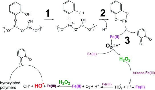 |
| | Scheme 5 A three-step mechanism for abiotic oxidative polymerization of catechol on the surface of iron oxide proposed by Colarieti et al.254 and Larson and Hufnal Jr217 The different colors are used to highlight the oxidation state of the iron in the respective step. The larger size of OH and H2O2 is used to highlight the reactive oxygen species generated in the reaction. Reproduced from ref. 206 with permission from the American Chemical Society, © 2020. | |
6.2. Mixing states and morphology
The complex chemical composition of atmospheric aerosols influences their physical properties such as the morphology and the mixing state. Aerosol morphology is a general term that reflects the apparent shape, size, and topology of particles from optical and electron microscopy images. Examples of morphology include homogeneous, phase-separated core–shell and partially engulfed.255–257 The mixing state refers to the chemical speciation and physical properties of each particle.27,31,258,259 Often the mixing state is described in terms of external and internal mixtures to refer to the number of chemical species per particle in an aerosol population. Freshly emitted particles are more externally mixed, whose atmospheric aging leads to internal mixing. Experimental measurements of the physical and chemical properties provide information on their distribution within the particle population of an aerosol. Riemer et al.31 and Laskin et al.32 reviewed the literature on the techniques used to obtain information on aerosols' mixing state, their advantages and limitations. Using some of these techniques, You et al.,35 Li et al.,260 and Song et al.257 identified mixing states beyond homogeneous-like particles that include dumb-bell, core shell and organic matter-coating, as shown in Fig. 24. These morphologies and mixing states depend on the particle size, are not static and tend to evolve over time due to multiphase aging processes in the atmosphere including the variation in the relative humidity that can lead to liquid–liquid phase separation and other phase transitions.35,257
 |
| | Fig. 24 Schematic of major atmospheric aerosol morphology and mixing states proposed by You et al.,35 Li et al.260 and Song et al.257 | |
In order to explore the mixing state and morphological changes to aqueous droplets containing organics and iron, the reaction between catechol, guaiacol, fumaric acid and Fe(III) in a micrometre-sized aqueous droplets was monitored in situ and in real time under a constant flow of humid air (∼96–100% RH) using an optical spectroscopy setup used for monitoring liquid–liquid phase separation in aqueous phase droplets at the University of British Columbia.35Fig. 25 shows images of these droplets at the beginning of the reaction for comparison with those collected after the reaction proceeded for the times specified. These images indicate that polycatechol and polyguaiacol form as ‘inclusions’ in the aqueous droplets, whereas Fe-polyfumarate forms a polymeric network at the air/aqueous interface. An animation movie in the ESI† shows the movement of this polymer at the surface of the droplet, while flowing humid air suggests a preference for the core–shell morphology. These results highlight changes to the droplet morphology, mixing state, and chemical composition due to the formation of the insoluble products from iron chemistry. These changes would have consequences on the bulk and surface chemistry of the droplets.
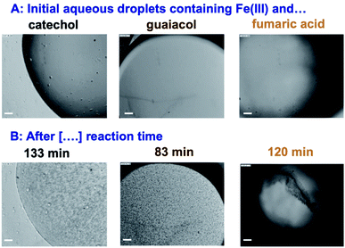 |
| | Fig. 25 Optical images of aqueous droplets showing the formation of polycatechol (left), polyguaiacol (middle) and Fe-polyfumarate (right). Left and middle images were taken from the bottom of the droplet, and the right image was taken from the top of the droplet. Reaction final concentrations were 5 mM organic precursor and 10 mM FeCl3(aq). Each droplet, of 2 μL, was ‘sandwiched’ between two slides with no flow of humid air over the droplet. After acquiring the initial images shown in the top panel, the reaction took place in the dark, with slides placed in the condition flow cell on the bench. Then, the flow cell was transferred to the microscope to collect the images during the flow of humid air at ∼ 100% RH at the specified reaction time in the lower panel. The scale bar = 0.1 mm. Unpublished results in collaboration with Professor Allan Bertram and graduate student Yuanzhou Huang at the University of British Columbia (2019). | |
6.3. Optical properties
The term aerosol optical properties refer to optical parameters that quantify aerosols' ability to scatter and absorb shortwave and longwave radiation through the imaginary (k) and real (n) parts of the particle refractive index, m = n − ik. Both components contribute to the extinction coefficient of the material of interest and vary with the wavelength, which for atmospheric aerosol particles, ranges from the near-UV to the IR part of the electromagnetic spectrum.261 As outlined in the review article by Laskin et al.,33 the measurements of optical properties will vary depending on the sample being analyzed: bulk solid aerosol materials as thin films, bulk liquid aerosol extracts, air containing aerosol particles, and aerosol-loaded filters. The refractive index of scattering particles is used in Mie theory calculations along with the size distribution to compare the calculated phase function and linear polarization for light scattering with experimental ones.262 Mie theory was derived for spherical particles and hence is limited in predicting particle scattering from non-spherical and irregularly shaped particles, as illustrated in the case of mineral dust and its components.263 These parameters are used in climate models for the calculation of the radiative forcing due to aerosol–radiation interactions (RFari).1 The values of RFari clearly show a variation depending on the chemical properties. These properties are not static and change during the lifetime of the aerosol particles.
Fig. 26 shows a graphical representation of the absorption and scattering optical parameters, namely k, mass absorption coefficient (MAC), and single scattering albedo (SSA) for three aerosol types with dominant light absorption properties as it results in positive RFari and hence have direct climate relevance,264 namely mineral dust, black carbon (BC) and brown carbon (BrC). Conceptually, the net shortwave aerosol absorption, usually quantified through the absorbing aerosol optical depth (AAOD), can therefore be thought of as the sum of the contributions of the above three separate species, integrated over the atmospheric column.264 Modeling AAOD is challenging and hence model validation, because the observed aerosol mixing state makes clear distinctions between separate aerosol types hard.258,264 The SSA values range from 0 to 1 (purely scattering). Aerosols that have SSA values below ∼0.85–0.9 indicate the absorption of solar radiation, hence they have a net positive RF.265
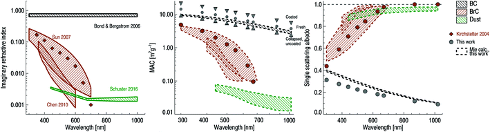 |
| | Fig. 26 Physical parameters used in modeling aerosol absorption: wavelength dependence of the imaginary refractive index (left), MAC (middle), and SSA (right). The term ‘this work’ refers to ref. 264. Reproduced from ref. 264 under Create Commons License (CC BY-NC-ND 4.0) from Springer, © The Author(s), 2018. | |
6.3.1 Mineral dust.
Mineral dust in the atmosphere is the most abundant atmospheric aerosol by mass in most global aerosol models;266,267 as a result, its absorption of solar radiation can dominate that of BC and BrC in some regions and seasons.268,269 Because climate forcing is highly sensitive to the optical properties of dust particles,270 dust radiative forcing can be positive (heating) or negative (cooling) depending on the values of key variables that include the height of the dust layer, particle size and aerosol optical depth (AOD).103 Although dust particles weakly absorb visible radiation (single scattering albedo (SSA) of dust particles is typically in excess of 0.95 at the peak of the solar spectrum271,272), the SSA value depends on the particle size and mineralogy (particularly, the hematite and goethite contents). Scanza et al.273 reported the simulation of dust radiative forcing as a function of both the mineral composition and size on the global scale, using mineral soil maps for estimating emissions. Previous field measurements showed that volatiles efficiently transfer from accumulation mode particles onto dust particles in Asian outflows,274 thus creating an environment for the possible reactions between volatiles and dust surfaces. Light-absorbing inclusions on dust have a strong effect on its optical properties, for example, internal mixing of dust particles with strongly light-absorbing black carbon has been shown to decrease the SSA for a smaller particle size.275
Al-Abadleh and co-workers reported on a chemical process that made dust more light absorbing.206 Using AZTD and hematite nanoparticles as laboratory standards and proxies for hematite-rich natural dust, respectively, they showed that reactions with catechol over 14 days of simulated acidic atmospheric aging (pH 1 and 3) lead to the formation of black polycatechol, increasing the ability of dust and hematite to absorb light over a wide range of wavelengths given its dark color. This simulated aging process was in contrast with the behavior of oxalate and sulfate that form complexes with iron sites, promoting the dissolution of iron minerals in dust. Hence, this aging chemistry may change the radiative forcing of dust aerosol from negative to positive, similar to that of black carbon. Mixing with pollution emissions during mineral dust transport is also recognized to alter the optical properties of dust.276–278 Bi et al.277 quantified the optical parameters of pure and transported anthropogenic dust over East and Central Asia for improving the accuracy of remote sensing applications and global climate models.
6.3.2 Black carbon (BC or soot).
Black carbon (BC) or soot is the most abundant light absorbing carbonaceous aerosol type, which results from the combustion of fossil fuels and biofuels. Within the current uncertainty, BC has a net positive radiative force second only to CO2.279,280 Bond and Bergstrom261 reviewed the literature on the relationship between the structure of BC and its optical parameters to be used in models. Flame-generated BC contains sp3 bonds (as in diamond) and sp2 bonds with loosely held valence electrons in p-orbitals (as in graphite) in addition to hydrogen and oxygen. Bond and Bergstrom261 suggested a narrow range of refractive indices, as highlighted in Fig. 26 (left), and a mass-normalized absorption cross section of 7.5 ± 1.2 m2 g−1 at 550 nm for uncoated particles (Fig. 26 (middle)).
Freshly emitted BC has a ‘fractal’ structure, where nanometer size particles form conglomerates. This material absorbs electromagnetic radiation across a broad spectrum because the energy levels of the loosely held electrons are closely spaced. As highlighted above, BC can be externally or internally mixed within an aerosol population, hence affecting the overall morphology of particles. Terms that highlight the morphological changes of BC particles during atmospheric aging include ‘encapsulated’, ‘inclusions’, ‘collapsed uncoated’ and ‘coated’. Fig. 27 shows the changes in morphology with atmospheric aging time leading to an enhancement in MAC and direct radiative forcing (DRF) values based on the experimental evidence by Peng et al.282 MAC values for aged BC are higher than those of fresh/uncoated particles (Fig. 26 middle). In their models,283 Boucher et al.283 used average values of 11 m2 g−1 for aged BC particles and argued that converting enhancements to increased DRF is still a work in progress. These enhancements in MAC has been explained by an optical lensing effect due to the coatings. In their review, Samset et al.264 provided a summary table for enhancement in absorption (Eabs) as a function of wavelength for three different aging cases studied in the literature: ‘pure → fresh’, ‘fresh → aged’ and ‘pure → aged’, where “pure” refers to uncoated and collapsed BC, “fresh” refers to freshly emitted BC, while “aged” refers to aged BC that has become coated. Table 8 lists these Eabs values and the source studies. Zhang et al.284 correlated the Eabs values with the chemical composition from field data collected over four seasons and found that the significant wavelength-dependent Eabs increase (from 1 to 2) correlated with the aerosol photochemical aging associated with the production of highly oxidized secondary organic aerosols (SOA), especially at summertime. Other factors that contribute to the uncertainty in BC radiative forcing calculations are residence time, vertical profiles and emission inventories.264
 |
| | Fig. 27 Time-course evolution of BC aerosol composition, light absorption (where EMAC-BC is the enhancement because of coatings relative to fresh/uncoated particles), and associated climate effects (as DRF). Reproduced from ref. 281 under the Create Commons License (CC BY-NC-ND 4.0) from the National Academies of Sciences USA, © The Authors, 2016. | |
Table 8 Overview of enhancement factors from a number of studies. Reproduced from ref. 264 under Create Commons License (CC BY-NC-ND 4.0) from Springer, © The Author(s), 2018
| Reference |
E
abs,fresh
|
E
abs,aged
|
E
abs,total
|
λ (nm) |
| Pure → fresh |
Fresh → aged |
Pure → aged |
| Bond and Bergstrøm (2006)285 |
1.5 |
1.5 |
(2.3) |
|
| Cappa et al. (2012)286 |
1.06 |
1.2 |
|
532 |
| Cui et al. (2016)287 |
1.4 |
1.7 |
3 |
678 |
| Peng et al. (2016)288 |
|
|
2.4 |
532 |
| Liu et al. (2015)289 |
1.1 |
1.4 |
|
781 |
| Healy et al. (2015)290 |
1.0 |
|
|
781 |
| Nakayama et al. (2014)291 |
1.1 |
|
|
781 |
| Sinha et al. (2017)292 |
|
|
1.44 |
565 |
| Lan et al. (2013)293 |
1.07 |
|
|
532 |
| Liu et al. (2017)294 |
|
1.1–1.6 |
|
405, 532, 781 |
6.3.3 Brown carbon (BrC).
BrC structurally differs from BC resulting in strong absorption at short wavelengths (below 500 nm) with some classes of BrC showing absorption up to 600 nm.33,264,295,296Fig. 26 shows the optical parameters and the level of uncertainty associated with each parameter used in predicting the RF of BrC. Factors contributing to this relatively large variability include the structure and effects of atmospheric aging such as lensing, photobleaching and emission inventory. The molecular structure of BrC includes tar balls, HULIS and water-soluble organic carbon (WSOC) with different classes of chromophores such as aromatic carboxylic acids, nitrophenols and substituted, heterocyclic, and pure polycyclic aromatic hydrocarbons.33,264,295,297,298 Chemical processes that lead to the formation of BrC have been reviewed earlier.33,295 These structural differences result in variable polarities, volatility,299 viscosity300 and hygroscopicity,301 which affect the reactivity.
The lensing effect that increases the absorption of BrC was found to be larger in internally mixed aerosol with BC than with non-light absorbing organic carbon.295 On the other hand, in laboratory studies, photobleaching due to irradiation with UV light at 365 nm of low molecular weight BrC was found to occur faster than high molecular weight.295 Photobleaching involves photolytic and oxidation processes that break CC and C–N bonds contributing to the light absorption properties of BrC. Simulating the photobleaching of BrC aerosol under realistic conditions using sunlight as the source remains challenging. Li et al.302 conducted lab experiments on the optical and chemical transformations of biomass burning (wood) tar proxy aerosols by nitrate radicals (NO3˙) and ozone oxidation in the dark, followed by photolysis and photochemical OH reactions in simulated daytime (Fig. 28). They found that NO3˙ reactions form secondary chromophores, such as nitroaromatic compounds and organonitrates, causing an increase in MAC of the aerosols by a factor of 2–3. The subsequent OH oxidation and direct photolysis both decompose chromophores in the NO3˙-aged wood tar aerosols, thus decreasing the absorption. Studies by Fleming et al.303 showed that the photodegradation lifetime of BrC depends on the fuel type, which ranges from 3.4 ± 1 for subalpine fir to 14 ± 1 for juniper.
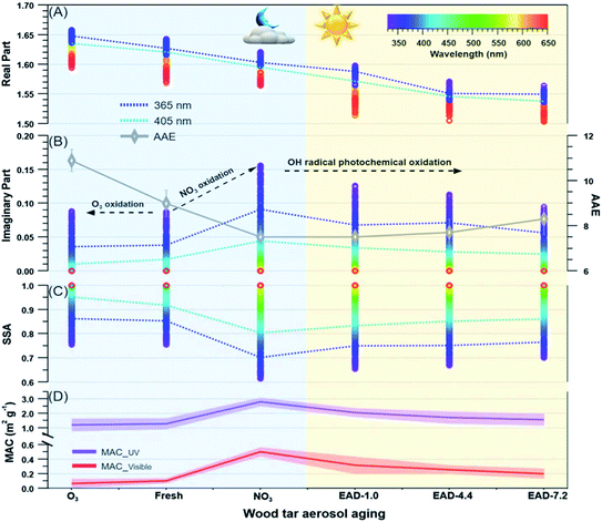 |
| | Fig. 28 Optical evolution of wood tar aerosols through various atmospheric aging processes, including O3 and NO3˙ reactions in the dark (gray area: night-time aging simulation) and photochemical transformation of NO3˙-aged wood tar aerosols (yellow area: daytime photochemical simulation). (A) Continuous wavelength-dependent complex real refractive index (RI) as a function of atmospheric transformation. (B) Continuous wavelength-dependent complex imaginary RI as a function of atmospheric evolution (left y-axis). Absorption Ångström exponent (AAE) was derived to indicate the wavelength dependence of light absorption (right y-axis). (C) Wavelength-dependent single-scattering albedo (SSA) was estimated based on retrieved refractive indices (RIs) for wood tar particles at 200 nm. (D) Changes in the wavelength-weighted mean mass absorption coefficient (MAC, m2 g−1) for wood tar aerosols via various atmospheric aging processes. Two categories are shown: near-UV absorption (330–400 nm) and visible absorption (400–550 nm). Uncertainties for each RI and SSA distributions (±0.005 for the real part, ±0.006 for the imaginary part, and ±0.013 for the SSA on average from 330 to 550 nm) are not presented for clarity. The term ‘EAD’ refers to the experimental hydroxyl radical concentration, which is equivalent to 1.0–7.2 days of ambient daytime oxidation. EAD-1.0 indicates the equivalent to 1.0 day of atmospheric aging and so forth. Reproduced from ref. 302 under Create Commons License (CC BY) from the American Chemical Society, © the Author(s), 2020. | |
In an attempt to reduce uncertainties associated with predicting RF304 of BrC, Lu et al.305 developed a method to constrain the BrC absorptivity at the emission inventory level using laboratory and field observations of POA. The main output was wavelength-dependent imaginary refractive indices (kOA) for different fuel types that include the biomass/biofuel, lignite, propane, and oil. The authors acknowledged that the effects of mixing, aging, and SOA formation need to be added to models that estimate the radiative effect of BrC.
6.3.4 BrC from iron chemistry.
Using phenolic compounds as precursors, the MAC values for the organic solvent extracts of the brown- to black-colored particles collected on the filters from the aqueous phase reactions of catechol, guaiacol, syringol, and o- and p-cresol with iron under acidic conditions were recorded by Lavi et al.211Fig. 29 (left) shows the MAC spectra for comparison with reference compounds, nigrosin, Suwannee River and Pahokee Peat Fulvic Acid (SRFA and pahokee). The solvent used in these measurement was DMSO. At 365 and 405 nm, where absorption coefficients of ambient particles are frequently measured, MAC values for guaiacol reaction products are around 1.5 × 104 cm2 g−1 in DMSO as the solvent (Fig. 29 left) and 2 × 104 cm2 g−1 in water as the solvent.70 These values are comparable to those from biomass burning aerosols (103–104 cm2 g−1)306 and in the same order of magnitude of black carbon261 (7.5 × 10⁴ m2 g−1 for uncoated soot). In the case of the guaiacol derivative, syringol, no significant absorption was measured for its reaction products with iron.
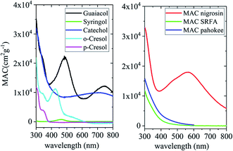 |
| | Fig. 29 Mass absorption coefficient in the UV-visible range of products formed in phenol/Fe(III) mixtures (left) and reference compounds (right). The figure and the caption were reproduced from ref. 211 with permission from the American Chemical Society, ©2017. | |
The MAC spectrum for catechol reaction products also showed relatively high values comparable with guaiacol. For comparison, Slikboer et al.70 reported the MAC spectrum for unfiltered solutions after 3 min of reaction between catechol and Fe(III) at pH 3. The intermediate peak for quinone around 390 nm70 is absent in Fig. 29 (left). The feature above 500 nm is present in both studies using DMSO and water as solvents, which resembles a similar one observed in the absorption spectrum of a mixture of polyhydroxylated benzene and C–C coupling products from the heterogeneous ozonolysis of a thin solid catechol film.207 Reaction products of phenol derivatives, o- and p-cresol, resulted in MAC spectra similar to those collected for SRFA and pahokee fulvic acid reference spectra between 300 and 500 nm, which have been used as model compounds for atmosphere BrC.33
Moreover, changes to the optical properties of diluted control and reacted AZTD slurries with catechol were reported by Link et al.206Fig. 30 shows the mass-normalized extinction coefficient (MEC) calculated in the wavelength range 300–900 nm according to eqn (26):
| |  | (26) |
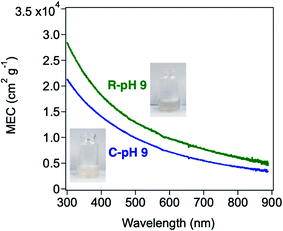 |
| | Fig. 30 Mass-normalized extinction coefficient (MEC) spectra as a function of wavelength for diluted AZTD slurries reacted with catechol at pH 9 (R-pH 9) and control at pH 9 (C-pH 9). For the controls, no catechol was added. The insets show digital photographs of the slurries used in the analysis with mass concentrations of 5.6 × 10⁻⁵ g cm−3 (R-pH 9) and 1 × 10⁻⁴ g cm−3 (C-pH 9). Reproduced from ref. 206 with permission from the American Chemical Society, © 2020. | |
MEC values for diluted AZTD slurries reacted with catechol at pH 9 (R-pH 9) and control at pH 9 (no catechol, C-pH 9). Although this high pH is not measured in LIQUID WATER, the basic pH is typically measured in the slurries of unprocessed dust due to the presence of metals that act as Lewis acid sites.123 Hence, it is likely that water adsorbed on freshly emitted dust particles would have a basic pH. The measured MEC values increased in the R-pH 9 sample at all wavelengths in agreement with the observed darkening of the particles by the reaction. This method cannot separate contributions to the increase in MEC driven by the growth of particles due to polycatechol formation, leading to increased scattering and by the deposition of light-absorbing organic material on particles leading to increased absorption. The lack of wavelength-dependent features in the MEC spectrum of the aged samples suggests that the scattering effect dominated the overall extinction.
In the case of BrC formation from aliphatic precursors, Tran et al.69 reported the MAC spectra for the reaction products of fumaric and muconic acids with Fe(III) at pH 3 as a function of reaction time (Fig. 31). As stated earlier, the dark reaction of trans-C4 and C6 unsaturated diacids with Fe(III) under acidic conditions and in the absence of any added oxidants resulted in the formation of insoluble and amorphous polymeric particles, Fe-polyfumarate and Fe-polymuconate. At 365 and 405 nm, the observed MAC values after 1 h of reaction were as high as ∼6 m2 g−1 and ∼2 m2 g−1, respectively, and higher than those shown in Fig. 29 for SRFA and pahokee fulvic acid. In the visible range, the observed MAC values drop to ∼1 m2 g−1 at 500 nm, but they still remain comparable to or higher than the typical MAC values for biomass burning aerosols. Therefore, the metal driven transformation of phenolic and aliphatic precursors detected in atmospheric aerosols with various degrees of aging is potentially an important pathway for the formation of secondary “brown carbon”.
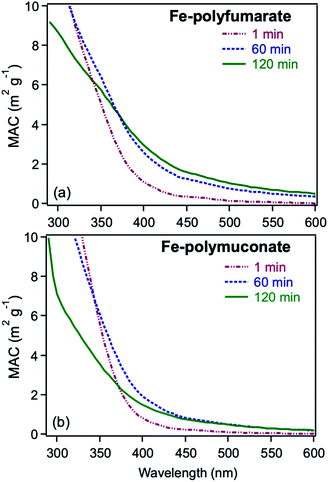 |
| | Fig. 31 Mass-normalized absorption coefficient (MAC) plot for the reaction of 0.1 mM concentration of (a) fumaric acid (FA), and (b) muconic acid (MA) with FeCl3 after 1, 60 and 120 min of dark reaction at pH 3 (unfiltered solution). The final reaction mixture contains 1:2 molar ratio organic reactant:Fe. MAC values were calculated from eqn (1) and were not corrected for the contribution from scattering by particles in solution. The figure and the caption were reproduced from ref. 69 with permission from the American Chemical Society, ©2017. | |
6.4. Hygroscopic properties
Quantifying gas-phase water uptake on atmospheric particles leads to understanding their role in air quality, climate change22 and health.23Fig. 32 shows a general schematic of the effect of RH and temperature on particle phase transitions, surface versus bulk chemistry, formation of haze, cloud condensation nuclei (CCN) and ice nuclei (IN).22 The following sections describe in detail the qualitative and quantitative aspects of aerosol liquid water on aerosol components with various solubilities for understanding the hygroscopic properties of field-collected aerosol particles. As stated above, organics from primary and secondary sources represent a major component of atmospheric aerosols, hence quantifying their hygroscopic properties is important for accurately parametrizing their climate and environmental impacts.
 |
| | Fig. 32 Interaction of water with atmospheric particles: (a) particle phase transition from solid to liquid with increasing RH; (b) particles taking up water leads to an increase in particle size and mass loading; and (c) particles participate in cloud formation by serving as CCN and IN. Reproduced from ref. 22 with permission from Oxford University Press on behalf of China Science Publishing & Media Ltd, © The Author(s), 2018. | |
6.4.1 Gas phase water uptake.
Iron-catalyzed aqueous phase reactions with catechol, guaiacol, fumaric and muconic acids produced water-insoluble and light-absorbing secondary organics particles, namely polycatechol, polyguaiacol, Fe-polyfumarate and Fe-polymuconate.69,70 Rahman and Al-Abadleh307 studied the hygroscopic properties of these particles using diffuse reflectance Fourier infrared transform spectroscopy (DRFITS) and quartz crystal microbalance (QCM) as a function of RH at 298 K. A modified 3-parameter Type II multilayer BET adsorption model described the water adsorption isotherm on the non-porous materials, polycatechol, polyguaiacol and Fe-polymuconate, whereas a Type V adsorption model (the Langmuir–Sips model) that accounts for condensation in pores was used in the case of porous Fe-polyfumarate (Fig. 33). The data revealed that organometallic polymers are more hygroscopic than organic polymers. Fig. 33 shows the water adsorption isotherms on these materials with desorption data as well. The analysis of these data shows that organometallic polymers are more hygroscopic than organic polymers and can retain more water with decreasing RH due to structural differences.
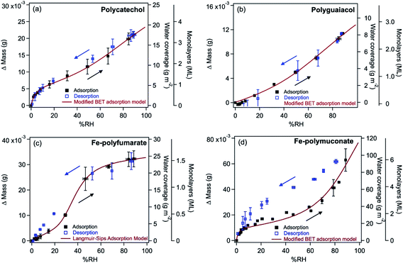 |
| | Fig. 33 Water adsorption isotherms at 298 K for (a) polycatechol, (b) polyguaiacol, (c) Fe-polyfumarate, and (d) Fe-polymuconate. The left axis shows Δmass (m), which is the change in mass due to adsorbed water, as measured using the QCM. The right axes were calculated by converting Δm to water mass (g) per surface area (m2) of the organic film deposited. The lines through the data represent least-squares best fits to the experimental data using the modified BET and the Langmuir–Sips adsorption models. The outermost right axis was obtained by dividing the water coverage in g m−2 by that at the monolayer coverage obtained from the best-fit parameters (see ref. 307 for details). Reproduced from ref. 307 under the AuthorChoice License from the American Chemical Society, © 2018. | |
6.4.2 Structure of surface water.
There are molecular level structural differences between the bulk and interfacial water on surfaces of atmospheric relevance that have consequences on the extent of water uptake, ice nucleation, ionic mobility, and chemical reactivity.77 These structural differences arise from changes to the hydrogen bonding network in the condensed phases of water that affect the fundamental vibrational modes of water.308 The use of experimental and computational tools such as infrared spectroscopy, nonlinear sum frequency generation spectroscopy, X-ray based techniques and molecular dynamics simulations provided invaluable information on the structure of interfacial water. These differences were the subject of thematic special issues of J. Phys. Chem. C309 and Phys. Chem. Chem. Phys.310
Gas phase water adsorption on the surfaces of hydrophobic organics like the insoluble polymers formed from iron-catalyzed reactions with aromatic and aliphatic precursors are two examples of insoluble aerosol components, where the uptake of water on their surfaces results in the formation of ‘adsorbed water’. Adsorbed water can take the form of either thin films or islands depending on the thermodynamic favourability of hydrogen bonding with the underlying surface. The number of hydrogen bonding donors and acceptors increase is a strong indicator for the extent of water-surface interactions. Formation of hydrogen bonding in water clusters and liquid and solid phases affects the frequencies and oscillator strengths assigned to stretching, bending and liberational modes of water.308,311–313 Also, heterogeneity (i.e., ordered vs. disordered) of the molecular environment of hydrogen bonded water can be assessed through the OH stretching band shape, which increases in broadness with increasing disorder.313 The average hydrogen bond coordination number for water molecules in bulk water is ∼3.5, which drops to 3.0 at the interface.314,315
In general, formation of hydrogen bonds in the liquid and solid bulk phases leads to the formation of broad OH stretching (ν1, ν3) and H2O bending (δ) modes and the appearance of a new combination mode. Table 9 summarizes the frequency values of water in different molecular environments. Hydrogen bonds are random and disordered and weaker in the liquid phase compared to ice, and they lead to shifting the band centre from ∼3400 to ∼3200 cm−1.316,317
Table 9 Summary of selected studies that utilized infrared spectroscopy for characterizing water in bulk phases, at interfaces and surfaces of atmospheric relevance
| Bulk phase of water |
Vibrational modes (cm−1) |
Ref. |
| Stretching |
Combination (δ + νR − νT) |
Bending (δ) |
| Symmetric (ν1) |
Asymmetric (ν3) |
|
Spectrum collected in the author's lab.
|
| H2O(g) |
3656 |
3755 |
— |
1594 |
311
|
| HDO(g) |
3622 (OH), 2723 (OD) |
3699 (OH), 2781 (OD) |
— |
1265 |
|
| H2O(l) |
3261 |
3351 |
2134 |
1639 |
323
|
| H218O(l) |
3241 |
3337 |
2130 |
1632 |
323
|
| HDO(l) |
2502 |
3404 |
2900 (2δ) |
1450 |
324
|
| D2O(l) |
2407 |
2476 |
— |
1206 |
323
|
| H2O(s) |
3289 |
3411 |
2243 |
1641 |
311
|
| Organic solid surface (powders, films) |
Adsorbed water vibrational modes (cm−1) |
Ref. |
| Stretching |
Combination (δ + νR − νT) |
Bending (δ) |
| Pollen |
3593, 3205 |
2135 |
1616 |
320
|
| Tannic acida |
3600, 3400, 3169 |
— |
1645 |
319
|
| Humic acid/goethite |
3582, 3512, 3491 |
— |
1641 |
325
|
| Polycatechol |
3580, 3020 |
— |
1628 |
307
|
| Polyguaiacol |
3580, 3170 |
1628 |
| Fe-polyfumarate |
3641, 3564, 3020 |
— |
1632 |
307
|
| Fe-polymuconate |
1628 |
| C8 and C18 self-assembled monolayers |
∼3400, ∼3180 |
— |
— |
321 and 322 |
For surface water, spectral features are often described as ‘liquid-like’ and ‘ice-like’ depending on the interface and the underlying substrate. A more accurate description refers to the strength of the hydrogen bonds: strong hydrogen bonds give rise to broad spectral features lower than 3400 cm−1 and weak hydrogen bonds between 3400 and 3500 cm−1. In the case of no hydrogen bonds, the spectral features appear sharp between 3600 and 3750 cm−1.318 In the case of hydrophobic surfaces, such as hexane and CCl4, the spectra of water show features assigned to free and bonded OH groups suggesting strong orientation effects.318 These features were also apparent on tannic acid,319 polycatechol, polyguaiacol, Fe-polyfumarate, and Fe-polymuconate307 and pollen.320 The weak and strong hydrogen bonding networks of adsorbed water on these organic powdered materials suggest cluster formation, reflecting water–water and water–organics interactions. Also, water bonding with organic functional groups acting as hydrogen bond acceptors caused shifts in their vibration modes307 and led to partial dissolution due to the formation of hydrates, as observed in the case of tannic acid.319 Water molecules in contact with organic self-assembled monolayers (SAMs) at low RH form clusters, which have fewer hydrogen bonds and gave rise to spectral components at 3200 cm−1, whereas molecules in the interior of water clusters have 3 and 4 hydrogen bonds similar to that of bulk water.321,322
6.4.3 Efficiency of cloud condensation nucleation.
Kuang et al.44 reviewed the lab and field measurements of CCN activity of SOA and highlighted the factors that affect the degree of organic aerosol hygroscopicity. These factors include the RH; water solubility; degree of atmospheric aging that affects the carbon chain length, functional groups, and oxygen to carbon (O:C) ratio; and surface tension changes due to the presence of surfactants and liquid–liquid phase separation.
To highlight the contribution of the aforementioned factors, the hygroscopic properties of lab-generated semi-solid SOA were measured as a function of RH and oxidation state through quantifying the oxygen to carbon ratio.326 The SOA were generated in a flow reactor by homogeneous nucleation and condensation following OH and/or O3 oxidation of gas-phase precursors: isoprene (C5H8), α-pinene (C10H16), and longifolene (C15H24). The hygroscopicity parameter, κ, was measured in the sub- and super-saturation RH regions using a hygroscopicity tandem differential mobility analyzer (HTDMA) and a cloud condensation nuclei counter (CCNc), yielding κHGF and κCCN, respectively. The authors calculated the ratio of κHGF to κCCN between 0 and 1 to describe a general hygroscopic behavior which is independent of absolute κ-values. κ-Ratios below 0.5 indicate the dominance of water surface adsorption, whereas those above 0.5 indicate increased solubility and higher water uptake. The phase of the SOA particles (solid, semisolid, and liquid) was quantified using an aerosol bounce instrument that yields a particle bounced fraction (BF). Particles with BF > 0 are solid or semisolid and the particles with BF = 0 behave mechanically as liquids.326 For comparison, similar experiments were conducted using solid and insoluble SiO2 spheres where water uptake occurs via surface adsorption. Fig. 34 shows a schematic that summarizes their major findings: for subsaturated conditions (RH < 100%), the water uptake of SOA with relatively low O:C (<0.6) is an adsorption-dominated process. With increasing atmospheric aging due to oxidation and increasing RH, the dissolution increases and the κ-ratio approaches 1 similar to supersaturation conditions. The authors also found that the organic precursor has an effect on the hygroscopic properties, even if the SOA O:C ratio is similar. For example, for an O:C ratio of ∼0.6, a-pinene SOA would have a κ-ratio of 0.82, whereas the κ-ratio for longifolene SOA is around 0.4.
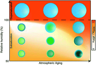 |
| | Fig. 34 Schematics of the water uptake processes of SOA particles in the atmosphere. Subsaturated swelling (κHGF) can vary dramatically with minor differences in supersaturated droplet activation (κCCN); consequently, particles can have very different direct and indirect climate effects. The background color scale indicates the ratio of these parameters under the given subsaturated and supersaturated conditions, whereas the darkness of the green color in particles denotes their atmospheric age. The contrast is the largest when adsorption is the dominant water uptake mechanism even at high RH. This is the case for low O:C SOA particles on the left. With increasing oxidation, i.e., increasing atmospheric age of the particles, the solubility increases and the dissolution RH decreases, decreasing the discrepancy between the κHGF and κCCN values. Reproduced from ref. 326 under Create Commons License (CC BY-NC-ND 4.0) from the American Geophysical Union, © The Authors, 2015. | |
Moreover, in addition to dissolution, the type of VOC precursor, and RH, Rastak et al.327 found that liquid–liquid phase separation can take place in some SOA originating from biogenic emissions with increasing RH. Fig. 35 show optical microscopy images for micrometer-scale isoprene- and α-pinene-SOA generated in the lab from photo-oxidation and ozonolysis, respectively. The SOA products were collected on a hydrophobic glass slide for collecting images at 290 K in a temperature- and RH-controlled flow cell. The presence of multiple phases is visible in the optical images. One single phase was observed over the entire RH range for isoprene-SOA, as shown in Fig. 35A, whereas for α-pinene-SOA (Fig. 35B), a single organic-rich phase is observed below 95%. Increasing the RH above 95% results in phase separation, where a water-rich phase is observed. The authors found agreement between the microscopy images and the water uptake of considerably smaller 100 nm SOA particles generated in the lab from isoprene and α-pinene. It was noted that as the O:C ratio of monoterpene-SOA changed with atmospheric aging, its hygroscopicity and CCN activity would resemble more of those of oxidized isoprene-SOA. Improved thermodynamic model predictions of κHGF were obtained when liquid–liquid phase separation was included to explore the effect of surface tension reduction by organics, as well as the coupled gas–particle partitioning of semi-volatile organic molecules and water upon RH changes.327 In the case of secondary marine aerosol consisting of sulfate, ammonium, and organic species, Mayer et al.328 found that the measured CCN activity (κapp = 0.59 ± 0.04) of the resulting secondary marine aerosol matched the values observed in previous field studies. Although these secondary particles correlate with phytoplankton biomass (i.e., chlorophyll-a concentrations), primary sea spray aerosol does not. Importantly, the authors concluded that secondary marine aerosols play a dominant role in affecting marine cloud properties.328
 |
| | Fig. 35 Optical images of micrometer scale SOA particles with increasing relative humidity. (a) Isoprene-derived SOA for mass concentrations of 70–80 μg m−3 and (b) α-pinene-derived SOA for a mass concentration of 110 μg m−3. Note that the light gray circles at the center of the particles are due to an optical effect caused by the hemispherical shape of the particles deposited on a substrate. Illustrations are shown below the images for clarity. Green: organic-rich phase. Blue: water-rich phase. The scale bar represents 20 μm. Reproduced from ref. 327 under Create Commons License (CC BY-NC-ND 4.0) from the American Geophysical Union, © The Authors, 2017. | |
6.4.4 Ice nucleation.
Understanding the role of atmospheric aerosols in cloud and ice nucleation remains at the core of minimizing uncertainties associated with the indirect effect of aerosols on the climate and the hydrological cycle. Selected recent reviews that recount the literature on the influence of aerosol chemical composition and atmospheric processes on the CCN and IN activities can be found in ref. 329–332. These reviews highlight the role of ice nucleating particles (INPs) in heterogeneous freezing, which takes place at much higher (i.e., warmer) temperatures than that required for homogeneous nucleation (<−38 °C or 235 K), and lower saturation with respect to ice (<1.5), as illustrated in Fig. 36.331Table 10 lists the brief definition of the different heterogeneous freezing processes provided by Kanji et al.330
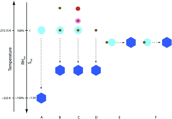 |
| | Fig. 36 Schematic overview of different ice nucleation pathways, exemplarily given as functions of temperature, relative humidity, and supersaturation with respect to ice (RHice and Sice, respectively). (A) Homogeneous ice nucleation, (B) immersion freezing, (C) deliquescence and water uptake, followed by immersion freezing, (D) deposition ice nucleation, (E) contact ice nucleation, and (F) inside-out freezing. Symbol forms and sizes are not to scale. Reprinted (adapted) from ref. 331 with permission from the American Chemical Society, © 2020. | |
Table 10 Brief definition of the heterogeneous freezing processes provided by Kanji et al.330 and Knopf et al.331
| Term |
Definition |
| Immersion freezing |
Ice nucleation initiated by an INP immersed in an aqueous solution or water droplets via activation of CCN during cloud formation. This process is suggested to be the most important for mixed phase clouds |
| Deposition ice nucleation |
Ice forms on an INP from the supersaturated gas phase (i.e., RHice > 100%). Liquid water is presumed to be absent |
| Condensation freezing |
Freezing being initiated concurrently with the initial formation of liquid on CCN at supercooled temperatures |
| Contact ice nucleation |
Ice nucleation occurs when an INP collides or comes into contact with a supercooled water or aqueous solution droplet |
| Inside-out freezing |
Freezing occurs when an INP is in contact with the liquid–air interface, establishing three interfaces (i.e., gas, solid, and liquid), under supercooled conditions |
| Pore condensation and freezing333 |
Ice formation is initiated at cirrus temperatures via the liquid phase in a two-step process involving the condensation and freezing of supercooled water inside pores |
Following decades of research, aerosols that make effective INPs have been grouped into four categories: (a) insoluble/solid inorganic particles, (b) soluble particles, (c) organics and glassy particles, and (d) nanoscale biological fragments.330 The chief examples of category (a) are mineral dust, fly and volcanic ash, K-feldspars, metal and metal oxides, and soil dust, where experiments have shown that factors such as the surface area, surface functional groups, surface defects, lattice match of surface planes with that of ice. A few highlights from selected recent studies include the following: DeMott et al.334 developed an empirical parameterization for the immersion freezing activity of natural mineral dust particles from both laboratory studies and atmospheric measurements. The dependence of immersion mode ice nucleating ability of K-feldspars (containing 85% microcline (KAlSi3O8) and 15% albite (NaAlSi3O8)) on the surface composition was investigated by Yun et al.335 to account for the effect of water-soluble inorganic solutes at low concentrations. Their study found that only K+(aq) had a positive effect (i.e., warming effect) on the ice nucleating ability of K-feldspar, while the other alkali cations, namely Li+, had no effect, and Na+, Rb+, and Cs+ had a negative effect. This trend correlated with the K/Al ratio at the surface of K-rich feldspar. Whale et al.336 investigated the immersion mode enhancement and the suppression of ice nucleation of feldspars, humic acid, quartz, amorphous silica gel, and AZTD with other alkali halides and ammonium salts. Chatre et al.337 showed that increasing the mole fraction of citric acid when AZTD is present increased the ice crystallization temperature compared to AZTD only. The effect of porosity of coal fly ash aerosol particles on their IN activity at cirrus temperatures was demonstrated by Umo et al.333 to highlight the dominance of pore condensation and freezing processes in these systems.
In the case of soluble particles such as INPs, this class contains hygroscopic salts such as ammonium sulfate and sodium chloride, which can crystallize by efflorescence. The ice nucleating ability of these salts has been extensively studied and reviewed by Kanji et al.330 Laboratory studies showed that supermicron and submicron salt particles induce heterogeneous ice nucleation via contact freezing. Pure soluble organics such as citric acid were found to promote ice nucleation near homogeneous freezing temperatures, T < −40 °C, when amorphous glass-like species form.330 Studies to date concluded that salt mixtures with organics affect the ice nucleating abilities of these systems in an unclear way because of variations in chemical composition and functional groups, phase, and morphology338 compared to single component salt systems. In their modeling study, Yun and Penner339 found that marine organic aerosol contributes to more ice formation than dust or black carbon/organic matter in mixed-phase clouds and highlighted their inclusion as natural heterogeneous ice nuclei reduced the magnitude of the total top-of-atmosphere anthropogenic aerosol force by 0.3 W m−2. The review by Knopf et al.331 examined in detail the current state of knowledge of the ice nucleating ability of organic matter in atmospheric aerosols with additional details in ref. 330 and highlighted the need for molecular level investigations to better understand the underlying mechanisms affecting organic ice nucleating abilities, particularly the structure of ice and nature of hydrogen bonding on different organic surfaces, as done for mineral clays and metal oxides.340
The impacts of solution pH and the extent of polycatechol formation on AZTD ice nucleation efficiency were investigated by Link et al.206 using the droplet freezing technique. In these experiments, microliter droplets were placed on a hydrophobic glass slide on the top of a temperature-controlled cooling stage with a cover equipped with a digital camera. The ‘frozen fraction’ was calculated from the images, which corresponds to the percentage of droplets that froze at a given temperature. The temperature that corresponds to the 50% frozen fraction is called ‘T50’ and is used as a measure of the ice nucleation efficiency of different samples. Fig. 37 shows T50 values as a function of time and pH for the control and reaction vials of AZTD (i.e., with and without catechol) over a 14 d period. The data in Fig. 37 show that polycatechol did not significantly impact ice nucleation or block ice nucleation sites on AZTD. The lack of a strong effect of polycatechol on T50 values of reacted AZTD means that polycatechol either not completely blocks the AZTD surface or is also efficient at nucleating ice. The T50 of polycatechol only was reported at −17.7 ± 0.8 °C, which is reproducibly lower than the T50 values for AZTD with polycatechol in all cases (T50 > −17 °C). This conclusion suggests that polycatechol did not completely block the AZTD surface.
 |
| | Fig. 37 Ice nucleation efficiency as gauged by T50 values as functions of time and starting pH of reaction and control AZTD slurries. Error bars in T50 represent propagated ±2σ. The figure and the caption were reproduced from ref. 206 with permission from the American Chemical Society, © 2020. | |
The data in Fig. 37 show that in the absence of catechol, increasing pH decreased the ice nucleation ability of AZTD. The shift in T50 values of 3.8 ± 1.3 and 4.7 ± 1.6 °C, respectively, due to more basic pH might be explained by the change in the protonation state of the surface of the minerals identified in AZTD. The impairment of freezing efficiency of AZTD under the basic condition can be expected, since studies341,342 have shown that the freezing efficiency of potassium-rich feldspar and quartz was suppressed under alkaline conditions, and feldspars and quartz make up a significant portion (nearly 50% in total) of the AZTD samples investigated.
7. Summary and outlook
This review recounted the current state of knowledge of iron chemistry in multicomponent atmospheric aerosol systems containing ubiquitous phenolic compounds, dicarboxylic acids, ammonium sulfate and ammonium nitrate that lead to efficient brown carbon formation in the aqueous phase. This chemistry was shown to take place using extracts of BBOA and to change the optical properties and mixing states of dust and hematite particles. Since reactive oxygen species are generated in the presence of iron, as shown in the mechanism of brown carbon formation from aromatic precursors, the atmospheric importance of these reactions can only be assessed by comparing to the HOx source strength. The laboratory studies summarized here highlight the need for additional systematic experiments that focus on the (1) effect of specific burning conditions and the nature of the fuel on the BBOA particle composition and its aqueous phase extract. This way, the extent of the reactivity of iron with organics producing BrC would be better predicted, (2) kinetics of the Fe(III)/Fe(II) cycling in reaction systems that produce BrC. This cycling of redox species can be followed by flow injection analysis and also online monitoring by continuous flow analysis,343,344 where the concentrations of Fe(II) and total Fe after the reduction of Fe(III) can be determined on the basis of the color of the reaction, (3) effect of organic compounds that do not form complexes with Fe(III) but can scavenge the ROS species that form in situ from the cycling of Fe(III)/Fe(II) in the presence of dissolved oxygen such as the OH radical.345 These organic compounds could indirectly limit the extent of the chemistry leading to colored product formation, (4) changes to the size, mixing state, and optical properties of suspended aqueous microdroplets containing soluble iron due to the gas phase uptake of semivolatile phenolic compounds, and (5) mechanisms of how soluble and insoluble products summarized here affect the aqueous phase chemistry. The results of these experiments would then be compared with similar ones conducted in a beaker or with thin films to explore the effect of micro- and nano-level reaction environments on the products.
Moreover, the research summarized in this review highlights the need to strategically design field campaigns that (1) track the processing of iron-containing particles in polluted areas or those impacted by biomass burning emissions and (2) explore the changes to iron speciation and fate upon deposition of iron containing secondary particles to the ocean surface microlayer.21 The atmospheric chemistry models need to incorporate reactions of iron with organics that lead to particle formation and not only soluble complexes. These models could also impart knowledge for planning new laboratory studies and field measurements to minimize uncertainty associated with pathways that lead to SOA and BrC formation and aging.
Author contributions
H. A. A. conceived the idea and organization of this review and fully wrote the manuscript.
Conflicts of interest
There are no conflicts to declare.
Acknowledgements
The author acknowledges contributions to experiments and data analysis from students at Laurier, the University of California Irvine (UCI), the University of British Columbia (UBC), the University of Kentucky (UKY), and the University of Maryland (UMD). Also, the author is grateful to the stimulating discussions and fruitful collaborations with professor Sergey Nizkorodov (UCI), professor Allan Bertram (UBC), professor Nicholas Meskhidze (North Carolina State University), professor Marcelo Guzman (UKY), professor Sasho Gligorovski (Chinese Academy of Science) and professor Akua Asa-Awuku (UMD). Financial support to the atmospheric chemistry research program in the author's lab was provided by Wilfrid Laurier University, Natural Science and Research Council of Canada (NSERC) Discovery, Canadian Foundation for Innovation Leaders Opportunities Fund (CFI-LOF), and the Fulbright Canada Visiting Research Chair Program at UCI.
References
-
O. Boucher, D. Randall, P. Artaxo, C. Bretherton, G. Feingold, F. Forster, V.-M. Kerminen, Y. Kondo, H. Liao, U. Lohmann, P. Rasch, S. K. Satheesh, S. Sherwood, B. Stevens and X. Y. Zhang, in Climate Change 2013: the Physical Science Basis. Contribution of Working Group I to the Fifth Assessment Report of the Intergovernmental Panel on Climate Change, ed. T. F. Stocker, D. Qin, G.-K. Plattner, M. Tignor, S. K. Allen, J. Boschung, A. Nauels, Y. Xia, V. Bex and P. M. Midgley, Cambridge University Press, Cambridge, United Kingdom and New York, NY, USA, 2013, pp. 571–657 Search PubMed.
-
J. Heintzenberg, F. Raes and S. E. Schwartz, in Atmospheric Chemistry in a Changing World - an Integration and Synthesis of a Decade of Tropospheric Chemistry Research, ed. G. Brasseur, R. G. Prinn and A. A. P. Pszenny, Springer, Berlin, 2003, pp. 125–156 Search PubMed.
-
B. J. Finlayson-Pitts and J. N. Pitts Jr, Chemistry of the Upper and Lower Atmosphere, Academic Press, New York, 2000 Search PubMed.
-
J. H. Seinfeld and S. N. Pandis, Atmospheric Chemistry and Physics: from Air Pollution to Climate Change, Wiley, New York, 2006 Search PubMed.
-
C. Tomasi and A. Lupi, in Atmospheric Aerosols: Life Cycles and Effects on Air Quality and Climate, ed. C. Tomasi, S. Fuzzi and A. Kokhanovsky, Wiley-VCH Verlag GmbH & Co., Weinheim, Germany, 2016, ch. 1, pp. 1–86 Search PubMed.
-
O. Boucher, Atmospheric Aerosols: Properties and Impacts, Springer, France, 2015 Search PubMed.
- V.-M. Kerminen, X. Chen, V. Vakkari, T. Petaja, M. Kulmala and F. Bianchi, Environ. Res. Lett., 2018, 13, 1–38 CrossRef.
- S. Philip, R. V. Martin, G. Snider, C. L. Weagle, A. van Donkelaar, M. Brauer, D. K. Henze, Z. Kilmont, C. Venkataraman, S. K. Guttikunda and Q. Zhang, Environ. Res. Lett., 2017, 12, 1–7 CrossRef.
- S. A. Weichenthal, K. G. Pollitt and P. J. Villeneuve, Environ. Health, 2013, 12, 1–8 CrossRef PubMed.
- W. Shi, T. Li, Y. Zhang, Q. Sun, C. Chen, J. Wang, J. Fang, F. Zhao, P. Du and X. Shi, Environ. Sci. Technol., 2020, 54, 16006–16016 CrossRef CAS PubMed.
- P. J. Landrigan, R. Fuller, N. J. R. Acosta, O. Adeyi, R. Arnold, N. Basu, A. B. Baldé, R. Bertollini, S. Bose-O’Reilly, J. I. Boufford, P. N. Breysse, T. Chiles, C. Mahidol, A. M. Coll-Seck, M. L. Cropper and J. Fobil,
et al.
, Lancet, 2018, 391, 462–512 CrossRef.
- M. Bruggemann, R. Xu, A. Tilgner, K. C. Kwon, A. Mutzel, H. Y. Poon, T. Otto, T. Schaefer, L. Poulain, M. N. Chan and H. Herrmann, Environ. Sci. Technol., 2020, 54, 3767–3782 CrossRef PubMed.
- Y. B. Lim, H. Kim, J. Y. Kim and B. J. Turpin, Atmos. Chem. Phys., 2016, 16, 12631–12647 CrossRef CAS.
- M. K. Shrivastava, C. D. Cappa, J. Fan, A. H. Goldstein, A. B. Guenther, J. L. Jimemez, C. Kuang, A. Laskin, S. T. Martin, N. L. Ng, T. Petaja, J. R. Pierce, P. J. Rasch, P. Roldan, J. H. Seinfeld, J. E. Shilling, J. N. SMith, J. A. Thornton, R. Volkamer, J. Wang, D. R. Worsnop, R. A. Zaveri, A. Zelenyuk and Q. Zhang, Rev. Geophys., 2017, 55, 509–559, DOI:10.1002/2016RG000540.
- M. Hallquist, J. C. Wenger, U. Baltensperger, Y. Rudich, D. Simpson, M. Claeys, J. Dommen, N. M. Donahue, C. George, A. H. Goldstein, J. F. Hamilton, H. Herrmann, T. Hoffmann, Y. Iinuma, M. Jang, M. E. Jenkin, J. L. Jimenez, A. Kiendler-Scharr, W. Maenhaut, G. McFiggans, T. F. Mentel, A. Monod, A. S. H. Prevot, J. H. Seinfeld, J. D. Surratt, R. Szmigielski and J. Wildt, Atmos. Chem. Phys., 2009, 9, 5155–5236 CrossRef CAS.
- A. L. Steiner, Acc. Chem. Res., 2020, 53, 1260–1268 CrossRef CAS PubMed.
- R. M. Hoesly, S. J. Smith, L. Feng, Z. Klimont, G. Janssens-Maenhout, T. Pitkanen, J. J. Seibert, L. Vu, R. J. Andres, R. M. Bolt, T. C. Bond, L. Dawidowski, N. Kholod, J. Kurokawa, M. Li, L. Liu, Z. Lu, M. C. P. Moura, P. R. O'Rourke and Q. Zhang, Geosci. Model Dev., 2018, 11, 369–408 CrossRef CAS.
-
D. J. Jacob, Introduction to Atmospheric Chemistry, Princeton University Press, Princeton, NJ, 1999 Search PubMed.
- M. Kanakidou, S. Myriokefalitakis and K. Tsigaridis, Environ. Res. Lett., 2018, 13, 063004 CrossRef , 063001–063022..
- N. Mahowald, Science, 2011, 334, 794–796 CrossRef CAS PubMed.
- N. Meskhidze, C. Volker, H. A. Al-Abadleh, K. Barbeau, M. Bressac, C. Buck, R. M. Bundy, P. L. Croot, Y. Feng, A. Ito, A. M. Johansen, W. M. Landing, J. Mao, S. Myriokefalitakis, D. Ohnemus, B. Pasquier and Y. Ye, Mar. Chem., 2019, 217, 103704 CrossRef CAS , 103701–103716..
- Z. Wu, J. Chen, Y. Wang, Y. Zhu, Y. Liu, B. Yao, Y. Zhang and M. Hu, Natl. Sci. Re, 2018, 5, 452–454 CrossRef CAS.
- T. V. Vu, J. M. Delagad-Saborit and R. M. Harrison, Air Qual., Atmos. Health, 2015, 8, 429–440 CrossRef CAS.
- P. H. McMurry, Atmos. Environ., 2000, 34, 1959–1999 CrossRef CAS.
-
Aerosol Measurement: Principles, Techniques and Applications, ed. P. Kulkarni, P. A. Baron and K. Willeke, Wiley, New Jersey, 2011 Search PubMed.
-
Fundamentals and Applications in Aerosol Spectroscopy, ed. R. Signorell and J. P. Reid, CRC Press, Boca Raton, 2011 Search PubMed.
- A. P. Ault and J. L. Axson, Anal. Chem., 2017, 89, 430–452 CrossRef CAS PubMed.
- M. Tang, C. K. Chan, Y. J. Li, H. Su, Q. Ma, Z. Wu, G. Zhang, Z. Wang, M. Ge, M. Hu, H. He and X. Wang, Atmos. Chem. Phys., 2019, 19, 12631–12686 CrossRef CAS.
- N. Hiranuma, S. Augustin-Bauditz, H. Bingemer, C. Budke, J. Curtius, A. Danielczok, K. Diehl, K. Dreischmeier, M. Ebert, F. Frank, N. Hoffmann, K. Kandler, A. Kiselev, T. Koop, T. Leisner, O. Mohler, B. Nillius, A. Peckhaus, D. Rose, S. Weinbruch, H. Wex, Y. Boose, P. J. DeMott, J. D. Hader, T. C. J. Hill, Z. A. Kanji, G. R. Kulkarni, E. J. T. Levin, C. S. McCluskey, M. Murakami, B. J. Murray, D. Niedermeier, M. D. Petters, D. O'Sullivan, A. Saito, G. P. Schill, T. Tajiri, M. A. Tolbert, A. Welti, T. F. Whale, T. P. Wright and K. Yamashita, Atmos. Chem. Phys., 2015, 15, 2489–2518 CrossRef CAS.
- S. Garimella, T. B. Kristensen, K. Ignatius, A. Welti, J. Voigtlander, G. R. Kulkarni, F. Sagan, G. L. Kok, J. Dorsey, L. Nichman, D. A. Rothenberg, M. Rosch, A. C. R. Kirchgabner, R. Ladkin, H. Wex, T. W. Wilson, L. A. Ladino, J. P. D. Abbatt, O. Stetzer, U. Lohmann, F. Stratmann and D. J. Cziczo, Atmos. Chem. Phys., 2016, 9, 2781–2795 CAS.
- N. Riemer, A. P. Ault, M. West, R. L. Craig and J. H. Curtis, Rev. Geophys., 2019, 57, 187–249 CrossRef.
- A. Laskin, R. C. Moffet and M. K. Gilles, Acc. Chem. Res., 2019, 52, 3419–3431 CrossRef CAS PubMed.
- A. Laskin, J. Laskin and S. A. Nizkorodov, Chem. Rev., 2015, 115, 4335–4382 CrossRef CAS PubMed.
- J. P. Reid, A. K. Bertram, D. O. Topping, A. Laskin, S. T. Martin, M. D. Petters, F. D. Pope and G. Rovelli, Nat. Commun., 2018, 9, 1–14 CrossRef CAS PubMed.
- Y. You, M. L. Smith, M. Song, S. T. Martin and A. K. Bertram, Int. Rev. Phys. Chem., 2014, 33, 43–77 Search PubMed.
- H. O. T. Pye, A. Nenes, B. Alexander, A. P. Ault, M. C. Barth, S. L. Clegg, J. L. Collett Jr, K. M. Fahey, C. J. Hennigan, H. Herrmann, M. Kanakidou, J. T. Kelly, I.-T. Ku, V. F. McNeill, N. Riemer, T. Schaefer, G. Shi, A. Tilgner, J. T. Walker, T. Wang, R. Weber, J. Xing, R. A. Zaveri and A. Zuend, Atmos. Chem. Phys., 2020, 20, 4809–4888 CrossRef CAS PubMed.
- M. A. Freedman, E.-J. E. Ott and K. E. Marak, J. Phys. Chem. A, 2019, 123, 1275–1284 CrossRef CAS PubMed.
- M. V. Johnston and D. E. Kerecman, Annu. Rev. Anal. Chem., 2019, 12, 247–274 CrossRef CAS PubMed.
-
R. M. B. O. Duarte and A. C. Duarte, in Ann. Rep. NMR Spec., ed. G. A. Webb, 2017, vol. 92, ch. 2, pp. 83–135 Search PubMed.
- S.-H. Lee and H. C. Allen, Anal. Chem., 2012, 84, 1196–1201 CrossRef CAS PubMed.
- K. M. Prather, C. D. Hatch and V. H. Grassian, Annu. Rev. Anal. Chem., 2008, 1, 485–514 CrossRef CAS PubMed.
-
P. A. Solomon, M. P. Fraser and P. Herckes, in Aerosol Measurement: Principles,
Techniques, and Applications, ed. P. Kulkarni, P. A. Baron and K. Willeke, John Wiley & Sons, Inc., Hoboken, NJ, 3rd edn, 2011, ch. 9, pp. 153–177 Search PubMed.
- G. Myhre, B. H. Samset, M. Schulz, Y. Balkanski, S. Bauer, T. K. Berntsen, H. Bian, N. Bellouin, M. Chin and T. Diehl,
et al.
, Atmos. Chem. Phys., 2013, 13, 1853–1877 CrossRef CAS.
- Y. Kuang, W. Xu, J. Tao, N. Ma, C. Zhao and M. Shao, Currrent Poll. Rep., 2020, 6, 410–424 CrossRef CAS.
- S. T. Martin, Chem. Rev., 2000, 100, 3403–3454 CrossRef CAS PubMed.
- L. J. Mauer and L. S. Taylor, Annu. Rev. Food Sci. Technol., 2010, 1, 41–63 CrossRef CAS PubMed.
- U. K. Krieger, C. Marcolli and J. P. Reid, Chem. Soc. Rev., 2012, 41, 6631–6662 RSC.
- M. Bilde, K. Barsanti, M. Booth, C. D. Cappa, N. M. Donahue, E. U. Emanuelsson, G. McFiggans, U. K. Krieger, C. Marcolli and D. O. Topping,
et al.
, Chem. Rev., 2015, 115, 4115–4156 CrossRef CAS PubMed.
- A. K. Bertram, S. T. Martin, S. J. Hanna, M. L. Smith, A. Bodsworth, Q. Chen, M. Kuwata, A. Liu, Y. You and S. R. Zorn, Atmos. Chem. Phys., 2011, 11, 10995–11006 CrossRef CAS.
- P. S. Monks, Chem. Soc. Rev., 2005, 34, 376–395 RSC.
- S. S. Brown, T. B. Ryerson, A. G. Wollny, C. A. Brock, R. Peltier, A. P. Sullivan, R. J. Weber, W. P. Dube, M. Trainer, J. F. Meagher, F. C. Fehsenfeld and A. R. Ravishankara, Science, 2006, 311, 67–80 CrossRef CAS PubMed.
- J. Kleffmann, ChemPhysChem, 2007, 8, 1137–1144 CrossRef CAS PubMed.
- R. Atkinson and J. Arey, Chem. Rev., 2003, 103, 4605 CrossRef CAS PubMed.
- H. Chen, M. E. Varner, B. Gerber and B. J. Finlayson-Pitts, J. Phys. Chem. B, 2016, 120, 1526–1536 CrossRef CAS PubMed.
- D. M. Cwiertny, M. A. Young and V. H. Grassian, Annu. Rev. Phys. Chem., 2008, 59, 27–51 CrossRef CAS PubMed.
- C. George, M. Ammann, B. D'Anna, D. J. Donaldson and S. A. Nizkorodov, Chem. Rev., 2015, 115, 4218–4258 CrossRef CAS PubMed.
- D. J. Donaldson and K. T. Valsaraj, Environ. Sci. Technol., 2010, 44, 865–873 CrossRef CAS PubMed.
- I. J. George and J. P. D. Abbatt, Nat. Chem., 2010, 2, 713–722 CrossRef CAS PubMed.
- E. Harris, B. Sinha, D. van Pinxteren, A. Tilgner, K. W. Fomba, J. Schneider, A. Roth, T. Gnauk, B. Fahlbusch, S. Mertes, T. Lee, J. Collett, S. Foley, S. Borrmann, P. Hoppe and H. Herrmann, Science, 2013, 340, 727–730 CrossRef CAS PubMed.
- Q. Chen, T. Sherwen, M. Evans and B. Alexander, Atmos. Chem. Phys., 2018, 18, 13617–13637 CrossRef CAS.
- D. J. Donaldson and V. Vaida, Chem. Rev., 2006, 103, 4717–4729 CrossRef PubMed.
-
R. Zhao, A. K. Y. Lee, C. Wang, F. Wania, J. P. S. Wong, S. Zhou and J. P. D. Abbatt, in Advances in Atmospheric Chemistry, ed. J. R. Barker, A. L. Steiner and T. J. Wallington, World Scientific, New Jersey, 2019, vol. 2, ch. 2, pp. 95–184 Search PubMed.
- J. H. Kroll and J. H. Seinfeld, Atmos. Environ., 2008, 42, 3593–3624 CrossRef CAS.
- S. M. Murphy, A. Sorooshian, J. H. Kroll, N. L. Ng, P. S. Chhabra, C. Tong, J. D. Surratt, E. Knipping, R. C. Flagan and J. H. Seinfeld, Atmos. Chem. Phys., 2007, 7, 2313–2337 CrossRef CAS.
-
N. M. Donahue, A. L. Robinson, E. R. Trump, I. Riipinen and J. H. Kroll, in Atmospheric and Aerosol Chemistry, Topics in Current Chemistry, ed. V. F. McNeill and P. Ariya, Springer, Berlin, Heidelberg, 2012, vol. 339, pp. 97–143 Search PubMed.
- H. Herrmann, T. Schaefer, A. Tilgner, S. A. Styler, C. Weller, M. Teich and T. Otto, Chem. Rev., 2015, 115, 4259–4334 CrossRef CAS PubMed.
- C. R. C. R. Hoyle, C. C. Fuchs, E. Järvinen, H. Saathoff, A. Dias, I. El Haddad, M. Gysel, S. C. Coburn, J. Tröstl, A.-K. Bernhammer, F. Bianchi, M. Breitenlechner, J. C. J. C. Corbin, J. Craven, N. M. Donahue, J. Duplissy, S. Ehrhart, C. Frege, H. Gordon, N. Höppel, M. Heinritzi, T. B. Kristensen, U. Molteni and L. Nichman,
et al.
, Atmos. Chem. Phys., 2016, 16, 1693–1712 CrossRef CAS.
- A. Al Nimer, L. Rocha, M. A. Rahman, S. A. Nizkorodov and H. A. Al-Abadleh, Environ. Sci. Technol., 2019, 53, 6708–6717 CrossRef CAS PubMed.
- A. Tran, G. William, S. Younus, N. N. Ali, S. L. Blair, S. A. Nizkorodov and H. A. Al-Abadleh, Environ. Sci. Technol., 2017, 51, 9700–9708 CrossRef CAS PubMed.
- S. Slikboer, L. Grandy, S. L. Blair, S. A. Nizkorodov, R. W. Smith and H. A. Al-Abadleh, Environ. Sci. Technol., 2015, 49, 7793–7801 CrossRef CAS PubMed.
- C. Wang, Y. D. Lei, S. Endo and F. Wania, Environ. Sci. Technol., 2014, 48, 13238–13245 CrossRef CAS PubMed.
- J. H. Seinfeld, Nat. Geosci., 2008, 1, 15–16 CrossRef CAS.
- M. Tang, D. J. Cziczo and V. H. Grassian, Chem. Rev., 2016, 116, 4205–4259 CrossRef CAS PubMed.
- B. A. Maher, J. M. Prospero, D. Mackie, D. Gaiero, P. P. Hesse and Y. Balkanski, Earth-Sci. Rev., 2010, 99, 61–97 CrossRef CAS.
- N. Mahowald, A. R. Baker, G. Bergametti, N. Brooks, R. A. Duce, T. D. Jickells, N. Kubilay, J. M. Prospero and I. Tegen, Global Biogeochem. Cycles, 2005, 19, GB4025 Search PubMed , 4021–4015..
- T. M. Conway and S. G. John, Nature, 2014, 511, 212–215 CrossRef CAS PubMed.
- H. A. Al-Abadleh, RSC Adv., 2015, 5, 45785–45811 RSC.
- C. R. Usher, A. E. Michel and V. H. Grassian, Chem. Rev., 2003, 103, 4883–4940 CrossRef CAS PubMed.
- S. R. Taylor, Geochim. Cosmochim. Acta, 1964, 28, 1273–1285 CrossRef CAS.
- P. N. Sedwick, E. r. Sholkovitz and T. M. Church, Geochem., Geophys., Geosyst., 2007, 8, Q10Q06 CrossRef.
- P. N. Sedwick, E. R. Sholkovitz and T. M. Church, Geochem., Geophys., Geosyst., 2007, 8, Q10Q06 CrossRef.
- H. Chen, A. Laskin, J. Baltrusaitis, C. A. Gorski, M. M. Scherer and V. H. Grassian, Environ. Sci. Technol., 2012, 46, 2112–2120 CrossRef CAS PubMed.
- C. Guieu, S. Bonnet, T. Wagener and M.-D. Loye-Pilot, Geophys. Res. Lett., 2005, 32, L19608, DOI:10.1029/2005GL022962.
- A. Ito, Environ. Sci. Technol. Lett., 2015, 2, 70–75 CrossRef CAS.
- A. Ito, S. Myriokefalitakis, M. Kanakidou, N. Mahowald, R. A. Scanza, D. S. Hamilton, A. R. Baker, T. D. Jickells, M. Sarin, S. Bikkina, Y. Gao, R. U. Shelley, C. S. Buck, W. M. Landing, A. R. Bowie, M. M. G. Perron, C. Guieu, N. Meskhidze, M. S. Johnson, Y. Feng, J. F. Kok, A. Nenes and R. A. Duce, Sci. Adv., 2019, 5, eaau7671 CrossRef CAS PubMed.
- R. M. Harrison, A. M. Jones, J. Gietl, J. X. Yin and D. C. Green, Environ. Sci. Technol., 2012, 46, 6523–6529 CrossRef CAS PubMed.
- M. Schulz, J. M. Prospero, A. R. Baker, F. Dentener, L. Ickes, P. S. Liss, N. Mahowald, S. Nickovic, C. P. Garcia-Pando, S. Rodriguez, M. Sarin, I. Tegen and R. A. Duce, Environ. Sci. Technol., 2012, 46, 10390–10404 CrossRef CAS PubMed.
- A. Ito and Z. Shi, Atmos. Chem. Phys., 2016, 16, 85–99 CrossRef CAS.
- M. Oakes, R. J. Weber, B. Lai, A. Russell and E. D. Ingall, Atmos. Chem. Phys., 2012, 12, 745–756 CrossRef CAS.
- A. J. Butler, M. S. Andrew and A. G. Russell, J. Geophys. Res.: Atmos., 2003, 108, SOS3-1–SOS3-11 CrossRef.
- P. Hoffmann, A. N. Dedik, J. Ensling, S. Weinbruch, S. Weber, T. Sinner, P. Gutlich and H. M. Ortner, J. Aerosol Sci., 1996, 27, 325–327 CrossRef CAS.
- A. M. Johansen, R. Siefert and M. R. Hoffmann, J. Geophys. Res.: Atmos., 2000, 105, 15277–15312 CrossRef CAS.
- W. Liu, Y. H. Wang, A. Russell and E. S. Edgerton, Atmos. Environ., 2005, 39, 4453–4470 CrossRef CAS.
- M. Oakes, N. Rastogi, B. J. Majestic, M. Shafer, J. J. Schauer, E. S. Edgerton and R. J. Weber, J. Geophys. Res.: Atmos., 2010, 115, 1–12 CrossRef.
- A. P. Ault, T. M. Peters, E. J. Sawvel, G. S. Casuccio, R. D. Willis, G. A. Norris and V. H. Grassian, Environ. Sci. Technol., 2012, 46, 4331–4339 CrossRef CAS PubMed.
- T. L. Guasco, L. A. Cuadra-Rodriguez, B. E. Pedler, A. P. Ault, D. B. Collins, D. Zhao, M. J. Kim, M. J. Ruppel, S. C. Wilson, R. S. Pomeroy, V. H. Grassian, F. Azam, T. H. Bertram and K. A. Prather, Environ. Sci. Technol., 2014, 48, 1324–1333 CrossRef CAS PubMed.
- A. P. Ault, M. J. Moore, H. Furutani and K. A. Prather, Environ. Sci. Technol., 2009, 43, 3500–3506 CrossRef CAS PubMed.
- A. P. Ault, C. J. Gaston, Y. Wang, G. Dominguez, M. H. Thiemen and K. A. Prather, Environ. Sci. Technol., 2010, 44, 1954–1961 CrossRef CAS PubMed.
- K. Deboudt, P. Flament, M. Choel, A. Gloter, S. Sobanska and C. Colliex, J. Geophys. Res.: Atmos., 2010, 115, D24207 CrossRef.
- C. Oppo, S. Bellandi, N. D. Innocenti, A. M. Stortini, G. Loglio, E. Schiavuta and R. Cini, Mar. Chem., 1999, 63, 235–253 CrossRef CAS.
- S. R. Piotrowicz, R. A. Duce, J. L. Fasching and C. P. Weisel, Mar. Chem., 1979, 7, 307–324 CrossRef CAS.
- C. P. Weisel, R. A. Duce, J. L. Fasching and R. W. Heaton, J. Geophys. Res.: Atmos., 1984, 89, 1607–1618 CrossRef.
- O. A. Choobari, P. Zawar-Reza and A. Sturman, Atmos. Res., 2014, 138, 152–165 CrossRef CAS.
- G. Rubasinghege, S. Elzey, J. Baltrusaitis, P. M. Jayaweera and V. H. Grassian, J. Phys. Chem. Lett., 2010, 1, 1729–1737 CrossRef CAS.
- K. Schepanski, Geosciences, 2018, 8, 151, DOI:10.3390/geosciences8050151.
- Z. B. Shi, M. D. Krom, T. D. Jickells, S. Bonneville, K. S. Carslaw, N. Mihalopoulos, A. R. Baker and L. G. Benning, Aeolian Res, 2012, 5, 21–42 CrossRef.
- M. F. M. McDaniel, E. D. Ingall, P. L. Morton, E. Castorina, R. J. Weber, R. U. Shelley, W. M. Landing, A. F. Longo, Y. Feng and B. Lai, ACS Earth Space Chem., 2019, 3, 2443–2451 CrossRef CAS.
- R. C. Sullivan, S. A. Guazzotti, D. A. Sodeman and K. A. Prather, Atmos. Chem. Phys., 2007, 7, 1213–1236 CrossRef CAS.
- W. Li, L. Shao, D. Zhang, C.-U. Ro, M. Hu, X. Bi, H. Geng, A. Matsuki, H. Niu and J. Chen, J. Cleaner Prod., 2016, 112, 1330–1349 CrossRef CAS.
- W. Li, L. Shao, Z. Shi, J. Chen, Q. Yuan, C. Yan, X. Zhang, Y. Wang, J. Sun, Y. Zhang, X. Shen, Z. Wang and W. Wang, J. Geophys. Res.: Atmos., 2014, 119, 1044–1059 Search PubMed.
- B. Weinzierl, A. Ansmann, J. M. Prospero, D. Althausen, N. Benker, F. Chouza, M. Dollner, D. Farrell, W. K. Fomba, V. Freudenthaler, J. Gasteiger, S. Grob, M. Haarig, B. Heinold, K. Kandler, T. B. Kristensen, O. L. Mayol-Bracero, T. Muller, O. Reitebuch, D. Sauer, A. Schafler, K. Schepanski, A. Spanu, I. Tegen, C. Toledano and A. Walser, Bull. Am. Meteorol. Soc., 2017, 98, 1427–1451 CrossRef.
- D. Liu, J. W. Taylor, J. Crosier, N. Marsden, K. N. Bower, G. Lloyd, C. L. Ryder, J. K. Brooke, R. Cotton, F. Marenco, A. Blyth, Z. Cui, V. Estelles, M. Gallagher, H. Coe and T. W. Choularton, Atmos. Chem. Phys., 2018, 18, 3817–3838 CrossRef CAS.
- C. Denjean, P. Formenti, K. Desboeufs, S. Chevaillier, S. Triquet, M. Maille, M. Cazaunau, B. Laurent, O. L. Mayol-Bracero, P. Vallejo, M. Quinones, I. E. Gutierre-Molina, F. Cassola, P. Prati, E. Andrews and J. Ogren, J. Geophys. Res.: Atmos., 2016, 121, 7117–7138 Search PubMed.
- E. Kadar, A. Fisher, B. Stople, S. Calabrese, J. Lead, E. Valsami-Jones and Z. Shi, Sci. Total Environ., 2014, 466–467, 864–870 CrossRef CAS PubMed.
- M. Tang, X. Huang, K. Lu, M. Ge, Y. Li, P. Cheng, T. Zhu, A. Ding, Y. Zhang, S. Gligorovski, W. Song, X. Ding, B. Xinhui and X. Wang, Atmos. Chem. Phys., 2017, 17, 11727–11777 CrossRef CAS.
- M. N. Romanias, H. Ourrad, F. Thevenet and V. Riffault, J. Phys. Chem. A, 2016, 120, 1197–1212 CrossRef CAS PubMed.
-
M. C. Gonzalez and E. S. Roman, in Hdb Environmental Chemistry, Springer-Verlag, Berlin, 2005, vol. 2, pp. 49–75 Search PubMed.
-
C. George, B. D'Anna, H. Herrmann, C. Weller, V. Vaida, D. J. Donaldson, T. Bartels-Rausch and M. Ammann, in Atmospheric and Aerosol Chemistry, ed. V. F. McNeill and P. A. Ariya, Springer, Heidelberg, 2012, vol. 339, pp. 1–54 Search PubMed.
- L. Deguillaume, M. Leriche, K. Desboeufs, G. Mailhot, C. George and N. Chaumerliac, Chem. Rev., 2005, 105, 3388–3431 CrossRef CAS PubMed.
- D. K. Singh and T. Gupta, J. Aerosol Sci., 2016, 94, 56–69 CrossRef CAS.
- H. Chen, J. G. Navea, M. A. Young and V. H. Grassian, J. Phys. Chem. A, 2011, 115, 490–499 CrossRef CAS PubMed.
- Z. Shi, M. D. Krom, S. Bonneville and L. G. Benning, Environ. Sci. Technol., 2015, 49, 1472–1477 CrossRef CAS PubMed.
-
W. Stumm, Chemistry of the Solid-Water Interface, John Wiely & Sons, Inc., New York, 1992 Search PubMed.
- D. W. Griffin, C. A. Kellogg and E. A. Shinn, Global Change and Human Health, 2001, 2, 20–33 CrossRef.
- V. Ramanathan, P. J. Crutzen, J. Lelieveld, A. P. Mitra, D. Althausen, J. Anderson, M. O. Andreae, W. Cantrell, G. R. Cass, C. E. Chung, A. D. Clarke, J. A. Coakley, W. D. Collins, W. C. Conant, F. Dulac, J. Heintzenberg, A. J. Heymsfield, B. Holben, S. Howell, J. Hudson, A. Jayaraman, J. T. Kiehl, T. N. Krishnamurti, D. Lubin, G. McFarquhar, T. Novakov, J. A. Ogren, I. A. Podgorny, K. Prather, K. Priestley, J. M. Prospero, P. K. Quinn, K. Rajeev, P. Rasch, S. Rupert, R. Sadourny, S. K. Satheesh, G. E. Shaw, P. Sheridan and F. P. J. Valero, J. Geophys. Res. D, 2001, 106, 28371–28398 CrossRef CAS.
- R. Paris, K. Desboeufs, P. Formenti, S. Nava and C. Chou, Atmos. Chem. Phys., 2010, 10, 4273–4282 CrossRef CAS.
- H. Chen and V. H. Grassian, Environ. Sci. Technol., 2013, 47, 10312–10321 CrossRef CAS PubMed.
- G. Rubasinghege, R. W. Lentz, M. M. Scherer and V. H. Grassian, Proc. Natl. Acad. Sci. U. S. A., 2010, 107, 6628–6633 CrossRef CAS PubMed.
- H. Chen, A. Laskin, J. Baltrusaitis, C. A. Gorski, M. M. Scherer and V. H. Grassian, Environ. Sci. Technol., 2012, 46, 2112–2120 CrossRef CAS PubMed.
- C. S. Buck, W. M. Landing and J. A. Resing, Mar. Chem., 2010, 102, 14–24 CrossRef.
- N. Meskhidze, D. Hurley, T. M. Royalty and M. S. Johnson, Mar. Chem., 2017, 194, 124–132 CrossRef CAS.
- R. Paris and K. Desboeufs, Atmos. Chem. Phys., 2013, 13, 4895–4905 CrossRef.
- A. S. Wozniak, R. U. Shelley, S. D. McElhenie, W. M. Landing and P. G. Hatcher, Mar. Chem., 2015, 173, 162–172 CrossRef CAS.
- T. Fang, H. Guo, L. Zeng, V. Verma, A. Nenes and R. J. Weber, Environ. Sci. Technol., 2017, 51, 2611–2620 CrossRef CAS PubMed.
- D. E. Romonosky, Y. Li, M. Shiraiwa, A. Laskin, J. Laskin and S. A. Nizkorodov, J. Phys. Chem. A, 2017, 121, 1298–1309 CrossRef CAS PubMed.
- D. E. Romonosky, A. Laskin, J. Laskin and S. A. Nizkorodov, J. Phys. Chem. A, 2015, 119, 2594–2606 CrossRef CAS PubMed.
- A. P. Bateman, S. A. Nizkorodov, J. Laskin and A. Laskin, Phys. Chem. Chem. Phys., 2011, 13, 12199–12212 RSC.
- R. F. Hems and J. P. D. Abbatt, ACS Earth Space Chem., 2018, 2, 225–234 CrossRef CAS.
- J. Chen and W. R. Browne, Coord. Chem. Rev., 2018, 374, 15–35 CrossRef CAS.
- A. Bianco, M. Passananti, M. Brigante and G. Mailhot, Molecules, 2020, 25(2), 423 CrossRef CAS PubMed.
- U. Lueder, B. B. Jorgensen, A. Kappler and C. Schmidt, Environ. Sci.: Processes Impacts, 2020, 22 RSC.
- R. F. Hems, J. S. Hsieh, M. A. Slodki, S. M. Zhou and J. P. D. Abbatt, Environ. Sci. Technol. Lett., 2017, 4, 439–443 CrossRef CAS.
- B. J. Holmes and G. A. Petrucci, J. Atmos. Chem., 2007, 58, 151–166 CrossRef CAS.
- A. M'Hemdi, B. Dbira, R. Abdelhedi, E. Brillas and S. Ammar, Clean: Soil, Air, Water, 2012, 40, 878–885 Search PubMed.
- T. B. Nguyen, M. M. Coggon, R. C. Flagan and J. H. Seinfeld, Environ. Sci. Technol., 2013, 47, 4307–4316 CrossRef CAS PubMed.
- J. Rodriguez, D. Contreras, C. Oviedo, J. Freer and J. Baeza, Water Sci. Technol., 2004, 49, 81–84 CrossRef CAS PubMed.
- M. Gen, R. Zhang, Y. Li and C. K. Chan, Environ. Sci. Technol., 2020, 54, 9862–9871 CrossRef CAS PubMed.
- H. A. Al-Abadleh, M. S. Rana, W. Mohammed and M. I. Guzman, Environ. Sci. Technol., 2021, 55, 209–219 CrossRef CAS PubMed.
- M. Reggente, A. M. Dillner and S. Takahama, Atmos. Meas. Tech., 2019, 12, 2287–2312 CrossRef CAS.
- G. Cao, Y. Yan, X. Zou, R. Zhu and F. Ouyang, Spectral Anal. Rev., 2018, 6, 12–32 CrossRef CAS.
- R. M. B. O. Duarte and A. C. Duarte, Magn. Reson. Chem., 2014, 53, 658–666 CrossRef PubMed.
- C. E. Stockwell, P. R. Veres, J. Williams and R. J. Yokelson, Atmos. Chem. Phys., 2015, 15, 845–865 CrossRef.
- P. Veres, J. M. Roberts, I. R. Burling, C. Warneke, J. de Gouw and R. J. Yokelson, J. Geophys. Res. D, 2010, 115, D23302, DOI:10.1029/2010JD014033.
- L. E. Hatch, A. Rivas-Ubach, C. N. Jen, M. Lipton, A. H. Goldstein and K. C. Barsanti, Atmos. Chem. Phys., 2018, 18, 17801–17817 CrossRef CAS.
- J. Ofner, H.-U. Kruger, H. Grothe, P. Schmitt-Kopplin, K. Whitmore and C. Zetzsch, Atmos. Chem. Phys., 2011, 11, 1–15 CrossRef CAS.
- J. Lelieveld, P. J. Crutzen, V. Ramanathan, M. O. Andreae, C. A. M. Brenninkmeijer, T. Campos, G. R. Cass, R. R. Dickerson, H. Fischer, J. A. de Gouw, A. Hansel, A. Jefferson, D. Kley, A. T. J. de Laat, S. Lal, M. G. Lawrence, J. M. Lobert, O. L. Mayol-Bracero, A. P. Mitra, T. Novakov, S. J. Oltmans, K. A. Prather, T. Reiner, H. Rodhe, H. A. Scheeren, D. Sikka and J. Williams, Science, 2001, 291, 1031–1036 CrossRef CAS PubMed.
- A. Salam, M. Hasan, B. A. Begum, M. Begum and S. K. Biswas, Biomass Bioenergy, 2013, 52, 122–130 CrossRef CAS.
- E. A. Pillar, R. X. Zhou and M. I. Guzman, J. Phys. Chem. A, 2015, 119, 10349–10359 CrossRef PubMed.
- Z. Finewax, J. de Gouw and P. J. Ziemann, Environ. Sci. Technol., 2018, 52, 1981–1989 CrossRef CAS PubMed.
- B. Minofar, P. Jungwirth, M. R. Das, W. Kunz and S. J. Mahiuddin, J. Phys. Chem. C, 2007, 111, 8242–8247 CrossRef CAS.
- R. Sander, Atmos. Chem. Phys., 2015, 15, 4399–4981 CrossRef CAS.
- K. Kawamura and S. Bikkina, Atmos. Res., 2016, 170, 140–160 CrossRef CAS.
- S. Kundu, K. Kawamura, T. W. Andreae, A. Hoffer and M. O. Andreae, Atmos. Chem. Phys., 2010, 10, 2209–2225 CrossRef CAS.
- M. E. Jenkin, S. M. Saunders, V. Wagner and M. J. Pilling, Atmos. Chem. Phys., 2003, 3, 181–193 CrossRef CAS.
- E. Borras, L. Antonio and L. A. Genaro-Tortajada, Atmos. Environ., 2012, 47, 154–163 CrossRef CAS.
- M. Huang, Y. Lin and X. Huang, J. Atmos. Chem., 2014, 71, 213–224 CrossRef CAS.
- Z. Y. Cong, K. Kawamura, S. C. Kang and P. Q. Fu, Sci. Rep., 2015, 5, 9580 CrossRef PubMed.
- K. Kawamura, E. Tachibana, K. Okuzawa, S. G. Aggarwal, Y. Kanaya and Z. F. Wang, Atmos. Chem. Phys., 2013, 13, 8285–8302 CrossRef.
- H. Okochi and P. Brimblecombe, Sci. World. J., 2002, 2, 767–786 CrossRef CAS PubMed.
-
CRC Handbook of Chemistry and Physics, ed. D. R. Lide, Taylor & Francis, Boca Raton, 2012–2013 Search PubMed.
- J. N. Spencer, R. A. Heckman, R. S. Harner, S. L. Shoop and K. S. Robertson, J. Phys. Chem., 1973, 77, 3103–3106 CrossRef CAS.
- N. V. Deorkar and L. L. Tavlarides, Hydrometallurgy, 1997, 46, 121–135 CrossRef CAS.
- N. P. Slabbert, Tetrahedron, 1977, 33, 821–824 CrossRef CAS.
- S. R. Cooper and V. J. Tulane, Ind. Eng. Chem., Anal. Ed., 1936, 8, 210–211 CrossRef CAS.
- A. I. Biggs, Trans. Faraday Soc., 1956, 52, 35–39 RSC.
- C. George, R. S. Strekowski, J. Kleffmann, K. Stemmler and M. Ammann, Faraday Discuss., 2005, 130, 195–210 RSC.
- E. F. G. Herington and W. Kynaston, Trans. Faraday Soc., 1957, 53, 138–142 RSC.
- Z. Pawelka and T. Zeegers-Huyskens, Can. J. Chem., 2003, 81, 1012–1018 CrossRef CAS.
- R. Sander, Atmos. Chem. Phys., 2015, 15, 4399–4981 CrossRef CAS.
- C. Marcolli, B. Luo and T. Peter, J. Phys. Chem. A, 2004, 108, 2216–2224 CrossRef CAS.
- Pubchem, https://pubchem.ncbi.nlm.nih.gov.
-
Visual MINTEQ Ver. 3.1, 2000, https://vminteq.lwr.kth.se Search PubMed.
- E. Mentasti and C. Baiocchi, J. Coord. Chem., 1980, 10, 229–237 CrossRef CAS.
- E. G. Moorhead and N. Sutin, Inorg. Chem., 1966, 5, 1866–1871 CrossRef CAS.
- B. Kormanyos, G. Peintler, A. Nagy and I. Nagypal, Int. J. Chem. Kinet., 2008, 40, 114–124 CrossRef CAS.
- E. Mentasti, Inorg. Chem., 1979, 18, 1512–1515 CrossRef CAS.
- E. Mentasti and E. Pelizzetti, J. Chem. Soc., Dalton Trans., 1973, 1, 2605–2608 RSC.
- J. G. Charrier and C. Anastasio, Atmos. Chem. Phys., 2012, 12, 9321–9333 CrossRef CAS.
-
I. Grgic, in Environmental Chemistry of Aerosols, ed. I. Colbeck, Blackwell Publishing Ltd, Oxford, UK, 2008, ch. 5, pp. 117–139 Search PubMed.
- H. Chin, K. S. Hopstock, L. T. Fleming, S. A. Nizkorodov and H. A. Al-Abadleh, Environ. Sci.: Atmos., 2021, 1, 64–78 Search PubMed.
- L. Huang, R. E. Cochran, E. M. Coddens and V. H. Grassian, Environ. Sci. Technol. Lett., 2018, 5, 315–321 CrossRef CAS.
- D. Channei, S. Phanichphant, A. Nakaruk, S. S. Mofarah, P. Koshy and C. C. Sorrell, Catalysts, 2017, 7, 1–23 CrossRef.
- J. L. N. Xavier, E. Ortega, J. Z. Ferreira, A. M. Bernardes and V. Perez-Herranz, Int. J. Electrochem. Sci., 2011, 6, 622–636 CAS.
- A. M. Chiorcea-Paquim, T. A. Enache, E. D. Gil and A. M. Oliveira-Brett, Compr. Rev. Food Sci. Food Saf., 2020, 19, 1680–1726 CrossRef CAS PubMed.
- T. Kasa and T. Solomon, Am. J. Phys. Chem., 2016, 5, 45–55 CrossRef CAS.
- P. E. Hayes, J. D. Glennon, A. Buzid and J. H. T. Luong, Electroanalysis, 2020, 32, 119–127 CrossRef CAS.
- O. Scialdone, A. Galia and C. Guarisco, Electroanalysis, 2013, 4, 290–301 CAS.
- N. R. Perron and J. L. Brumaghim, Cell Biochem. Biophys., 2009, 53, 75–100 CrossRef CAS PubMed.
- N. R. Perron, H. C. Wang, S. N. DeGuire, M. Jenkins, M. Lawson and J. L. Brumaghim, Dalton Trans., 2010, 39, 9982–9987 RSC.
- J. Tofan-Lazar, A. Situm and H. A. Al-Abadleh, J. Phys. Chem. A, 2013, 117, 10368–10380 CrossRef CAS PubMed.
- W. Feng and D. Nansheng, Chemosphere, 2000, 41, 1137–1147 CrossRef CAS PubMed.
- H. Kipton, J. Powell and M. C. Taylor, Aust. J. Chem., 1982, 35, 739–756 CrossRef CAS.
- G. Albarran, W. Boggess, V. Rassolov and R. H. Schuler, J. Phys. Chem. A, 2010, 114, 7470–7478 CrossRef CAS PubMed.
- A. Lee, A. H. Goldstein, M. D. Keywood, S. Gao, V. Varutbangkul, R. Bahreini, N. L. Ng, R. C. Flagan and J. H. Seinfeld, J. Geophys. Res., 2006, 111, D07302, DOI:10.1029/2005JD006437.
- B. Ervens, B. J. Turpin and R. J. Weber, Atmos. Chem. Phys., 2011, 11, 11069–11102 CrossRef CAS.
- N. Link, N. Removski, J. Yun, L. Fleming, S. A. Nizkorodov, A. K. Bertram and H. A. Al-Abadleh, ACS Earth Space Chem., 2020, 4, 1127–1139 CrossRef CAS.
- E. A. Pillar, R. Zhou and M. I. Guzman, J. Phys. Chem. A, 2015, 119, 10349–10359 CrossRef PubMed.
- K. J. Schmalzl, C. M. Forsyth and P. D. Evans, Wood Sci. Technol., 1995, 29, 307–319 CrossRef CAS PubMed.
- X. Sun, R. Bai, Y. Zhang, Q. Wang, X. Fan, J. Yuan, L. Cui and P. Wang, Appl. Biochem. Biotechnol., 2013, 171, 1673–1680 CrossRef CAS PubMed.
- N. Aktas, N. Shahiner, O. Kantoglu, B. Salih and A. Tanyolac, J. Polym. Environ., 2003, 11, 123–128 CrossRef CAS.
- A. Lavi, P. Lin, B. Bhaduri, R. Carmieli, A. Laskin and Y. Rudich, ACS Earth Space Chem., 2017, 1, 637–646 CrossRef CAS.
- P. Salgado, D. Contreras, H. D. Mansilla, K. Marquez, G. Vidal, C. J. Cobos and D. O. Martire, New J. Chem., 2017, 41, 12685–12693 RSC.
- S. Dubey, D. Singh and R. A. Misra, Enzyme Microb. Technol., 1998, 23, 432–437 CrossRef CAS.
- R. A. Larson and J. M. Hufnal, Limnol. Oceanogr., 1980, 25, 505–512 CrossRef CAS.
- C. K. Duesterberg and T. D. Waite, Environ. Sci. Technol., 2007, 41, 4103–4110 CrossRef CAS PubMed.
- R. L. Crawford, L. E. Robinson and R. D. Foster, Appl. Environ. Microbiol., 1981, 41, 1112–1116 CrossRef CAS PubMed.
- R. A. Larson and J. M. Hufnal Jr, Limnol. Oceanogr., 1980, 25, 505–512 CrossRef CAS.
- B. Morgan and O. Lahav, Chemosphere, 2007, 68, 2080–2084 CrossRef CAS PubMed.
- M. Hayyan, M. A. Hashim and I. M. AlNashef, Chem. Rev., 2016, 116, 3029–3085 CrossRef CAS PubMed.
- C. K. Duesterberg and T. D. Waite, Environ. Sci. Technol., 2007, 41, 4103–4110 CrossRef CAS PubMed.
- M. L. Kremer, J. Phys. Chem. A, 2003, 107, 1734–1741 CrossRef CAS.
-
P. A. Lovell and R. J. Young, Introduction to Polymers, CRC Press, Boca Raton, FL, 2011 Search PubMed.
- R. L. Crawford, L. E. Robinson and R. D. Foster, Appl. Environ. Microbiol., 1981, 41, 1112–1116 CrossRef CAS PubMed.
- S. Hwang, C.-H. Lee and I.-S. Ahn, J. Ind. Eng. Chem., 2008, 14, 487–492 CrossRef CAS.
- D. R. Doerge, R. L. Divi and M. I. Churchwell, Anal. Biochem., 1997, 250, 10–17 CrossRef CAS PubMed.
- R. Zhao, A. K. Y. Lee and J. P. D. Abbatt, J. Phys. Chem. A, 2012, 116, 6253–6263 CrossRef CAS PubMed.
- G. Zhang, Q. Lin, L. Peng, Y. Yang, F. Jiang, F. Liu, W. Song, D. Chen, Z. Cai, X. Bi, M. Miller, M. Tang, W. Huang, X. Wang, P. Peng and G. Sheng, Environ. Sci. Technol., 2019, 53, 1269–1277 CrossRef CAS PubMed.
- C. J. Hennigan, J. Izumi, A. P. Sullivan, R. J. Weber and A. Nenes, Atmos. Chem. Phys., 2015, 15, 2775–2790 CrossRef CAS.
- J. Z. Yu, X.-F. Huang, J. Xu and M. Hu, Environ. Sci. Technol., 2005, 39, 128–133 CrossRef CAS PubMed.
- S. Bikkina, K. Kawamura and M. Sarin, Environ. Sci. Technol., 2017, 51, 4347–4357 CrossRef CAS PubMed.
- T. Koop, J. Bookhold, M. Shiraiwa and U. Pöschl, Phys. Chem. Chem. Phys., 2011, 13, 19238–19255 RSC.
- D. A. Thomas, M. M. Coggon, H. Lignell, K. A. Schilling, X. Zhang, R. H. Schwantes, R. C. Flagan, J. H. Seinfeld and J. L. Beauchamp, Environ. Sci. Technol., 2016, 50, 12241–12249 CrossRef CAS PubMed.
- P. C. Arroyo, K. T. Malecha, M. Ammann and S. A. Nizkorodov, Phys. Chem. Chem. Phys., 2018, 20, 30021–30031 RSC.
- H. Pang, Q. Zhang, H. Wang, D. Cai, Y. Ma, L. Li, K. Li, X. Lu, H. Chen, X. Yang and J. Chen, Environ. Sci. Technol., 2018, 53, 127–136 CrossRef PubMed.
- H. Li, H. Y. Guo, B. Pan, S. H. Liao, D. Zhang, X. K. Yang, C. G. Min and B. S. Xing, Sci. Rep., 2016, 6 Search PubMed.
- S. W. C. Chien, H. L. Chen, M. C. Wang and K. Seshaiah, Chemosphere, 2009, 74, 1125–1133 CrossRef PubMed.
- G. L. Shi, J. Xu, X. Peng, Z. Xiao, K. Chen, Y. Tian, X. Guan, Y. Feng, H. Yu, A. Nenes and A. Russell, Environ. Sci. Technol., 2017, 51, 4289–4296 CrossRef CAS PubMed.
- T. K. V. Nguyen, Q. Zhang, J. L. Jimenez, M. Pike and A. G. Carlton, Environ. Sci. Technol. Lett., 2016, 3, 257–263 CrossRef CAS.
- R. L. Craig, L. Nandy, J. L. Axson, C. S. Dutcher and A. P. Ault, J. Phys. Chem. A, 2017, 121, 5690–5699 CrossRef CAS PubMed.
- S. M. Kreidenweis, K. Koehler, P. J. DeMott, A. J. Prenni, C. Carrico and B. Ervens, Atmos. Chem. Phys., 2005, 5, 1357–1370 CrossRef CAS.
- Q. Chen, D. K. Farmer, J. Schneider, S. R. Zorn, C. L. Heald, T. G. Karl, A. Guenther, J. D. Allan, N. Robinson, H. Coe, J. R. Kimmel, T. Pauliquevis, S. Borrmann, U. Poschl, M. O. Andreae, P. Artaxo, J. L. Jimenez and S. T. Martin, Geophys. Res. Lett., 2009, 36, L20806 CrossRef.
- J. L. Jimenez, M. R. Canagaratna, N. M. Donahue, A. S. H. Prevot, Q. Zhang, J. H. Kroll, P. F. DeCarlo, J. D. Allan, H. Coe, N. L. Ng, A. C. Aiken, K. S. Docherty, I. M. Ulbrich, A. P. Grieshop, A. L. Robinson, J. Duplissy, J. D. Smith, K. R. Wilson, V. A. Lanz, C. Hueglin, Y. L. Sun, J. Tian, A. Laaksonen, T. Raatikainen, J. Rautiainen, P. Vaattovaara, M. Ehn, M. Kulmala, J. M. Tomlinson, D. R. Collins, M. J. Cubison, E. J. Dunlea, J. A. Huffman, T. B. Onasch, M. R. Alfarra, P. I. Williams, K. Bower, Y. Kondo, J. Schneider, F. Drewnick, S. Borrmann, S. Weimer, K. Demerjian, D. Salcedo, L. Cottrell, R. Griffin, A. Takami, T. Miyoshi, S. Hatakeyama, A. Shimono, J. Y. Sun, Y. M. Zhang, K. Dzepina, J. Kimmel, D. Sueper, J. Jayne, S. C. Herndon, A. M. Trimborn, L. R. Williams, E. C. Wood, A. M. Middlebrook, C. E. Kolb, U. Baltensperger and D. R. Worsnop, Science, 2009, 326, 1525–1529 CrossRef CAS PubMed.
- N. L. Ng, M. R. Canagaratna, Q. Zhang, J. L. Jimenez, J. Tian, I. M. Ulbrich, J. H. Kroll, K. S. Docherty, P. S. Chhabra, R. Bahreini, S. M. Murphy, J. H. Seinfeld, L. Hildebrandt, N. M. Donahue, P. F. DeCarlo, V. A. Lanz, A. S. H. Prevot, E. Dinar, Y. Rudich and D. R. Worsnop, Atmos. Chem. Phys., 2010, 10, 4625–4641 CrossRef CAS.
- A. K. Bertram, S. T. Martin, S. J. Hanna, M. L. Smith, A. Bodsworth, Q. Chen, M. Kuwata, A. Liu, Y. You and S. R. Zorn, Atmos. Chem. Phys., 2011, 11, 10995–11006 CrossRef CAS.
- G. H. Khoe and R. G. Robins, J. Chem. Soc., Dalton Trans., 1988, 2015–2021, 10.1039/DT9880002015.
- A. Leitzke and C. von Sonntag, Ozone: Sci. Eng., 2009, 31, 301–308 CrossRef CAS.
- M. P. Tolocka, M. Jang, J. M. Ginter, F. J. Cox, R. M. Kamens and M. V. Johnston, Environ. Sci. Technol., 2004, 38, 1428–1434 CrossRef CAS PubMed.
- I. Taraniuk, E. R. Graber, A. Kostinski and Y. Rudich, Geophys. Res. Lett., 2007, 34, L16807, DOI:10.1029/2007GL029576.
- E. Dinar, I. Taraniuk, E. R. Graber, T. Anttila, T. F. Mentel and Y. Rudich, J. Geophys. Res.: Atmos., 2007, 112, D05211, DOI:10.1029/2006JD007442.
- R. A. Washenfelder, A. R. Attwood, C. A. Brock, H. Guo, L. Xu, R. J. Weber, N. L. Ng, H. M. Allen, B. R. Ayres, K. Baumann, R. C. Cohen, D. C. Draper, K. C. Duffey, E. Edgerton, J. L. Fry, W. W. Hu, J. L. Jimenez, B. B. Palm, P. Romer, E. A. Stone, P. J. Wooldridge and S. S. Brown, Geophys. Res. Lett., 2015, 42, 653–664 CrossRef CAS.
- M. A. J. Harrison, S. Barra, D. Borghesi, D. Vione, C. Arsene and R. L. Olariu, Atmos. Environ., 2005, 39, 231–248 CrossRef CAS.
- Y. Iinuma, O. Boge, R. Grafe and H. Herrmann, Environ. Sci. Technol., 2010, 44, 8453–8459 CrossRef CAS PubMed.
- C. L. Li, Q. F. He, J. Schade, J. Passig, R. Zimmermann, D. Meidan, A. Laskin and Y. Rudich, Atmos. Chem. Phys., 2019, 19, 139–163 CrossRef CAS.
- M. L. Colarieti, G. Toscano, M. R. Ardi and G. Greco Jr, J. Hazard. Mater., 2006, 134, 161–168 CrossRef CAS PubMed.
- S. China and C. Mazzoleni, Atmosphere, 2018, 9, 249 CrossRef , 241–246..
- K. Gorkowski, N. M. Donahue and R. C. Sullivan, Chem, 2020, 6, 204–220 CAS.
- M. Song, C. Marcolli, U. K. Krieger, D. M. Lienhard and T. Peter, Faraday Discuss., 2013, 165, 289–316 RSC.
- R. Stevens and A. Dastoor, Atmosphere, 2019, 10(4), 168 CrossRef CAS.
- N. Riemer and M. West, Atmos. Chem. Phys., 2013, 18, 12595–12612 Search PubMed.
- W. Li, J. Sun, L. Xu, Z. Shi, N. Riemer, Y. Sun, P. Q. Fu, J. Zhang, Y. Lin, X. Wang, L. Shao, J. Chen, X. Zhang, Z. Wang and W. Wang, J. Geophys. Res.: Atmos., 2016, 121, 13784–13798, DOI:10.1002/2016JD025252.
- T. Bond and R. Bergstrom, Aerosol Sci. Technol., 2006, 40, 27–67 CrossRef CAS.
-
T. Wriedt, in The Mie Theory: Basics and Applications, ed. W. Hergert and T. Wriedt, Springer-Verlag, Heidelberg, 2012, vol. 169, pp. 53–71 Search PubMed.
- D. B. Curtis, B. Meland, M. Aycibiin, N. P. Arnold, V. H. Grassian, M. A. Young and P. D. Kleiber, J. Geophys. Res., 2008, 113, D08210, DOI:10.1029/2007JD009387.
- B. H. Samset, C. W. Stjern, E. Andrews, R. A. Kahn, G. Myhre, M. Schulz and G. L. Schuster, Curr. Clim. Change Rep., 2018, 4, 65–83 CrossRef PubMed.
- J. Hansen, M. Sato and R. Ruedy, J. Geophys. Res., 1997, 102, 6831–6864 CrossRef CAS.
- C. Textor, M. Schulz, S. Guibert, S. Kinne, Y. Balkanski, S. Bauer, T. Berntsen, T. Berglen, O. Boucher and M. Chin,
et al.
, Atmos. Chem. Phys., 2006, 6, 1777–1813 CrossRef CAS.
- J. F. Kok, D. A. Ridley, Q. Zhou, R. L. Miller, C. Zhao and C. L. Heald,
et al.
, Nat. Geosci., 2017, 10, 274–278 CrossRef CAS PubMed.
- L. Caponi, P. Formenti, D. Massabo, C. Di Biagio, M. Cazaunau and E. Pangui,
et al.
, Atmos. Chem. Phys., 2017, 17, 7175–7191 CrossRef CAS.
- S. K. Satheesh and K. K. Moorthy, Atmos. Environ., 2005, 39, 2089–2110 CrossRef CAS.
- H. Liao and J. H. Seinfeld, J. Geophys. Res. D., 1998, 103(D24), 31637–31645 CrossRef CAS.
- Y. J. Kaufman, D. Tanre, O. Dubovik, A. Karnieli and L. A. Remer, Geophys. Res. Lett., 2001, 28, 1479–1482 CrossRef.
- O. Dubovik, B. Holben, T. F. Eck, A. Smirnov, Y. J. Kaufman, M. D. King, a. Tanre and I. Slutsker, J. Atmos. Sci., 2002, 59, 590–608 CrossRef.
- R. A. Scanza, N. Mahowald, S. Ghan, C. S. Zender, J. F. Kok, X. Liu, Y. Zhang and S. Albani, Atmos. Chem. Phys., 2015, 15, 537–561 CrossRef.
- A. D. Clarke, Y. Shinozuka, V. N. Kapustin, S. Howell, B. Huebert, S. Doherty, T. Anderson, D. Covert, J. Abderson, X. Hua, K. G. Moore II, C. McNaughton, G. Carmichael and R. Weber, J. Geophys. Res.: Atmos., 2004, 109(D15), D15S09, DOI:10.1029/2003JD004378.
- B. V. Scarnato, S. China, K. Nielsen and C. Mazzoleni, Atmos. Chem. Phys., 2015, 15, 6913–6928 CrossRef CAS.
- C. Denjean, F. Cassola, A. Mazzino, S. Triquet, S. Chevaillier, N. Grand, T. Bourrianne, G. Momboisse, K. Sellegri, A. Schwarzenbock, E. Freney, M. Mallet and P. Formenti, Atmos. Chem. Phys., 2016, 16, 1081–1104 CrossRef CAS.
- J. Bi, J. Huang, B. Holben and G. Zhang, Atmos. Chem. Phys., 2016, 16, 15501–15516 CrossRef.
- L. Xu, S. Fukushima, S. Sobanska, K. Murata, A. Naganuma, L. Liu, Y. Wang, H. Niu, Z. Shi, T. Kojima, D. Zhang and W. Li, Atmos. Chem. Phys., 2020, 20, 14321–14332 CrossRef CAS.
- V. Ramanathan and G. Carmichael, Nat. Geosci., 2008, 1, 221–227 CrossRef CAS.
- T. C. Bond, S. Doherty, D. W. Fahey, P. M. Forster and T. Bernsten,
et al.
, J. Geophys. Res.: Atmos., 2013, 118, 5380–5552 CAS.
- O. Gustafsson and V. Ramanathan, Proc. Natl. Acad. Sci. U. S. A., 2016, 113, 4243–4245 CrossRef CAS PubMed.
- J. Peng, M. Hu, S. Guo, Z. Du, J. Zheng, D. Shang, M. L. Zamora, L. Zeng, M. Shao, Y.-S. Wu, J. Zheng, Y. Wang, C. R. Glen, D. R. Collins, M. J. Molina and R. Zhang, Proc. Natl. Acad. Sci. U. S. A., 2016, 113, 4266–4271 CrossRef CAS PubMed.
- O. Boucher, Y. Balkanski, O. Hodnebrog, C. E. L. Myhre, G. Myhre, J. Quaas, B. H. Samset, N. Schutgen, P. Stier and R. Wang, Proc. Natl. Acad. Sci. U. S. A., 2016, 113, E5092–E5093 CrossRef CAS PubMed.
- Y. Zhang, O. Favez, F. Canonaco, D. Liu, G. Mocnik, T. Amodeo, J. Sciare, A. S. H. Prevot, V. Gros and A. Albinet, npj Clim. Atmos. Sci., 2018, 47, 1–8 CAS.
- T. C. Bond and R. W. Bergstrom, Aerosol Sci. Technol., 2006, 40, 27–67 CrossRef CAS.
- C. D. Cappa, T. B. Onasch, P. Massoli, D. R. Worsnop, T. S. Bates, E. S. Cross, P. Davidovits, J. Hakala, K. L. Hayden, B. T. Jobson, K. R. Kolesar, D. A. Lack, B. M. Lerner, S.-M. Li, D. Mellon, I. Nuaaman, J. S. Olfert, T. Petäjä, P. K. Quinn, C. Song, R. Subramanian, E. J. Williams and R. A. Zaveri, Science, 2012, 337, 1078–1081 CrossRef CAS PubMed.
- X. Cui, X. Wang, L. Yang, B. Chen, J. Chen, A. Andersson and Ö. Gustafsson, Sci. Total Environ., 2016, 551, 51–56 CrossRef PubMed.
- J. Peng, M. Hu, S. Guo, Z. Du, J. Zheng, D. Shang, M. Levy Zamora, L. Zeng, M. Shao, Y.-S. Wu, J. Zheng, Y. Wang, C. R. Glen, D. R. Collins, M. J. Molina and R. Zhang, Proc. Natl. Acad. Sci. U. S. A., 2016, 113, 4266–4271 CrossRef CAS PubMed.
- S. Liu, A. C. Aiken, K. Gorkowski, M. K. Dubey, C. D. Cappa, L. R. Williams, S. C. Herndon, P. Massoli, E. C. Fortner, P. S. Chhabra, W. A. Brooks, T. B. Onasch, J. T. Jayne, D. R. Worsnop, S. China, N. Sharma, C. Mazzoleni, L. Xu, N. L. Ng, D. Liu, J. D. Allan, J. D. Lee, Z. L. Fleming, C. Mohr, P. Zotter, S. Szidat and A. S. H. Prévôt, Nat. Commun., 2015, 6, 8435 CrossRef CAS PubMed.
- R. M. Healy, J. M. Wang, C. H. Jeong, A. K. Y. Lee, M. D. Willis, E. Jaroudi, N. Zimmerman, N. Hilker, M. Murphy, S. Eckhardt, A. Stohl, J. P. D. Abbatt, J. C. Wenger and G. J. Evans, J. Geophys. Res.: Atmos., 2015, 120, 6619–6633 CAS.
- T. Nakayama, Y. Ikeda, Y. Sawada, Y. Setoguchi, S. Ogawa, K. Kawana, M. Mochida, F. Ikemori, K. Matsumoto and Y. Matsumi, J. Geophys. Res.: Atmos., 2014, 119, 12721–12739 Search PubMed.
- P. R. Sinha, Y. Kondo, M. Koike, J. A. Ogren, A. Jefferson, T. E. Barrett, R. J. Sheesley, S. Ohata, N. Moteki, H. Coe, D. Liu, M. Irwin, P. Tunved, P. K. Quinn and Y. Zhao, J. Geophys. Res.: Atmos., 2017, 122, 3544–3572 CAS.
- Z.-J. Lan, X.-F. Huang, K.-Y. Yu, T.-L. Sun, L.-W. Zeng and M. Hu, Atmos. Environ., 2013, 69, 118–123 CrossRef CAS.
- D. Liu, J. Whitehead, M. R. Alfarra, E. Reyes-Villegas, D. V. Spracklen, C. L. Reddington, S. Kong, P. I. Williams, Y.-C. Ting, S. Haslett, J. W. Taylor, M. J. Flynn, W. T. Morgan, G. McFiggans, H. Coe and J. D. Allan, Nat. Geosci., 2017, 10, 184–188 CrossRef CAS.
- J. Yan, X. Wang, P. Gong, C. Wang and Z. Cong, Sci. Total Environ., 2018, 634, 1475–1485 CrossRef CAS PubMed.
- Y. Feng, V. Ramanathan and V. R. Kotamarthi, Atmos. Chem. Phys., 2013, 13, 8607–8621 CrossRef.
-
A. Laskin, P. Lin, J. Laskin, L. Fleming and S. A. Nizkorodov, in Multiphase Environmental Chemistry in the Atmosphere, ed. S. W. Hunt, A. Laskin and S. A. Nizkorodov, American Chemical Society, Washington DC, 2018, vol. 1299, ch. 13, pp. 261–274 Search PubMed.
- M. O. Andreae and A. Gelencser, Atmos. Chem. Phys., 2006, 6, 3131–3148 CrossRef CAS.
- A. Tasoglou, E. Louvaris, K. Florou, A. Liangou, E. Karnezi, C. Kaltsonoudis, N. Wang and S. N. Pandis, Atmos. Chem. Phys., 2020, 20, 11625–11637 CrossRef CAS.
- M. Fraund, D. J. Bonanno, S. China, D. Q. Pham, D. Veghte, J. Weis, G. Kulkarni, K. Teske, M. K. Gilles, A. Laskin and R. C. Moffet, Atmos. Chem. Phys., 2020, 20, 11593–11606 CrossRef CAS.
- D. Liu, C. He, J. P. Schwarz and X. Wang, npj Clim. Atmos. Sci., 2020, 3, 1–18 CrossRef.
- C. Li, Q. He, Z. Fang, S. S. Brown, A. Laskin, S. R. Cohen and Y. Rudich, Environ. Sci. Technol., 2020, 54, 11827–11837 CrossRef PubMed.
- L. T. Fleming, P. Lin, J. M. Roberts, V. Selimovic, R. Yokelson, J. Laskin, A. Laskin and S. A. Nizkorodov, Atmos. Chem. Phys., 2020, 20, 1105–1129 CrossRef CAS.
- G. Lin, J. E. Penner, M. G. Flanner, S. Sillman, L. Xu and C. Zhou, J. Geophys. Res.: Atmos., 2014, 119, 7453–7476 Search PubMed.
- Z. Lu, D. G. Streets, E. Winijkul, F. Yan, Y. Chen, T. Bond, Y. Feng, M. K. Dubey, S. Liu, J. P. Pinto and G. Carmichael, Environ. Sci. Technol., 2015, 49, 4868–4877 CrossRef CAS PubMed.
- Y. Chen and T. C. Bond, Atmos. Chem. Phys., 2010, 10, 1773–1787 CrossRef CAS.
- M. A. Rahman and H. A. Al-Abadleh, ACS Omega, 2018, 3, 15519–15529 CrossRef CAS PubMed.
- P. A. Kollman and L. C. Allen, Chem. Rev., 1972, 72, 283–303 CrossRef CAS.
- H. Fairbrother, F. M. Geiger, V. H. Grassian and J. C. Hemminger, J. Phys. Chem. C, 2009, 113(6), 2035–2646 CrossRef CAS.
- R. Signorell and A. K. Bertram, Phys. Chem. Chem. Phys., 2009, 11, 7741–8104 RSC.
- H. A. Al-Abadleh and V. H. Grassian, Langmuir, 2003, 19, 341–347 CrossRef CAS.
- G. E. Ewing, Chem. Rev., 2006, 106, 1511–1526 CrossRef CAS PubMed.
- W. Cantrell and G. E. Ewing, J. Phys. Chem. B, 2001, 105, 5434–5439 CrossRef CAS.
- B. Bagchi, Chem. Rev., 2005, 105, 3197–3219 CrossRef CAS PubMed.
- N. Winter, J. Vieceli and I. Benjamin, J. Phys. Chem. B, 2008, 112, 227–231 CrossRef CAS PubMed.
- P. A. Thiel and T. E. Madey, Surf. Sci. Rep., 1987, 7, 211–385 CrossRef CAS.
-
G. Jeffrey, An Introduction to Hydrogen Bonding, Oxford University Press, New York, 1997 Search PubMed.
- L. F. Scatena, M. G. Brown and G. L. Richmond, Science, 2001, 292, 908–912 CrossRef CAS PubMed.
- S. Cowen and H. A. Al-Abadleh, Phys. Chem. Chem. Phys., 2009, 11, 7838–7847 RSC.
- M. Tang, W. Gu, Q. Ma, Y. J. Li, C. Zhong, S. Li, X. Yin, R.-J. Huang, H. He and X. Wang, Atmos. Chem. Phys., 2019, 19, 2247–2258 CrossRef CAS.
- D. B. Asay, A. L. Barnette and S. H. Kim, J. Phys. Chem. C, 2009, 113, 2128–2133 CrossRef CAS.
- S. G. Moussa, T. M. McIntire, M. Szori, M. Roeselová, D. J. Tobias, R. L. Grimm, J. C. Hemminger and B. J. Finlayson-Pitts, J. Phys. Chem. A, 2009, 113, 2060–2069 CrossRef CAS PubMed.
- S. E. Lappi, B. Smith and S. Franzen, Spectrochim. Acta, Part A, 2004, 60, 2611–2619 CrossRef PubMed.
- H. R. Wyss and M. Falk, Can. J. Chem., 1970, 48, 607–614 CrossRef CAS.
- W. Cheng, K. Hanna and J.-F. Boily, Environ. Sci. Technol., 2019, 53, 1252–1257 CrossRef CAS PubMed.
- A. Pajunoja, A. T. Lambe, J. Hakala, N. Rastak, M. J. Cummings, J. F. Brogan, L. Hao, M. Paramonov, J. Hong, N. L. Prisle and J. Malila,
et al.
, Geophys. Res. Lett., 2015, 42, 3063–3068 CrossRef CAS.
- N. Rastak, A. Pajunoja, J. C. Acosta Navaaro, J. Ma, D. G. Partridge, A. Kirkevag, Y. Leong, W. W. Hu, N. F. Taylor, A. T. Lambe and K. Cerully,
et al.
, Geophys. Res. Lett., 2017, 44, 5167–5177 CrossRef CAS PubMed.
- J. K. Mayer, X. Wang, M. V. Santander, B. A. Mitts, J. Sauer, C. M. Sultana, C. D. Cappa and K. A. Prather, ACS Cent. Sci., 2020, 6, 2259–2266 CrossRef PubMed.
- D. K. Farmer, C. D. Cappa and S. M. Kreidenweis, Chem. Rev., 2015, 115, 4199–4217 CrossRef CAS PubMed.
- Z. A. Kanji, L. A. Ladino, H. Wex, Y. Boose, M. Burkert-Kohn, D. J. Cziczo and M. Kramer, Meteorol. Monogr., 2017, 58, 1.1–1.33 CrossRef.
- D. A. Knopf, P. A. Alpert and B. Wang, ACS Earth Space Chem., 2018, 2, 168–202 CrossRef CAS.
- B. J. Murray, D. O'Sullivan, J. D. Atkinson and M. E. Webb, Chem. Soc. Rev., 2012, 41, 6519–6554 RSC.
- N. S. Umo, R. Wagner, R. Ullrich, A. Kiselev, H. Saathoff, P. G. Weidler, D. J. Cziczo, T. Leisner and O. Mohler, Atmos. Chem. Phys., 2019, 19, 8783–8800 CrossRef CAS.
- P. J. DeMott, A. J. Prenni, G. R. McMeeking, R. C. Sullivan, M. D. Petters, Y. Tobo, M. Niemand, O. Mohler, J. R. Snider, Z. Wang and S. M. Kriedenweis, Atmos. Chem. Phys., 2015, 15, 393–409 CrossRef.
- J. Yun, N. Link, A. Kumar, A. Schukarev, J. Davidson, A. Lam, C. Walters, Y. Xi, J.-F. Boily and A. K. Bertram, ACS Earth Space Chem., 2020, 4, 873–881 CrossRef CAS.
- T. F. Whale, M. A. Holden, T. W. Wilson, D. O'Sullivan and B. J. Murray, Chem. Sci., 2018, 9, 4142–4151 RSC.
- C. Chatre, C. Emmelin, S. Urbaniak, C. George and C. Cogne, Cryst. Growth Des., 2019, 19, 4619–4624 CrossRef CAS.
- K. J. Baustian, D. J. Cziczo, M. E. Wise, K. A. Pratt, G. Kulkarni, A. G. Hallar and M. A. Tolbert, J. Geophys. Res., 2012, 117, D06217 CrossRef.
- Y. Yun and J. E. Penner, Geophys. Res. Lett., 2013, 40, 4121–4126 CrossRef CAS.
- M. Yesilbas and J.-F. Boily, J. Phys. Chem. Lett., 2016, 7, 2849–2855 CrossRef CAS PubMed.
- A. Kumar, C. Marcolli, B. Luo and T. Peter, Atmos. Chem. Phys., 2018, 18, 7057–7079 CrossRef CAS.
- A. Kumar, C. Marcolli and T. Peter, Atmos. Chem. Phys., 2019, 19, 6035–6058 CrossRef CAS.
- M. Novic, I. Grgic, M. Poje and V. Hudnik, Atmos. Environ., 1996, 30, 4191–4196 CrossRef CAS.
- I. Grgic, A. Dovzan, G. Bercic and V. Hudnik, J. Atmos. Chem., 1998, 29, 315–337 CrossRef CAS.
- T. Arakai, C. Anastasio, Y. Kuroki, H. Nakajima, K. Okada, Y. Kotani, D. Handa, S. Azechi, T. Kimura, A. Tsuhako and Y. Miyagi, Environ. Sci. Technol., 2013, 47, 8196–8203 CrossRef PubMed.
Footnote |
| † Electronic supplementary information (ESI) available: Video from optical microscopy images collected for Fe-polyfumarate at the surface of the droplet while flowing humid air. See DOI: 10.1039/d1ea00038a |
|
| This journal is © The Royal Society of Chemistry 2021 |
Click here to see how this site uses Cookies. View our privacy policy here. 
 Open Access Article
 This Open Access Article is licensed under a Creative Commons Attribution-Non Commercial 3.0 Unported Licence
 *
*


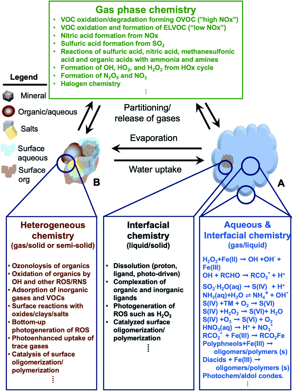
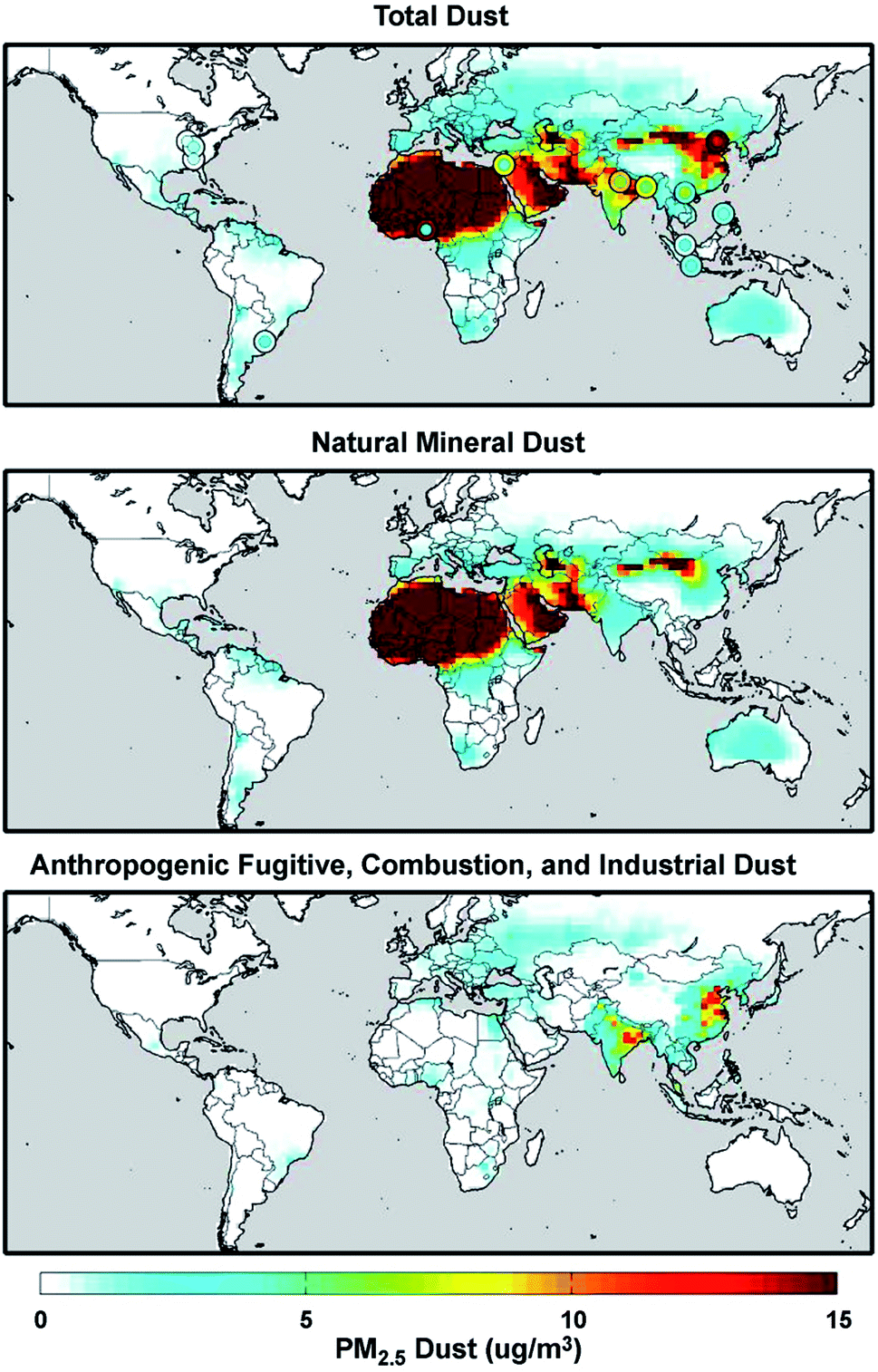
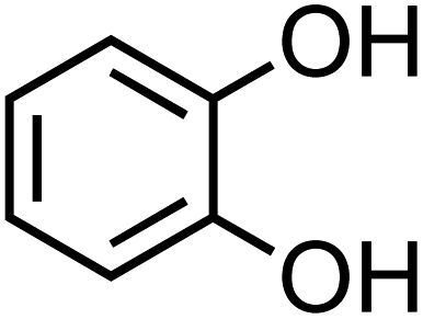
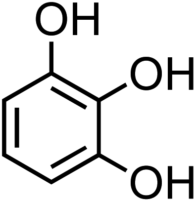
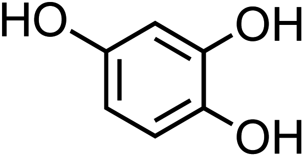
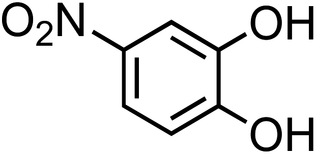
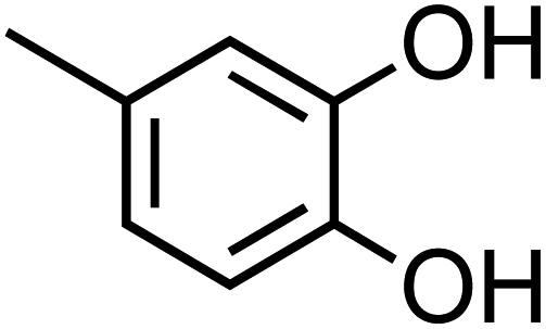
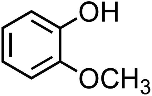
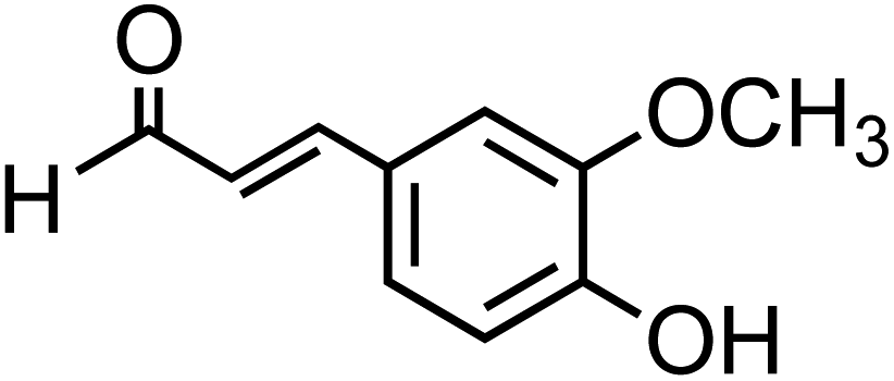
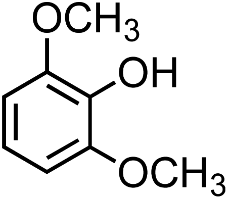
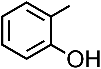
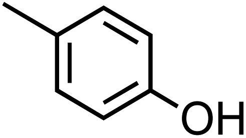
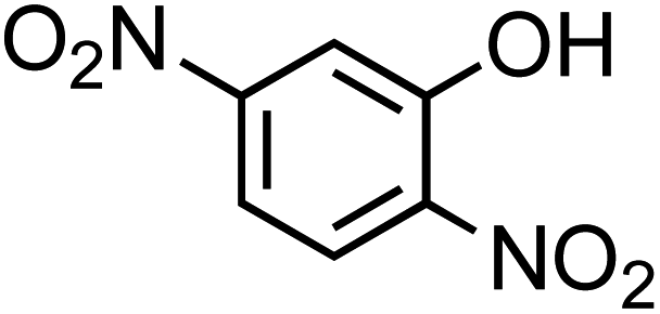

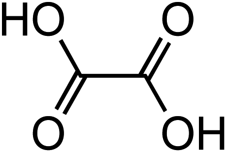
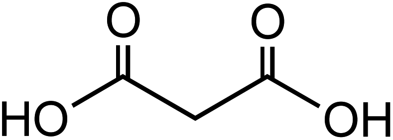
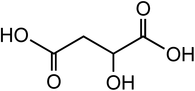
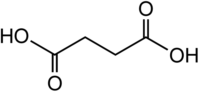
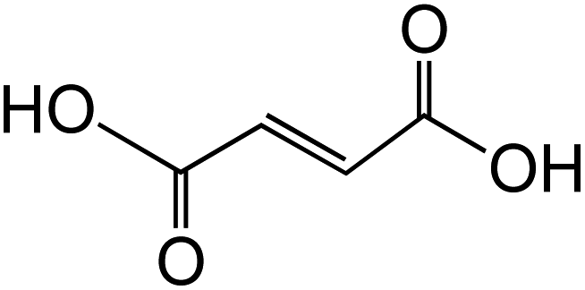
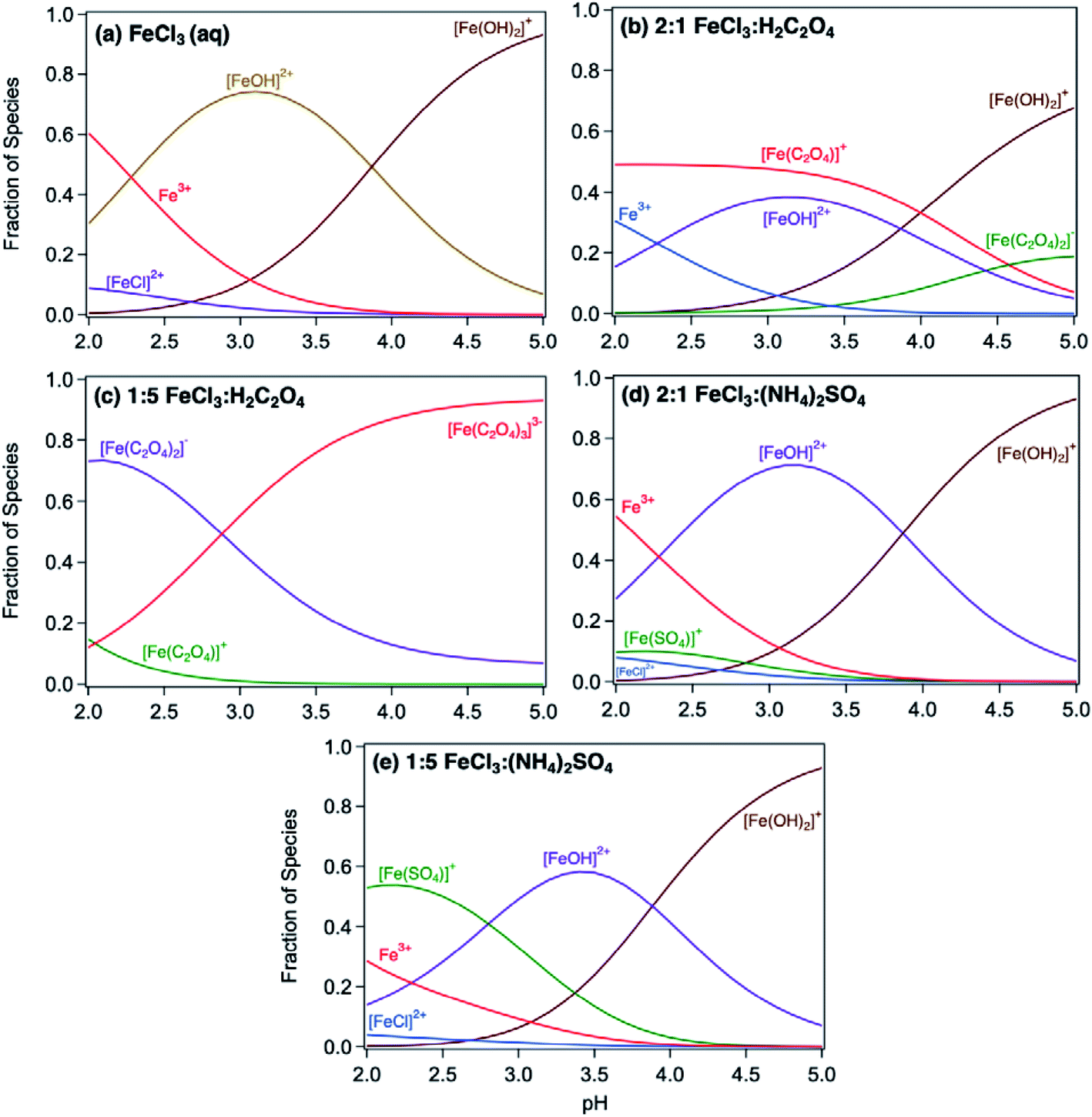


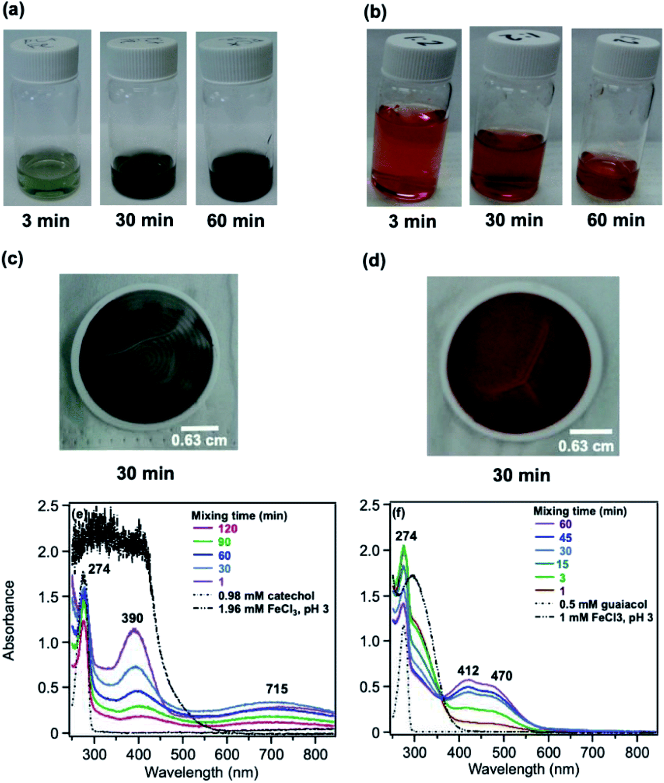

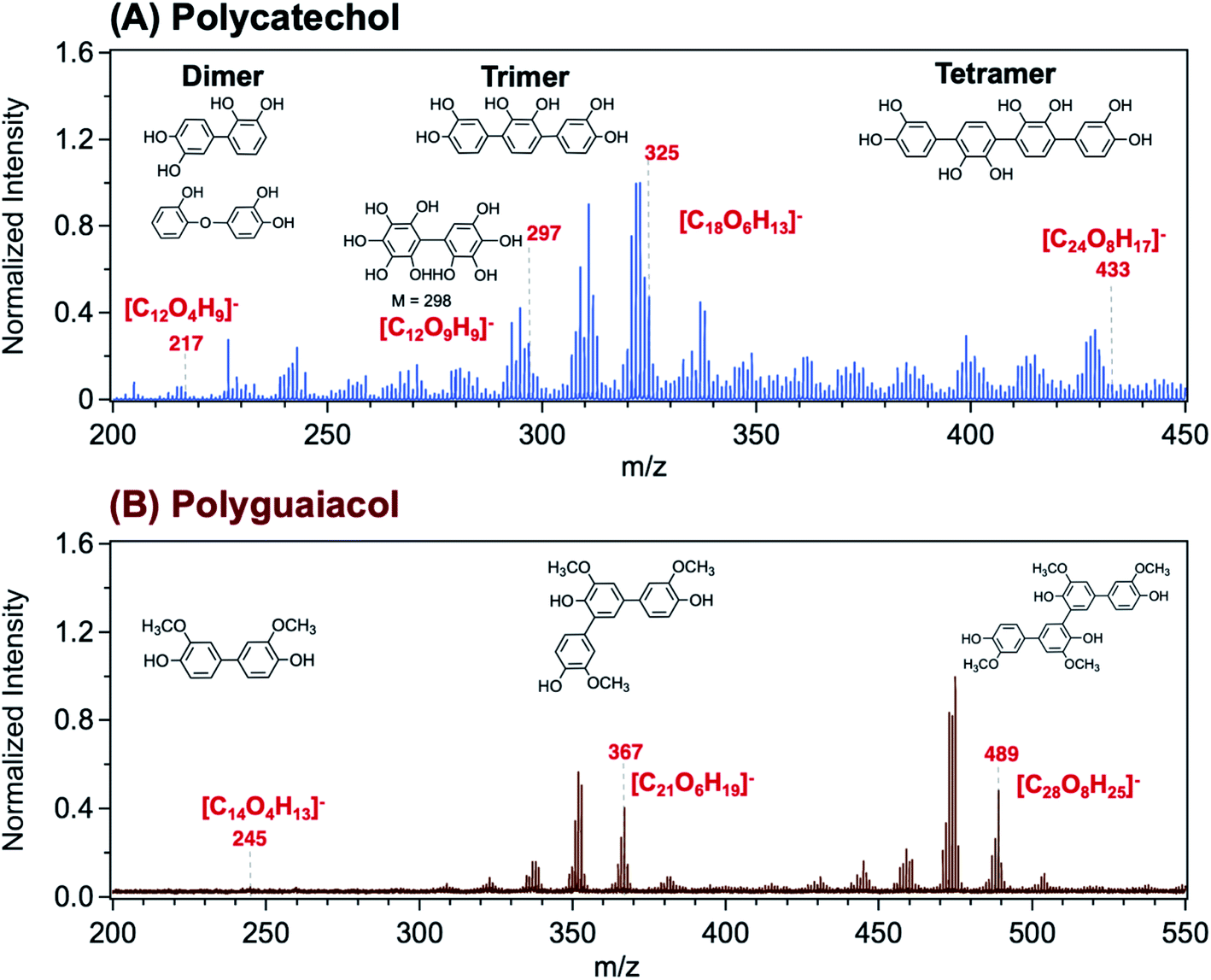
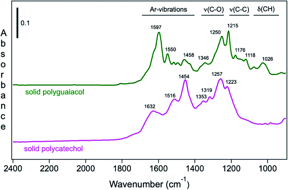
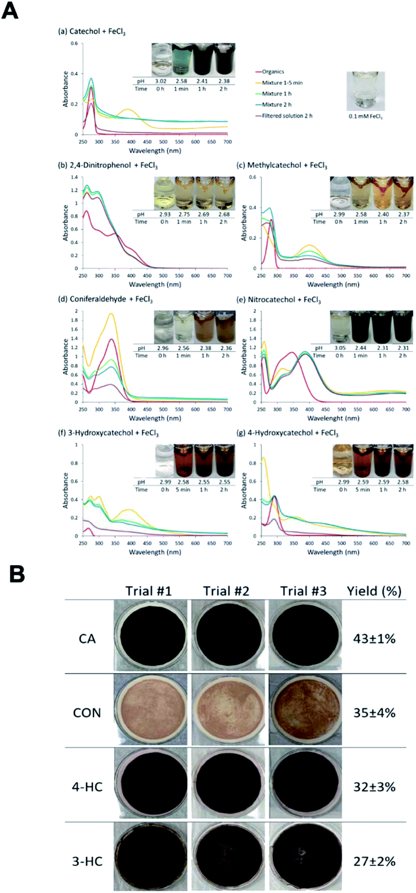
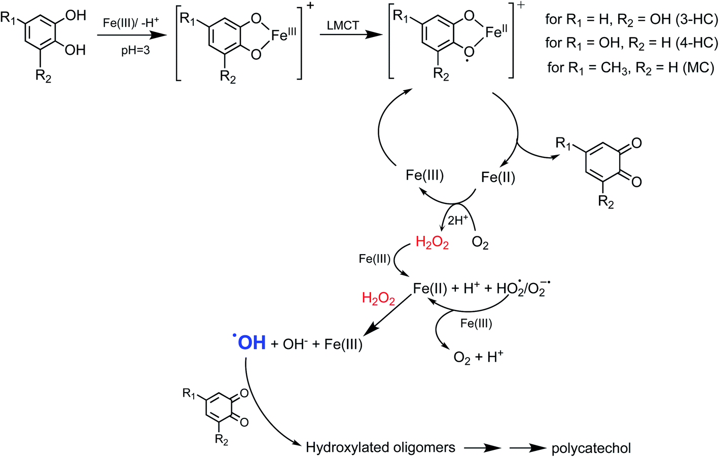
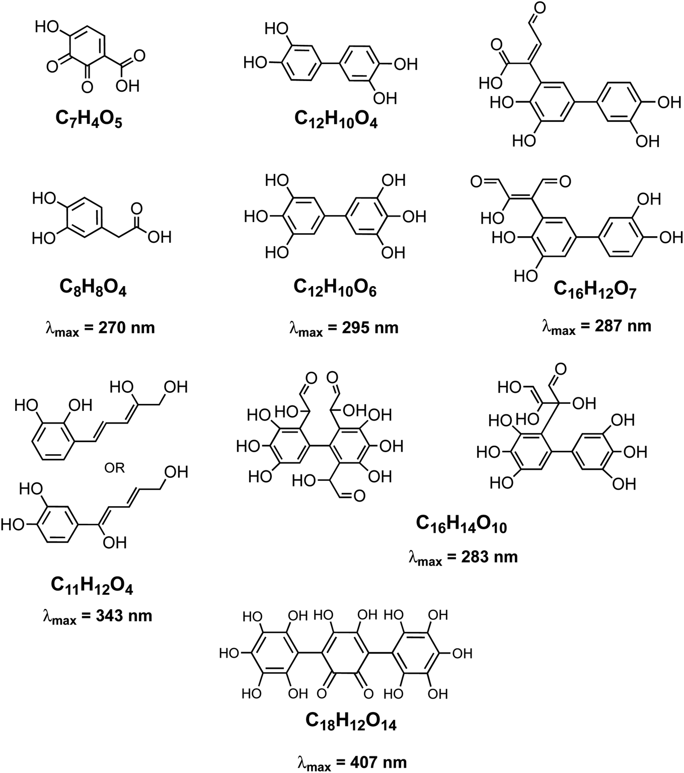

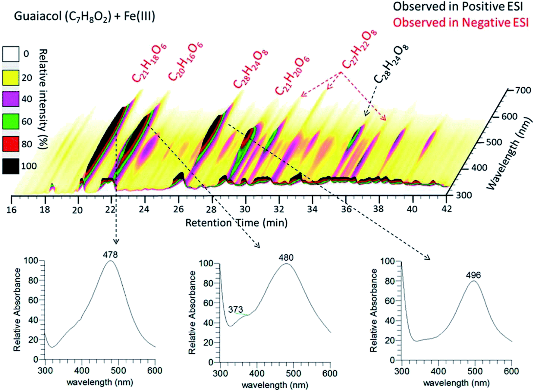
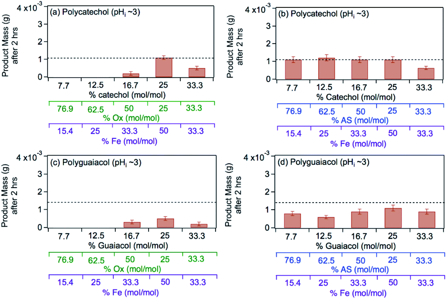
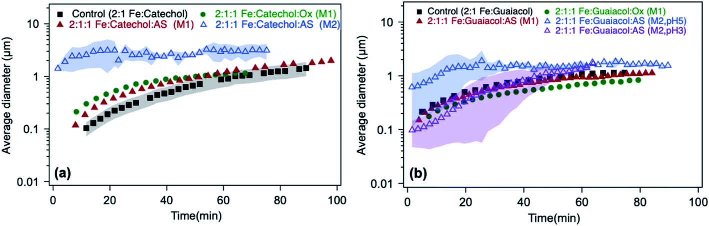
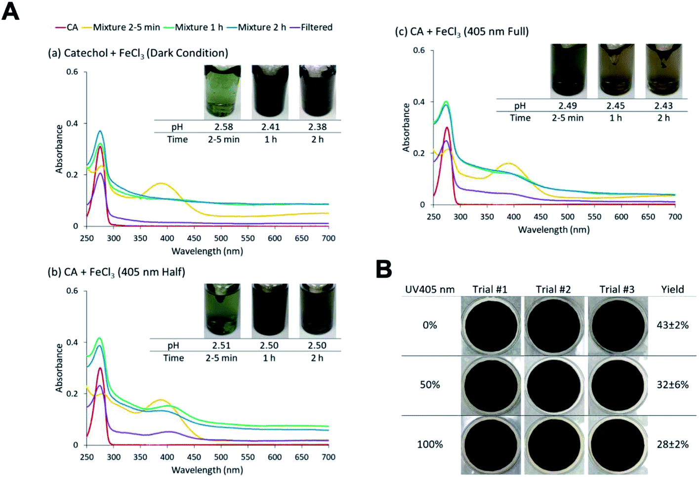
 , where Ci is the concentration of charged species in solution in molality (m) calculated using Visual MINTEQ182 for each solution.
b Calculated from the mass of a known volume.
c Measured in this study using a viscometer for low viscosity fluids. The ‘—’ indicates instrument was not accurate in measuring viscosity using water-like fluids around 1 mPa s.
d Calculated using E-AIM, Model IV, aqueous solutions.
e Calculated using Visual MINTEQ for each solution relative to total Fe(III) aqueous species in solution. Abbreviations are: Rxn = reaction, AS = ammonium sulfate, Org = organic compound, SA = succinic acid, MA = malic acid, GA = glutaric acid, and Mal = malonic acid. M1–3 refer to the number of organic compounds in the solution per the terminology used by Marcolli et al.180 The concentrations are in the final solutions after mixing. All solutions contained final concentrations of 2 × 10⁻³ and 1 × 10⁻³ M of Fe(III) and catechol, respectively. The final solution volume of Rxn no. 1–8 was 20 mL and of Rxn no. 9–11 was 5 mL. The ‘*’ marks the reactions that were analyzed using UHPLC-UV-MS after filtration.
, where Ci is the concentration of charged species in solution in molality (m) calculated using Visual MINTEQ182 for each solution.
b Calculated from the mass of a known volume.
c Measured in this study using a viscometer for low viscosity fluids. The ‘—’ indicates instrument was not accurate in measuring viscosity using water-like fluids around 1 mPa s.
d Calculated using E-AIM, Model IV, aqueous solutions.
e Calculated using Visual MINTEQ for each solution relative to total Fe(III) aqueous species in solution. Abbreviations are: Rxn = reaction, AS = ammonium sulfate, Org = organic compound, SA = succinic acid, MA = malic acid, GA = glutaric acid, and Mal = malonic acid. M1–3 refer to the number of organic compounds in the solution per the terminology used by Marcolli et al.180 The concentrations are in the final solutions after mixing. All solutions contained final concentrations of 2 × 10⁻³ and 1 × 10⁻³ M of Fe(III) and catechol, respectively. The final solution volume of Rxn no. 1–8 was 20 mL and of Rxn no. 9–11 was 5 mL. The ‘*’ marks the reactions that were analyzed using UHPLC-UV-MS after filtration.