Insights into the molecular composition of semi-volatile aerosols in the summertime central Arctic Ocean using FIGAERO-CIMS

Abstract

The remote central Arctic during summertime has a pristine atmosphere with very low aerosol particle concentrations. As the region becomes increasingly ice-free during summer, enhanced ocean-atmosphere fluxes of aerosol particles and precursor gases may therefore have impacts on the climate. However, large knowledge gaps remain regarding the sources and physicochemical properties of aerosols in this region. Here, we present insights into the molecular composition of semi-volatile aerosol components collected in September 2018 during the MOCCHA (Microbiology-Ocean-Cloud-Coupling in the High Arctic) campaign as part of the Arctic Ocean 2018 expedition with the Swedish Icebreaker Oden. Analysis was performed offline in the laboratory using an iodide High Resolution Time-of-Flight Chemical Ionization Mass Spectrometer with a Filter Inlet for Gases and AEROsols (FIGAERO-HRToF-CIMS). Our analysis revealed significant signal from organic and sulfur-containing compounds, indicative of marine aerosol sources, with a wide range of carbon numbers and O : C ratios. Several of the sulfur-containing compounds are oxidation products of dimethyl sulfide (DMS), a gas released by phytoplankton and ice algae. Comparison of the time series of particulate and gas-phase DMS oxidation products did not reveal a significant correlation, indicative of the different lifetimes of precursor and oxidation products in the different phases. This is the first time the FIGAERO-HRToF-CIMS was used to investigate the composition of aerosols in the central Arctic. The detailed information on the molecular composition of Arctic aerosols presented here can be used for the assessment of aerosol solubility and volatility, which is relevant for understanding aerosol–cloud interactions.

---

Environmental significance

The central Arctic during summertime has a very pristine atmosphere with very low aerosol particle concentrations. However, this is expected to change with climate change, as the extent of sea ice decreases. The number, size and chemical composition of aerosol particles are of importance for cloud formation, and hence for model projections of the Arctic climate. We have analysed the semi-volatile fraction of aerosol samples collected close to the North Pole in September 2018 at molecular level. This detailed information about aerosol properties is a crucial part for better understanding the Arctic aerosols and their influence on the climate in this vulnerable region.

1 Introduction

The polar regions are undergoing rapid transformation due to climate change. Global climate models¹ predict that the Arctic Ocean might be ice free in the summer by the end of the 21^st century as a result of anthropogenic greenhouse gas emissions.² As the contact area between the ocean surface and atmosphere expands due to the melting of sea ice, fluxes of particles and volatile compounds between the ocean and the atmosphere are likely to undergo changes. Such fluxes constitute an important local source of aerosol particles and particle precursors to the boundary layer (BL) in the central Arctic Ocean (roughly >80°N). Aerosol particles influence the climate, as they can scatter and absorb radiation^3–5 and interact with clouds.^5,6 Aerosol-cloud interactions play an important, yet poorly understood role in the changing Arctic climate.^7–10 Aerosols can, to a varying extent, act as cloud condensation nuclei or ice nucleating particles (CCN or INP). Their ability to do so depends on their size, morphology and chemical composition,¹¹ as well as ambient supersaturation. Aerosol particles can either be directly emitted to the atmosphere (called primary aerosols), or be formed or processed in the atmosphere via trace gases (secondary aerosols). As such, an improved knowledge of the sources, detailed chemical composition, and physicochemical properties of aerosols and their precursors is an important step for a better understanding of how the Arctic climate will respond to global warming.¹²

Aerosol mass loadings in the Arctic show a strong seasonal behaviour, with higher loadings in winter and early spring due to a phenomenon called Arctic haze,^13,14 where pollution from Eurasia and North America is transported to the Arctic.^15–17 During this time period, aerosol particles are mainly composed of sulfate (SO₄²⁻) and organic matter (Org), but also black carbon (BC), ammonium (NH₄⁺), nitrate (NO₃⁻), dust, and heavy metals.¹⁸ During the summer months (May–September), local sources become more important, as synoptic-scale transport from the south is less frequent, and air masses arriving in the Arctic have passed over open ocean in the North Atlantic and Pacific Oceans. As a consequence, these air masses have experienced more frequent precipitation, and therefore transport less aerosol mass to the Arctic compared to wintertime.^19–22

Our current understanding of aerosol sources and composition in the central Arctic is primarily the result of a series of icebreaker expeditions during the last three decades that were dedicated to atmospheric measurements. These took place in the summers of 1991 (IAOE-91),²³ 1996 (AOE-96),²⁴ 2001 (AOE-2001)^25,26 and 2008 (ASCOS).²⁷ Observations from these expeditions have e.g. shown sea spray aerosol (SSA) to be an important source for primary Arctic aerosol particles. SSA is a complex mixture of sea salt and organic matter,^28,29 and can also contain a fraction of semi-volatile organic compounds (SVOCs).³⁰ SSA are produced by bubble bursting following wave breaking in the ocean. These aerosols can be transported to the inner parts of the Arctic,³¹ or be emitted locally in leads between ice floes.³² Water-insoluble organic components (marine polymer gels) from the sea surface microlayer (SML) of open leads have previously been observed in Arctic clouds.^33,34 Aerosols produced by bubble bursting at both the ocean surface and from the surface of leads in the pack ice could therefore be a contributor to the central Arctic CCN budget.

Secondary organic aerosols (SOA) formed from organic volatile compounds have, through land-based studies in Alaska³⁵ and the Canadian archipelago^36,37 and ship-based measurements in the central Arctic Ocean,³⁸ shown to also make up a significant fraction of the submicron aerosol mass in the Arctic. These aerosols originate from both marine biogenic sources and long-range transport from continental areas. Among the trace gases important for SOA formation in the marine boundary layer (MBL) is dimethyl sulfide (DMS; C₂H₆S), a gas which is produced by phytoplankton and, in the polar regions, by sea ice algae.³⁹ DMS is oxidised in the atmosphere to products (e.g. sulfuric acid, SA; H₂SO₄ and methanesulfonic acid, MSA; CH₃SO₃H) with a low enough volatility and high enough hygroscopicity to be able to participate in the generation of CCN.^40,41 Recently, a new oxidation product of DMS, hydroperoxymethyl thioformate (HPMTF; C₂H₄O₃SO), was discovered.⁴² However, to what extent this gaseous compound can contribute to aerosol mass or growth has yet to be determined.

Although there is a general acceptance of a clear link between DMS oxidation and CCN formation over marine regions (see Charlson et al.⁴³ and e.g. reviews by Ayers and Carney⁴⁴ and Green and Hatton⁴⁵), the theory has been increasingly scrutinised and criticised for being too simplistic. Given the variety of particle types and potential aerosol precursor gases emitted in the MBL, DMS likely plays a more limited role in CCN formation than previously thought.^46,47 More recent studies have however provided new evidence for the relationship between DMS and Arctic SOA formation,^48–50e.g. relatively high MSA-to-sulfate ratios during aerosol growth and correlations between MSA and new particle formation (NPF) events. Knowledge about other SOA precursor gases and compounds has remained limited, since relevant measurements in this region are very scarce.⁵¹ This is particularly true for the central Arctic where access requires dedicated infrastructure such as icebreakers. Most research in the Arctic has therefore been conducted in the lower Arctic closer to the continental areas. In the Beaufort Sea in the Canadian Arctic, Fu et al.⁵² discovered that oxidation products of isoprene and α-pinene, commonly found in terrestrial SOA, were the dominant biogenic tracers of marine secondary aerosols. Other volatile compounds detected in the lower Arctic that could potentially contribute to SOA formation include formic acid and acetic acid.^53,54 However, to what extent these observations are applicable to the central Arctic is uncertain due to the increasing distance to land masses closer to the North Pole.

Detailed information on aerosol chemical composition can be used to derive SOA origin, as well as climate–relevant parameters such as hygroscopicity or volatility. In general, less volatile compounds have a higher elemental oxygen–carbon (O : C) ratio^55,56 and exhibit more complex and larger molecular structures.⁵⁵ Further, a low O : C ratio of bulk organic aerosol indicates a large fraction of aliphatic or lipid-like compounds with low solubility and hygroscopicity, whereas a high ratio corresponds to more oxidised and carbohydrate-like compounds with higher solubility and hygroscopicity, e.g. polysaccharides.²⁹ Molecular-level composition data can thus enable calculations of e.g. the hygroscopicity parameter κ,⁵⁷ which can provide a more accurate quantification of CCN ability, or improve volatility basis sets (VBS)^58,59 formulations, which are used to predict partitioning of compounds between the gas- and particle phase. Such numbers are largely not available for the central Arctic Ocean.

In this study, we analysed the aerosol chemical composition of 12 filter samples collected close to the North Pole between 11–19 September 2018 during the MOCCHA (Microbiology-Ocean-Cloud-Coupling in the High Arctic) campaign on the Swedish Icebreaker (I/B) Oden using a High Resolution Time-of-Flight Chemical Ionization Mass Spectrometer with a Filter Inlet for Gases and AEROsols (FIGAERO-HRToF-CIMS, Aerodyne Research Inc., USA⁶⁰) and iodide (I⁻) as the reagent ion, hereafter referred to as FIGAERO-CIMS. The samples were collected when Oden was moored to an ice floe in the central Arctic Ocean, as well as on its transit back to the marginal ice zone (MIZ). The results provide insights into the molecular composition of secondary aerosol components and the volatile organic fraction of primary aerosols. To our knowledge, this is the first time this technique was used for aerosols from the central Arctic.

2 Methods

2.1 The MOCCHA campaign

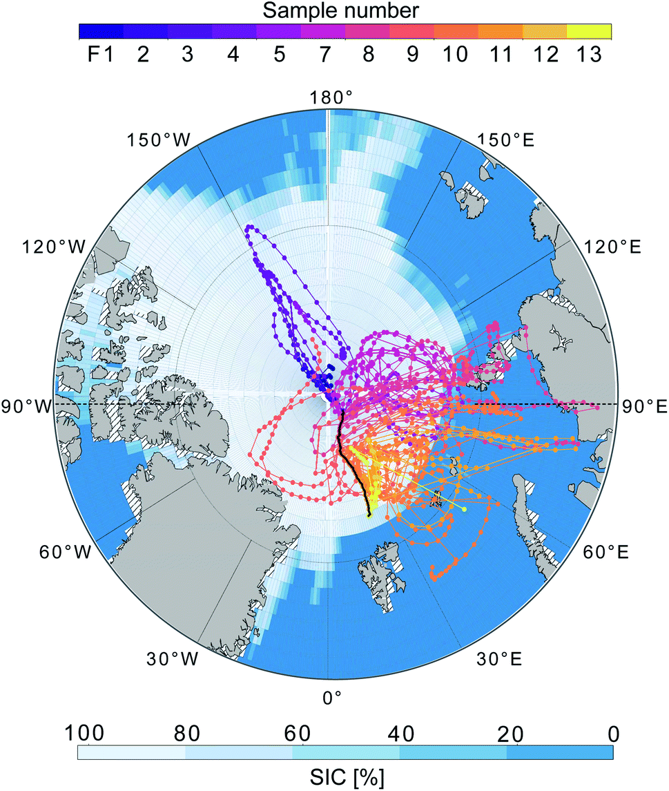
The MOCCHA campaign was part of the research expedition Arctic Ocean 2018 with the Swedish Icebreaker (I/B) Oden in August and September 2018. During a period of almost 5 weeks (13 August–14 September 2018), between the central Arctic summer and the autumn freeze-up, the icebreaker was moored to an ice floe close to the North Pole (89°N) and drifted with the pack ice. During these weeks, measurements from the ship and the ice floe were conducted. The general research question MOCCHA aimed to answer was to what extent marine microbiology contributes to local aerosol emissions and cloud formation.⁶¹

The cruise with I/B Oden started from Longyearbyen, Svalbard (78.2°N, 15.6°E) on 1 August 2018 and returned to the same location on 22 September 2018 as shown in Fig. 1. During the ice camp, I/B Oden drifted from 89.6°N, 40.6°E to 88.5°N, 36.7°E. During both the transit north- (August) and southward (September), the ship was moored for sampling in the MIZ during 24 h (referred to as MIZ stations). The aerosol samples analysed for this study were collected in September during the autumn freeze-up (red track in Fig. 1). Logistical issues prevented samples from being collected during the entire expedition period. Details on filter sampling periods and corresponding locations are presented in Table 1. All dates and times are given in UTC.

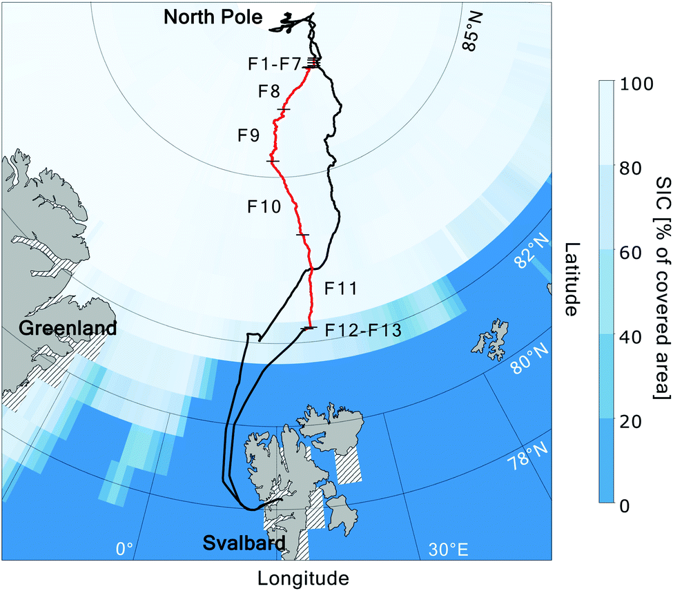Fig. 1 Route of I/B Oden during the Arctic Ocean 2018 expedition, with the position during the filter sampling period highlighted in red. Black numbers correspond to sample (filter) numbers, from the ice floe close to the North Pole (F1–F7), during the transit southward through the pack ice (F8–F11), to the marginal ice zone (F12–F13). Black short lines indicate sampling start and end positions. Sea ice concentration (SIC; Met Office Hadley Centre⁶²) for September 2018 is shown as percentage of covered area. Hatched areas around the land areas represent missing SIC data.

Table 1 Summary of sampling times, with start and end time given as month and day (e.g. 09–11) in year 2018, and time of day in UTC (e.g. 14:00), locations and sampling conditions of the aerosol filter samples. F1–F13 are ambient samples, B1 and B2 are field/handling blanks. All coordinates are given as degrees North, degrees East (°N, °E). The ship contamination column gives an estimation of the probability that the sample was contaminated by ship emissions, where 0 – very low risk (no contaminated air entered the inlet), 1 – low risk (contamination was effectively removed by the pollution control system), 2 – moderate risk (not all contamination was removed by the pollution control system), 3 – high risk (contaminated sample). The procedure for determining the risk of contamination is described in Section 2.5

Sample	Start time	End time	Start coord.	End coord.	Sample duration (h)	Sampling conditions	Ship contamination
F1	09–11 14:00	09–11 23:24	88.6, 45.0	88.6, 44.1	9.4	Ice floe	0
F2	09–11 23:26	09–12 07:49	88.6, 44.1	88.5, 43.2	8.4	Ice floe	0
F3	09–12 07:51	09–12 14:34	88.5, 43.2	88.5, 42.3	6.7	Ice floe	0
F4	09–12 14:44	09–12 22:22	88.5, 42.3	88.5, 41.0	7.6	Ice floe	0
F5	09–12 22:26	09–13 07:50	88.5, 41.0	88.5, 39.6	9.4	Ice floe	0
F6	09–13 07:57	09–13 14:09	88.5, 39.6	88.5, 38.8	6.2	Ice floe	0
F7	09–13 14:12	09–14 13:34	88.5, 38.8	88.5, 38.1	23.4	Ice floe	1
B1	09–14 13:44	09–14 13:44	88.5, 38.8	88.5, 38.1	N/A	Ice floe	N/A
F8	09–14 13:44	09–15 15:34	88.5, 38.1	87.6, 18.6	25.8	Transit	3
F9	09–15 15:39	09–16 11:53	87.6, 18.5	86.4, 13.7	20.2	Transit	2
F10	09–16 11:48	09–17 23:06	86.4, 13.7	84.6, 21.4	35.3	Transit	2
F11	09–17 23:09	09–18 23:58	84.6, 21.4	82.4, 21.1	24.8	Transit	3
F12	09–19 00:10	09–19 14:27	82.4, 21.1	82.3, 20.4	14.3	MIZ	0
F13	09–19 14:33	09–19 23:35	82.3, 20.4	82.3, 20.1	9.0	MIZ	0
B2	09–19 23:44	09–19 23:44	82.3, 20.1	82.3, 20.1	N/A	MIZ	N/A

---

2.2 Particle sampling and offline analysis

2.2.1 Filter sampling. During 11–19 September 2018, 13 ambient aerosol samples (referred to as F1–F13) were collected during mooring to the ice floe (the ice drift), when the ship was steaming southward (transit), and in the MIZ station with the engines off (see Table 1). In addition, 2 field blanks (B1–B2) were taken during transit and in the MIZ. Aerosols were sampled via deposition onto pre-baked (24 h at 200 °C) 24 mm Zefluor®PTFE filters (Pall Corporation, USA) placed in a 25 mm stainless steel filter holder (Sartorius Lab Instruments, no. 16251, Germany). Sample air was drawn at 90 litres per minute (lpm) through a whole-air inlet (3 in. o.d., length 4 m) located at 25 m above sea level (4^th deck of I/B Oden) to capture aerosols, cloud and fog droplets. The filter holder was connected to the main inlet line via a 60 cm long stainless steel tube (1/4 in. o.d.) and two short pieces of conductive silicone tubing (3/8 and 1/4 in. o.d., total length 25 cm), the sample flow was 1.05 lpm (F1–F3) and 3.18 lpm (F4–F13). Controlled heating (30–40 °C) of the inlet prevented clogging of the inlet with ice. In addition, inlet heating led to evaporation of cloud and fog droplets, so that all aerosol particles, whether activated or not, were included in the measurement. Total residence time in the inlet was <1.5 s. Inlet particle number losses were calculated to be ∼1–8% for smaller particles with diameters D_p = 0.01–1 μm (∼0.5–1% for the accumulation mode, D_p = 0.1–1 μm), and ∼1–75% for larger particles with D_p = 1–10 μm using the Particle Loss Calculator described in Von der Weiden et al.⁶³ with a particle density of 1.30 g cm⁻³ (see explanation on how this value was derived in Section 2.3). We assume however that the majority of the compounds measured by FIGAERO-CIMS are in the submicron range. Filter collection times were in the range of 6.7–35.3 h (Table 1), depending on atmospheric conditions such as changes in air mass origin or particle number concentrations. Field blanks were prepared in the exact same way as the samples and placed in the sample holder with the pumps turned off to not allow any ambient air to be drawn through the filter. The blanks did not sit in the holder for a longer time, but were simply loaded and unloaded as the majority of the contamination is assumed to come from handling of the filter and equipment. After the deposition, the filters were wrapped in aluminum (Al) foil and stored frozen until analysis.

2.2.2 FIGAERO-CIMS analysis. The filter samples were analysed with a FIGAERO-CIMS in the laboratory at Stockholm University, Sweden. Using the FIGAERO-CIMS with filters collected outside of the instrument (“offline mode”) corresponds to only using the particle-phase (p) analysis function of the FIGAERO, as described by Huang et al.⁶⁴ Sample F6 was omitted to allow for later analysis by other analytical methods (not part of this study). Sample F6 was chosen since it was collected under similar conditions (in terms of the ice drift and sampling duration) to samples F1–F5. The samples collected during the transit (F8–F11) had elevated risk of contamination from ship emissions (Table 1), which were identified based on particle number concentration/distribution and BC measurements (see description in Section 2.5).

Particle analysis in the FIGAERO-CIMS proceeds as follows: particles collected on the filter are evaporated by a flow of nitrogen (N₂) that is gradually heated from room temperature to 200 °C during 20 min and then kept at 200 °C for another 20 min to allow the sample to fully evaporate off the filter. Therefore, compounds that do not evaporate at 200 °C (e.g. sea salt, volume fraction remaining of sea salt heated to 200 °C > 0.9 ⁶⁵) or decompose at <200 °C cannot be directly detected by this method. Inside the ion–molecule reaction region (IMR), the volatilised compounds are ionised by iodide ions (I⁻) via adduct formation.^66–68 The negatively charged ions are then separated according to their time of flight (ToF) in the mass spectrometer, from which their mass-to-charge (m/z) ratio can be inferred using known ions as calibrants. This procedure allows for the characterisation of evaporated particulate compounds at molecular level (accuracy ≤4 ppm).

In total, we were able to identify 1586 ions, whereof 519 were clustered with I⁻. For the analysis in this study, only compounds clustered with I⁻ were used, as the ionisation mechanism of ions not clustered with I⁻ is less clear. Ion signals were normalised to the reagent ion signal (I⁻, m/z 126.905). The normalised time series of an individual ion was then integrated over the heating time, and the integrated signal (number of ions) was converted to moles, normalised to the sampling volume and weighted by the compound's molar mass (M, g mol⁻¹). As such, the unit of the data presented here is M-weighted signal per sampled volume in g m⁻³, not atmospheric concentration.

Total subtracted backgrounds consisted of instrument background and field blank. Instrument backgrounds were determined by repeating the heating cycle of each filter (i.e. each filter was heated twice), and the signal of the second heating (instrument background) was subtracted from the signal of the first heating. The same approach was used for the two field blanks B1 and B2. As field blank for the entire study, the mean of the difference in signal between the first and the second heating of the two field blanks was used (a comparison of these is shown in Fig. S1†). For B1, F8 and F12, the time series of the second heating had a higher baseline compared to the first heating, which led to negative values when subtracting the second heating. For B1, this was corrected for by aligning the baselines of the two heatings (Fig. S2†). For F8 and F12, the instrument backgrounds were approximated by the average background signal (second heating) of B1 and B2 (Fig S3†). For these two filter samples, the instrument background therefore represents a lower limit. Limit of detection (LOD) for the background-subtracted signals was determined as 1 standard deviation (1σ = 7.060 × 10⁻¹⁹ g m⁻³) of the field blanks average signal of all ions,⁶⁹ with outliers removed. The outliers are shown in Table S1† and the percentage of signal remaining after exclusion of compounds <LOD in Table S2.†

2.3 Online particle measurements

Measurements of non-refractory submicron organic (Org) and sulfate (SO₄²⁻) particulate matter were performed using a High Resolution Time-of-Flight Aerosol Mass Spectrometer (HR-ToF-AMS, Aerodyne Research Inc., USA^70,71) connected to either the whole-air or an interstitial inlet with a particle cutoff size of 1 μm in aerodynamic diameter (PM₁) through the use of a switching mechanism. More details about the instrument can be found in Canagaratna et al.⁷¹ and Schmale et al.⁷²

Particle volume in the size range 10–921 nm was determined from aerosol number size distributions measured by a differential mobility particle sizer (DMPS), consisting of a custom built medium Vienna type differential mobility analyser (DMA; effective length 0.28 m, inner radius 0.025 m, outer radius 0.0335 m) together with a mixing condensation particle counter (MCPC; Brechtel Manufacturing Inc., Model 1720, USA), and a WELAS®2300HP white-light aerosol spectrometer with a Promo®2000H system (Palas GmbH, Germany). WELAS data were used for particles with a diameter >300 nm. Above this diameter, the DMPS signal is influenced by multiply charged particles, which can significantly contribute to the total particle volume. For both instruments, the data were corrected for diffusion, impaction and sedimentation losses using the Particle Loss Calculator as described by Von der Weiden et al.⁶³ assuming a common particle density (ρ) of 1.30 g cm⁻³ for submicron particles. This value represents the mean submicron particle density based on the relative contributions to AMS mass from Org (ρ ≈ 1.22 g cm⁻³ based on the density of β-caryophyllene SOA as representative of more complex/primary SOA⁷³), and non-sea-salt sulfate (nss-SO₄²⁻; ρ ≈ 1.788 g cm⁻³, which is the density of H₂SO₄·H₂O).⁷⁴ Sea salt was not included in the density estimation based on findings by Chang et al.³⁸ showing that submicron sea salt concentrations were negligible in the central Arctic Ocean. The measured concentrations of ammonium (NH₄⁺), nitrate (NO₃⁻) and chloride (Cl⁻) were extremely low compared to Org and SO₄²⁻, and were hence not included in the particle density calculation. The estimated particle density was further used for converting the integrated submicron particle volume measured by the DMPS and WELAS to mass concentrations.

Another MCPC 1720 was used to measure total particle number concentrations. Concentrations of black carbon (BC) were derived from a multi-angle absorption photometer (MAAP, Thermo Scientific Inc., Model 5012, Germany⁷⁵). The MAAP measures light absorption at λ = 637 nm, which is the wavelength at which BC is the primary absorber.⁷⁶ DMPS, WELAS and MAAP were all connected to the whole-air inlet on the 4^th deck of the Oden.

2.4 Gas-phase measurements

DMS in ambient air was measured using an instrument developed at the Department of Meteorology, Stockholm University. Leck et al.²⁴ determined the overall accuracy to ±12% and provided a detailed description of the setup. The instrument was installed in a container on the ship's 4^th deck, at 25 m above sea level. Sample air was pumped into the lab inside the container and to the instrument via the PM₁ inlet. The flow through the white, low-transparent PTFE tubing (1/8 in. o.d., length ∼4 m from inlet to instrument) was 1.1 lpm. Inside the instrument, ozone (O₃) was removed from the sample air using a cotton scrubber, as described by Persson and Leck.⁷⁷ The cotton was replaced every 6 h to ensure efficient removal of O₃. Subsequently, the sample flow was passed through a tube containing gold (Au) wool onto which gas-phase (g) DMS was adsorbed for time periods of 15, 30 or 60 min depending on ambient concentrations. Two Au wool tubes were used and the sample flow was switched between them. The sampling time was adjusted to optimise for a large enough signal for integration and a high time resolution. Once adsorbed, accumulated DMS (g) was heated off of the Au wool and analysed by a gas chromatograph with a flame photometric detector (Hewlett-Packard, 19256A FPD, USA). Measurements were made continuously, with one break on 14 September (00:25–10:55) for calibration of the system. Another calibration was made after the sampling period on 20 September. For the samples, the calibration run that was closest in time was used. Calibration was made for nanograms of sulfur (DMS-S) through analysis of dry synthetic air with DMS released at a constant rate (47 ng DMS min⁻¹ at 30 °C) from a permeation device (Kin-Tek Analytical, Inc., USA). Since the calibration data of one of the Au tubes showed a very large spread, measurements made with it were excluded from the data set. Given this, the time series has a lower time resolution than if both gold tubes had been included. Data points at the beginning of each run and around the time for cotton exchange were removed as the system requires time to stabilise.

Ambient SA and MSA (g) were measured using a nitrate HR-ToF-CIMS (Aerodyne Research Inc., USA^78,79) through an inlet on the 4^th deck of I/B Oden. This inlet was designed to sample compounds relevant for NPF, i.e. with a short residence time to minimise diffusional losses during sampling. Due to its location closer to the ship deck and therefore increased potential for contamination from the ship's exhaust, more data points had to be removed compared to the other online instruments (for more information, see Baccarini et al.^80,81).

2.5 Pollution control

All inlets used during the expedition were pointed towards the bow of I/B Oden, which was turned upwind to minimise the risk of sampling pollution from the ship. The setup was similar as during the earlier cruises with I/B Oden (see Leck et al.²³ for details). All measurements except for the ambient DMS and the online aerosol instrumentation were further monitored by a pollution-detection system, which automatically switched off the pumps when the total particle count exceeded 3000 cm⁻³. The pumps were automatically restarted once the particle count was below the threshold value for at least 60 s. Additional checks for periods of contamination impacting the data were made after the campaign through manual comparison of particle number and BC concentrations (Fig. S4†) with the protocol for when the pumps had been turned on and off either manually or automatically by the pollution-detection system. The risk of contamination was also assumed to be higher when the ship was moving with its engines running (see “Transit” in Table 1). The filter samples are labeled with 0–3, where 0 – very low risk (no contaminated air entered the inlet), 1 – low risk (contamination was effectively removed by the pollution control system), 2 – moderate risk (not all contamination was removed by the pollution control system), 3 – high risk (contaminated sample). The labels are shown in Table 1.

2.6 Back trajectory analysis and meteorology

Five-day backward trajectories arriving at I/B Oden were calculated using the Lagrangian analysis tool LAGRANTO⁸² using wind fields from 3-hourly operational ECMWF (European Centre for Medium-Range Weather Forecasts) analyses, interpolated to a regular grid with 0.5° horizontal resolution and 137 vertical model levels. Trajectories initialised (t = 0) within the BL (where the number of levels ranged between 5 and 15 for individual trajectories) were averaged to a single trajectory. The mean height at the lowest level (1) was 8.3 m and maximum height (level 15, one trajectory) was 730 m. The mean height difference was 7.6 m between the lowest 5 levels, 39.0 m between each of levels 5–8 and 80.1 m between each of levels 8–15. An example showing the difference between the levels and the averaged trajectory can be found in Fig. S5.†

Information about meteorological conditions at the sampling position was obtained from the fixed instrumentation on-board the ship. Shortwave radiation data was gathered by the weather station installed on the 7^th deck of I/B Oden by the Department of Meteorology, Stockholm University.^83,84 Meteorological parameters along the trajectory were also provided by LAGRANTO.⁸² Monthly ice concentration data were obtained from the Met Office Hadley Centre.⁶² In this study we present some common parameters including air temperature and relative humidity, fog and cloud occurrence (Fig. S6†) and wind speed (Section 3.2). The air temperature was below 0 °C throughout the aerosol sampling period and the relative humidity (RH) was in general high (81.3–100%). Fog and cloud events occurred frequently, as is common in the Arctic at this time of the year.^85,86 Detailed descriptions of the meteorological conditions during the expedition are provided in Vüllers et al.⁸⁷ and Prytherch and Yelland.⁸⁸

3 Results and discussion

3.1 Particulate compounds measured by FIGAERO-CIMS

Our analysis revealed significant signal from organic compounds and contributions from sulfur-containing compounds in all filter samples from ice floe to transit and MIZ, in line with previous results showing organic compounds to make up a large fraction of submicron aerosol particles in the central Arctic Ocean during fall when local marine emissions prevail.³⁸ We grouped the 519 molecules clustered with I⁻, for which we determined their molecular composition, into different categories: the CHO group containing compounds with carbon, hydrogen, and oxygen atoms only; the CHON group with compounds also containing nitrogen; the CHOS group with compounds also containing sulfur; the CHONS group with compounds with both nitrogen and sulfur; halogen-containing compounds (Halogen); and inorganic sulfur-containing compounds (Inorg. S). Fig. 2a displays the background-subtracted median mass spectrum of all filter samples, where each stick represents the median signal of an individual ion (clustered with I⁻) above LOD. The different panels in Fig. 2a show the corresponding category a certain ion in the mass spectrum belongs to. Organic compounds (mainly CHO and CHON) were found over the entire spectrum, thus exhibit a large range of molecular sizes. CHOS compounds in general are molecules with a relatively short carbon backbone (number of carbons <9), but the addition of sulfur can still shift their m/z to the higher range of the spectrum. A detailed discussion on the molecular composition of individual compounds of the different categories follows in Section 3.2. The compounds in category Other were found mainly at m/z <127, showing that they were to large extent not clustered with I⁻ and consisted of smaller fragmentation products.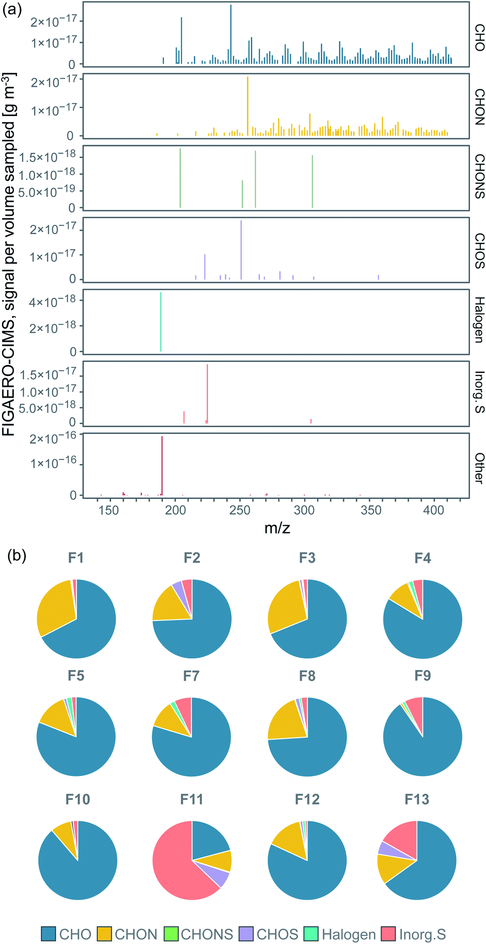

Fig. 2 (a) FIGAERO-CIMS high resolution mass spectrum of the sample median signal separated by compound category, showing where in the spectrum molecules of the different categories were found, (b) pie charts of the relative contribution to the total signal intensity (sampled mass per sampled volume) of the compound categories in each individual filter (the category Other not included). Percentages of the pie charts are listed in Table S3.†

The relative contribution to total mass (excluding Other) of each compound group for each individual filter is shown in the pie charts in Fig. 2b. The percentages of the pie charts can be found in Table S3.†CHO was commonly the dominating category, followed by CHON, CHOS, Inorg. S and CHONS. The main contributing compounds to the CHOS category were C₂H₄O₄S (m/z 250.888) and CH₃SO₃H (MSA; m/z 222.893). From Fig. 2a, they also stand out as two of the largest peaks of all compound categories, which is the reason why CHOS sometimes make up a relatively large fraction of the total mass (Fig. 2b). C₂H₄O₄S is not, in contrast to MSA, known as a common DMS oxidation product. It could however be possible that it is a reaction product between a DMS oxidation product and another atmospheric compound.

The Inorg. S category covers sulfuric compounds that are inorganic, largely consisting of H₂SO₄ (sulfuric acid; SA), H₂O(SO₃)₂ (disulfuric acid) and SO₃ (sulfur trioxide). These compounds can originate from DMS oxidation, long-range transport of sulfur compounds emitted by non-marine sources or ship exhaust. The latter source may have contributed when the ship was steaming southward on 14–19 September (F8–F11, Table 1). We will further discuss this in Section 3.3. The Halogen category includes compounds that contain halogen atoms, where only C₂FH₃O was above LOD. The Other category contained e.g. nitric acid (HNO₃, m/z 189.900, 78.9% of the sampled mass), followed by other inorganic compounds made up of oxygen, hydrogen and/or nitrogen.

3.2 Temporal evolution of particle measurements

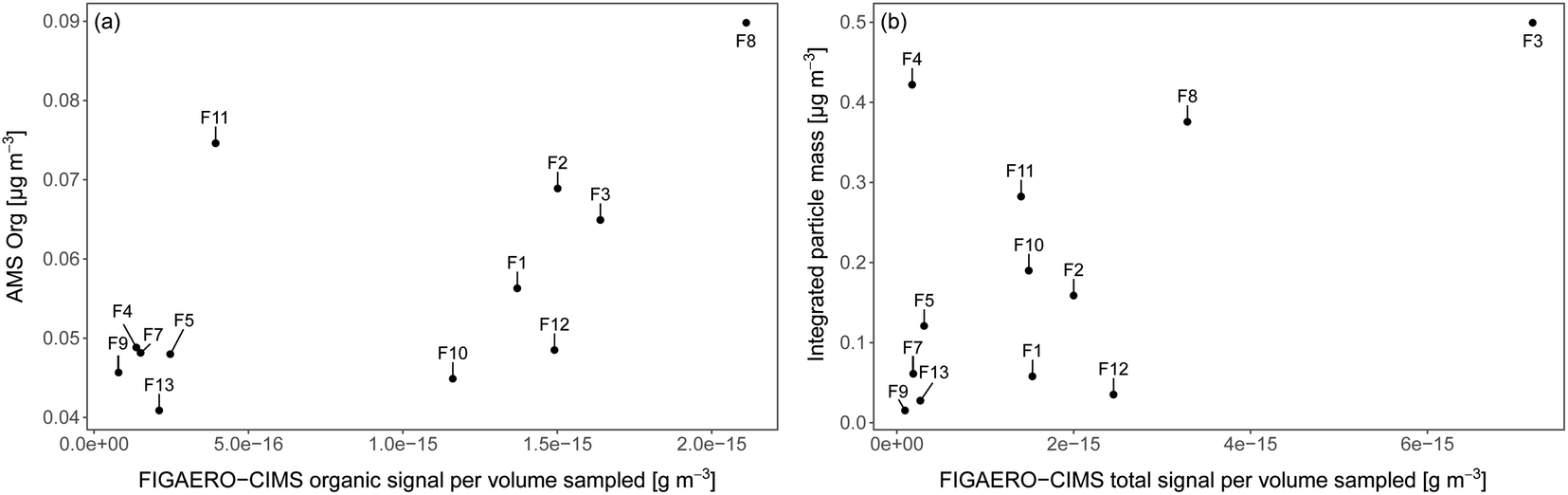
As the iodide FIGAERO-CIMS measures a subset of atmospheric organic components and is more sensitive to e.g. oxygenated molecules, it is useful to compare the signal from the FIGAERO-CIMS to concurrent measurements of particle chemical composition. Fig. 3a and b show the time series of the total signal intensity for each FIGAERO-CIMS category in each sample across the entire sampling period along with the mass concentrations of sulfate (SO₄²⁻) and organics (Org) measured by the AMS, as well as submicron particle mass concentrations derived from DMPS and WELAS size distributions (aggregated to the filter sampling periods). Scatterplots of Org and particle mass concentrations with total signal measured by FIGAERO-CIMS are shown in Fig. 4. Inorganic ammonium, nitrate and chloride from AMS were not included in the analysis as their concentrations were extremely low compared to Org and SO₄²⁻ and close to the detection limit.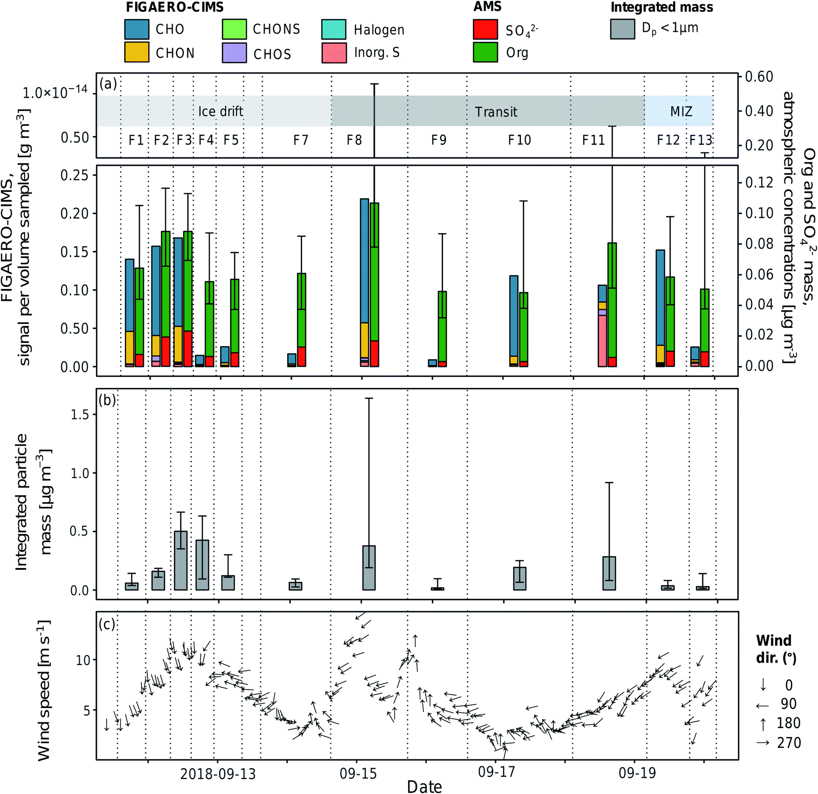

Fig. 3 Time series of (a) the summed aerosol sample signal separated by compound categories (analysed by FIGAERO-CIMS), median mass concentrations of organic (Org) and sulfate (SO₄²⁻) aerosols (analysed by AMS) per filter sampling periods, (b) integrated particle mass of submicron aerosols per filter sampling periods, and (c) wind speed and direction (30 min average). The error bars represent the 25^th and 75^th percentiles. Sample names (F1–F13) are shown above the bars and their start and end times are represented by the dashed vertical lines. The shaded areas in the top panel show the sampling conditions (see also Table 1).

Fig. 4 Relationship between (a) total signal from organic compounds of each FIGAERO-CIMS sample and organic mass sampled by AMS aggregated to the filter sampling periods, (b) total signal of each FIGAERO-CIMS aerosol sample and the integrated particle mass of submicron aerosol aggregated to the filter sampling periods. F1–F13 are the sample numbers.

All techniques qualitatively observe the same pattern: relatively higher concentrations on the ice floe and in the end of the sampling period close to the MIZ, as well as another peak mid-period during transit, and lower concentrations in between. Particle mass concentrations were in general smaller as the air mass became more marine in nature during the second half of the measurement period. This was especially clear for F12–F13, collected in the MIZ and with the air mass coming from over the Barents Sea, and hence being highly marine in nature (Fig. 5). As there were no apparent differences in precipitation, temperature and relative humidity along the trajectories (data not shown), the contrast in sampled mass was probably a result of different particle sources. The higher values (mainly F3, F4, F8 and F11) are relatively well aligned with the peaks in wind speed (Fig. 3c). This could mean that higher wind speeds increase local emissions of large primary aerosols by sea spray in the pack ice leads, although this needs further investigation and a larger data set to state for sure. However, there was a shift in particle size distribution and contribution of larger particles during the F3 and F4 periods (Fig. S7†), which led to an increase in total particle mass not observed by AMS and FIGAERO-CIMS. This could be an additional indication of increased local sea spray particle emissions, as the AMS and CIMS are less sensitive to primary SSA particles. There was also a distinct drop in FIGAERO-CIMS signal as the wind direction changed from mainly northerly (0°) during 11 and 12 September to mainly easterly (90°) from 13 to 19 September. This coincided with a change in air mass origin (Fig. 5). On a local level (immediately at the sampling site), no clear correlation to other meteorological parameters could be identified (see Fig. S6†).

Fig. 5 5-day backward trajectories arriving at I/B Oden during 11 September 00:00 UTC-20 September 00:00 UTC (one trajectory starting every 3 hours). The map shows the position of I/B Oden (black line) and the trajectories are coloured by sample number. Sea ice concentration (SIC) for September 2018 is shown in blue scale.

The air sampled in F1–F3 originated mainly from the pack ice region toward the Beaufort Sea. Out of the filter samples from the ice drift, F1–F3 had higher signals compared to F4–F7, with air masses coming from the pack ice/open waters toward the Siberian coast. The relative contribution of CHO and CHON was also more similar in F1–F3 compared to F4–F7 (see Table S3†), although this is most likely affected by the reduced number of compounds above LOD at lower overall signal intensity. Similar composition between samples could indicate similar source profiles and/or that they are part of the same air mass(es) subject to the same meteorological conditions.

The highest relative and absolute signal from Inorg. S by the FIGAERO-CIMS was found in F11, which was influenced by ship contamination (Table 1). In the AMS, however, the SO₄²⁻ fraction was lower compared to the periods of other filters. A reason for this could be that not all Inorg. S compounds were detected as SO₄²⁻ by the AMS, although 92.1% of the Inorg. S signal was made up by SA. Overall, the FIGAERO-CIMS and AMS signals were on similar relative levels in samples with a higher FIGAERO-CIMS signal, e.g.F1–F3 and F12. At lower CIMS signals, the AMS signal was several orders of magnitudes higher. The explanation is probably a higher sensitivity of the AMS compared to the CIMS at such low particle concentrations and sensitivity to a broader range of compounds in the AMS. A direct comparison between FIGAERO-CIMS and AMS is presented in Fig. 4a. In Fig. S8† we also show a direct comparison of MSA, SA and sulfate measurements of FIGAERO-CIMS, a Particle-into-Liquid Sampler coupled to an Ion Chromatography Electrospray Ionization Tandem Mass Spectrometer (PILS-IC-ESI-MS/MS) and a Thermal Desorption Chemical Ionization Mass Spectrometer (TDCIMS). Qualitatively, the three techniques agree well especially during the ice drift when sampling conditions were more controlled and there was less impact from ship stack contamination as compared to the periods of transit.

3.3 Molecular composition of organic compounds

Fig. 6 gives an overview of the distribution of carbon (C) and oxygen (O) numbers of the organic compounds measured by FIGAERO-CIMS (median across all filter samples). Parameters like carbon and oxygen numbers can be helpful to distinguish compound classes such as fatty acids, to identify potential precursors,⁸⁹ or to estimate the volatility or solubility of a compound.^55,56,59 Table S4† provides the number of compounds in the different categories.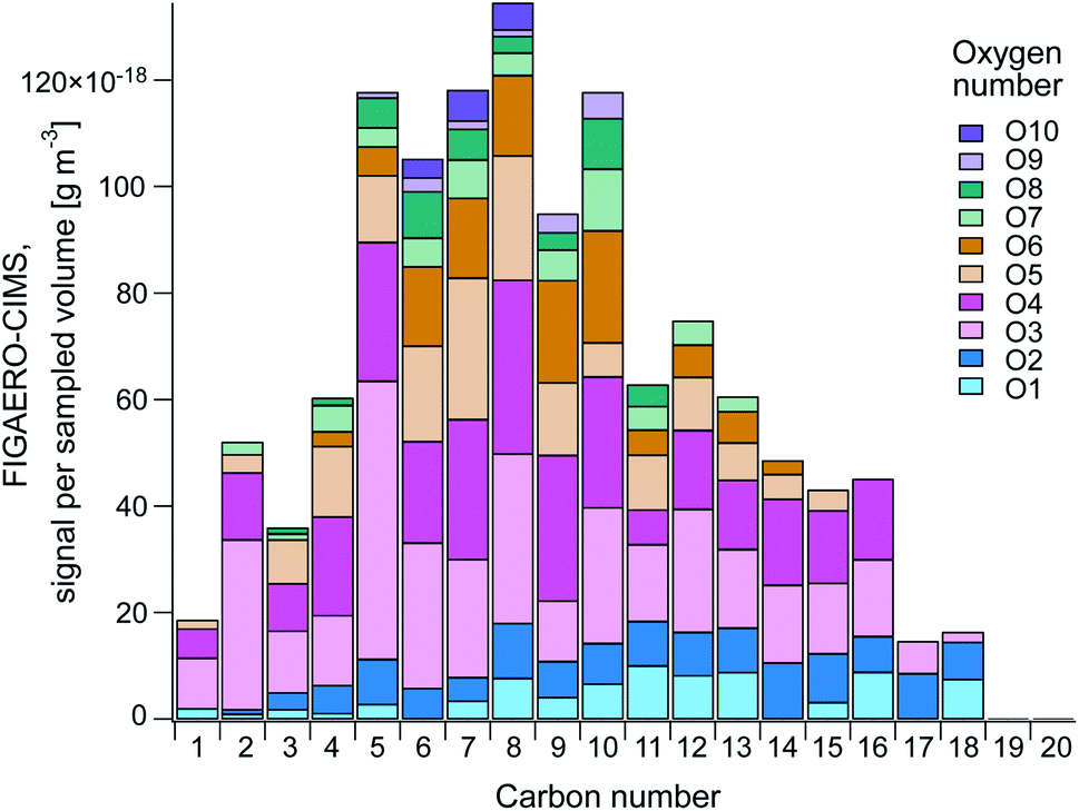

Fig. 6 Aggregated CHO, CHON, CHONS and CHOS median signal of all samples (F1–F13) by carbon number (C1–C20) and coloured by oxygen number (O1–O10). The figure shows the distribution of carbon and oxygen atoms in the detected compounds.

Fig. 6 shows that the largest signal contribution was from C5-10 compounds, where O3–4 compounds and to some extent O5–6 compounds were generally dominating. C1–4 compounds contained mainly 3–4 oxygen atoms, whereas the relative contribution of O1–2 increased at higher carbon numbers (C11–18). The compounds with a high carbon and low oxygen number all belonged to the CHO and CHON categories, and their molecular formulas indicate different fatty acids, implying a primary SSA origin. Fatty acids in the range C8–24 have previously been found in SML samples from the central Arctic Ocean through analysis with ultrahigh-performance liquid chromatography/travelling-wave ion mobility/time-of-flight mass spectrometry (UHPLC/TWIMS/TOFMS) by Mashayekhy Rad et al.⁹⁰ Whereas they found the largest contribution to be from hexadecanoic (C₁₆H₃₂O₂) and octadecanoic acids (C₁₈H₃₆O₂), our results show that the highest signal came from C₁₅H₂₈O₂ and C₁₁H₂₂O₂ and that hexadecanoic and octadecanoic acids were not above LOD. As the analytical techniques are different, they are probably sensitive to different compounds. This implies that the FIGAERO-CIMS can complement other analytical techniques to provide extended knowledge about the Arctic environment. However, it could also be an indication of that the fatty acids dominating the SML are not being emitted to the atmosphere to the same extent as other fatty acids.

The largest number and highest combined signal intensity (66%) was from CHO compounds, which also had the highest average carbon number (8.96), followed by CHON (30.0% and 8.58). Only 4 and 15 compounds remained in the CHONS and CHOS categories, respectively. Such small numbers do not allow for statistical analyses, however, the CHOS category did not have any contribution of compounds >C8 and 66.1% was made up by C1–2 compounds. The small carbon number together with the highest O : C ratio (1.34) indicates a large contribution of DMS oxidation products to this category.⁹¹ The high O : C ratio also implies a secondary origin and a higher degree of aging (oxidation) of the aerosols in this category.

In Fig. 7, we have taken the compound groups from Fig. 6 and aggregated them further to compound groups with 1–2, 3–4, 5–6, and >6 oxygen atoms. In Fig. 7 we show the relative contributions of the summed signal of all compounds in these respective groups per filter sample. Overall, for all filter samples, compounds with 3–4 oxygen atoms dominated the signal (51–85%), followed by compounds with 5–6 oxygen atoms (9–38%), and compounds with 1–2 oxygen atoms (6–26%). Compounds with >6 oxygen atoms made up 0–10% of the total signal. As the samples were collected in different environments (pack ice, transit and MIZ), and Fig. 5 indicates more time spent over the ocean compared to the pack ice for the samples collected later during the measurement period (F8–F13), one would expect the degree of oxygenation (as a measure of aerosol aging processes) to vary between the different samples. Clear differences between samples from ice floe, transit, or MIZ are however not distinguishable, indicating that the time resolution of data presented here is not necessarily sufficient to clearly separate temporally varying influence of different regional aerosol sources purely based on molecular composition.

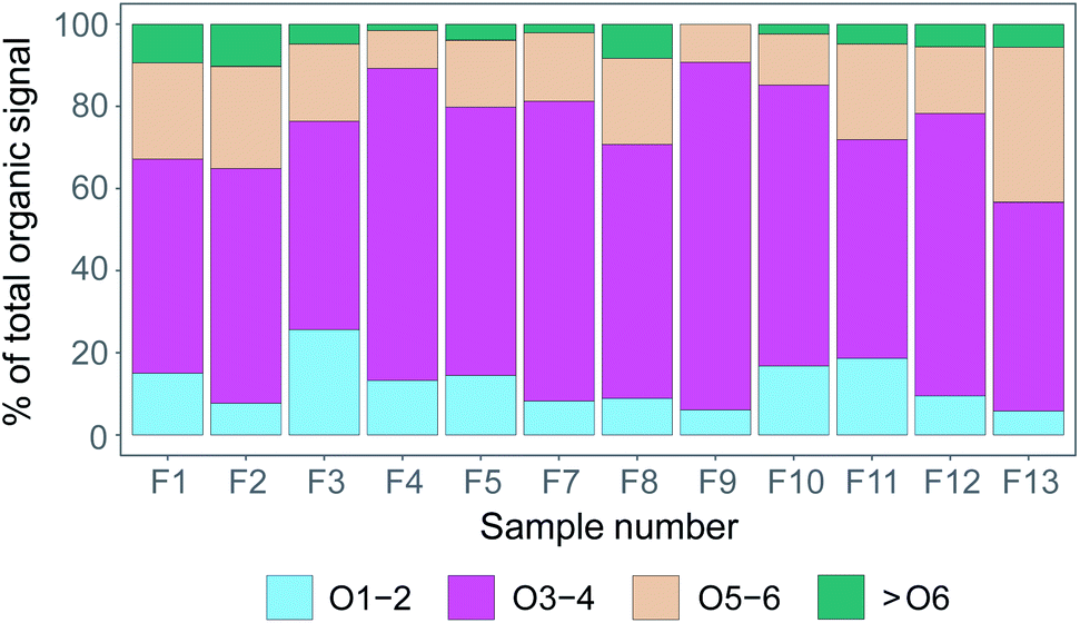Fig. 7 Percentage of the sample signal from organic compounds including 1–2 oxygen atoms (O1–2), 3–4 (O3–4), 5–6 (O5–6) and more than 6 oxygen atoms (>O6).

3.4 DMS oxidation products

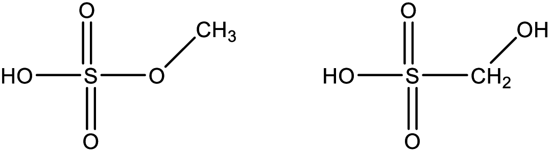
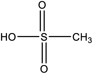
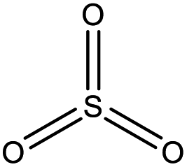
Among the compounds clearly identified in the samples analysed by FIGAERO-CIMS are the inorganic molecules sulfuric acid (SA; H₂SO₄), sulfur trioxide (SO₃; probably a fragmentation product of SA), and the organic methanesulfonic acid (MSA, CH₃SO₃H) and monomethyl sulfate and/or hydroxymethanesulfonic acid (CH₃SO₄H), as the FIGAERO-CIMS cannot distinguish compounds with different molecular structures but with the same molecular formula (Table 2). These compounds are known as atmospheric oxidation products of DMS.^92,93 H₂O(SO₃)₂, a dimer of SA, was also detected in some of the samples. As this was the first time the FIGAERO-CIMS was used for high Arctic aerosol samples, a comparison of measured SA and MSA to concurrent techniques onboard Oden is presented in Fig. S8.† Detection of methanesulfinic acid (MSIA; CH₃SO₂H) and sulfur dioxide (SO₂) would also be indicative of DMS oxidation, but these compounds were not identified in the samples since their signal could not be separated from that of SO₃ and the isotope of nitric acid (HNO₃), respectively, in the raw data. No traces of HPMTF, which has previously been reported in air samples over productive marine areas by Veres et al.,⁴² were found in the aerosol samples. As shown in their study, measured HPMTF gas-phase concentrations were relatively low in the polar regions within the MBL, and it is not clear if this compound eventually partitions into the particle phase or not.

Table 2 Oxidation products of DMS identified in the aerosol samples by FIGAERO-CIMS

Compound name	Molecular formula	Molecular structure
Disulfuric acid	H2O(SO3)2
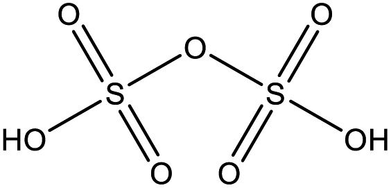
Sulfuric acid (SA)	H2SO4
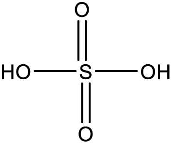
Monomethyl sulfate/hydroxymethanesulfonic acid	CH3SO4H
Methanesulfonic acid (MSA)	CH3SO3H
Sulfur trioxide	SO3

---

3.5 DMS oxidation products in gas- and particle-phase

Previous studies⁹⁴ have shown that approximately 10% of the DMS emitted into the Arctic boundary layer originates from the central Arctic Ocean (<2% from the pack ice area, i.e. open leads, cracks and melt ponds) and 90% from the surrounding seas (the Greenland, Barents and Kara Seas). The DMS oxidation products we measured in the aerosol samples in the pack ice were therefore likely produced to a large extent during advection over the ice from the surrounding seas. By comparing the concentrations of DMS and its oxidation products in the gas- and particle phase at various distances from the source region, conclusions can be drawn both on source regions as well as the influence of atmospheric transport on the particle chemical composition.

Fig. 8a shows a time series of DMS, SA and MSA in the gas phase, and Fig. 8b the time series of particulate SA, SO₃, MSA and CH₃SO₄H. Overall it can be seen that the gas-phase compounds exhibit elevated concentrations towards the end of the measurement period when the ship approached the MIZ, whereas the compounds in the particle phase follow the general pattern of particle mass concentrations as shown in Fig. 3.

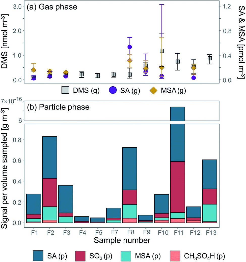Fig. 8 DMS and its oxidation products (a) sulfuric acid (SA) and methanesulfonic acid (MSA) in the gas phase (g) (median value of the same sampling periods as the aerosol samples F1–F13) and (b) particle-phase (p) SA, MSA, sulfur trioxide (SO₃) and monomethyl sulfate/hydroxymethane sulfonic acid (CH₃SO₄H) (see Table 2). The error bars in (a) represent the 95^th and 5^th percentiles.

Measured DMS (g) concentrations during the measurement period ranged between 0.055 and 2.0 nmol m⁻³, with a median of 0.68 nmol m⁻³. The highest concentration (2.0 nmol m⁻³) was measured on 17 September at 04:22 and the lowest concentration (0.055 nmol m⁻³) on 14 September at 15:55. A comparison to measured atmospheric DMS concentrations during previous expeditions with I/B Oden can be found in Table S5.† Ambient SA (g) ranged between 5.87 × 10⁻⁶ (11 September 15:20–16:30) and 1.48 × 10⁻³ nmol m⁻³ (17 September 12:20) with a median of 6.62 × 10⁻⁵ nmol m⁻³, and MSA (g) between 4.33 × 10⁻⁵ (17 September 00:00) and 0.801 nmol m⁻³ (17 September 12:20) with a median of 1.81 × 10⁻⁴ nmol m⁻³. MSA (g) should in theory not be influenced by pollution, since its only source is DMS, which is emitted from the ocean. However, it follows the same pattern as SA (g), which is assumed to have been influenced by ship contamination when the icebreaker was in transit (F8–F11, Table 1). It is possible that gaseous and particulate pollutants in the ship exhaust impact MSA production and partitioning. Therefore, measured MSA (p) and SA (p) may also co-vary in the contaminated samples.

The highest signal of DMS oxidation products (p) was found on 18 September (F11), followed by 12 September (F2), 15 September (F8) and 19 September (F13). However, since SA and SO₃ can be produced by not only marine sources but also e.g. ship exhaust, the high levels of these compounds in F11 are probably biased by contamination from the ship (see Table 1). F1–F5 were pristine samples without influence of contamination, and these inorganic signals are therefore assumed to originate from natural sources. The highest signal of organic DMS oxidation products (p) was found on 15 September (F8) and 19 September (F13), with elevated signals also found around 12 (F3) and 17 September (F10). SA (p) dominated in all aerosol samples, while the median concentration of SA (g) was slightly lower than MSA (g). These observational results could add to previous model findings, where SA was found to partition to a higher degree into the particle phase compared to MSA.⁹⁵ However, a larger data set would be needed to be able to state this for sure.

DMS has a turnover time over the pack ice of τ ≈ 3 days, i.e. after 3 days over the pack ice 5–10% of the amount remains.^31,96 This means that the air masses that had spent the last 5 days over the pack ice (11 September–approximately 14 September) should contain less DMS compared to the second part of the measurement period (15–19 September). This is confirmed by the back trajectory analysis in Fig. 5, although current oxidant levels and meteorological conditions along the trajectory will also play a role. However, this interpretation is complicated by the fact that (a) the ship was simultaneously progressing southward through the pack ice or was situated in the MIZ and (b) the change of ship position coincided with the influx of air masses with higher DMS levels. Sample F12 and F13 were in the MIZ, where the surrounding ocean was a local DMS source and DMS did not need to be transported to be measured. Similar results of elevated DMS levels while approaching the ice edge were obtained during the ASCOS 2008 ³⁸ and AOE-96 ³²) expeditions.

A correlation of DMS (g) with SA (g, p) and MSA (g, p) is not evident from Fig. 8. DMS is produced far from the inner pack ice area, and as it is advected over the ice it undergoes oxidation. The oxidation products can however be oxidised further (age), which decreases the degree of linearity between DMS and its oxidation products with time. These results are in line with earlier studies in the central Arctic Ocean³⁸ and Antarctica,^97,98 which have also not been able to find a clear correlation between DMS and its oxidation products in aerosols over the ice.

4 Conclusions

We measured the molecular composition of semi-volatile aerosol components using FIGAERO-CIMS (Filter Inlet for Gases and AEROsols coupled to a Chemical Ionization Mass Spectrometer) analysis of filter samples collected on 11–19 September 2018 during the MOCCHA campaign (Microbiology-Ocean-Cloud-Coupling in the High Arctic) in the pack ice close to the North Pole (88.6°N, 45.0°E to 82.3°N, 20.1°E).

Our analysis shows that oxygenated organic and sulfur-containing compounds were abundant in the aerosol samples, including oxidation products of dimethyl sulfide (DMS) such as sulfuric acid (H₂SO₄), methanesulfonic acid (MSA; CH₃SO₃H) and monomethyl sulfate/hydroxymethane sulfonic acid (CH₃SO₄H). Organic compounds consisting of carbon (C), hydrogen (H) and oxygen (O) atoms (CHO) were most abundant (had the highest combined signal) and exhibited a wide range of molecular composition (1–18 carbon atoms with varying numbers of oxygen atoms (1–10) and elemental O : C ratios). We also identified organic compounds containing nitrogen (N) (CHON) and/or sulfur (S) (CHOS, CHONS) as well as halogens. Compared to CHO and CHON compounds, the molecules in the CHOS category in general exhibited fewer carbon atoms and relatively high O : C ratios. As molecules with 1 and 2 carbon atoms dominated this category, it can be assumed that a large fraction of the CHOS compounds were derived from DMS oxidation. More complex compounds with a larger number of carbons and a low O : C ratio (1–2 oxygen atoms), the molecular composition of which indicates fatty acids and other lipids, were also detected, revealing potential influence from primary organic sea spray aerosols. As fatty acids are known to be surface active depending on their alkyl chain length and polarity, our information about their molecular composition can help estimate their effects on e.g. cloud formation and cloud droplet stability.

The time evolution of the integrated filter signals from FIGAERO-CIMS showed qualitatively good agreement with total organic (Org) and sulfate (SO₄²⁻) particulate concentrations measured by an AMS and total submicron (D_p <1 μm) mass concentrations derived from particle size distribution measurements. For periods when total submicron particle mass was clearly higher than AMS Org and SO₄²⁻, a clear shift in particle size distributions to larger particles could be observed. These periods further appeared to coincide with higher wind speeds, suggesting that these samples had a more pronounced influence of larger and locally produced primary SSA particles.

The comparison of the time series of DMS oxidation products in the gas- and particle phase reveals an interesting pattern: for the period in the beginning of the measurements, when the ship was moored to an ice floe and air masses had spent time over the pack ice before arriving at the ship, the elevated particle concentrations were not reflected in the gas-phase concentrations. For the period in the end of the filter sampling period, when the ship was closer to the MIZ, not only elevated particle-, but also higher gas-phase concentrations were observed. However, the average molecular composition of particles measured by FIGAERO-CIMS did not show significant differences between the two locations, indicating that higher gaseous concentrations measured close to the MIZ are not immediately influencing particle composition.

Our study shows that, (1) the submicron aerosols within the central Arctic boundary layer during late summer have a large contribution from organic and sulfur-containing molecules with a wide range of carbon and oxygen numbers, and (2) that gas- and particle-phase chemical composition of organic sulfur compounds in the central Arctic did not co-vary in time. Future studies might detect a more direct relationship as a result of increased particle fluxes and less pack ice, as the sea ice retreat continues northward and the Arctic Ocean is transformed from a polar to a more marine area in the coming decades.

This is the first time that the chemical composition of aerosols in the central Arctic was measured using FIGAERO-CIMS. Similar research has previously been conducted in the Arctic with results comparable to ours using other techniques. However, most of these measurements were conducted in the lower Arctic and on land.^35–37 These studies, along with that presented by Chang et al.³⁸ from the central Arctic Ocean, have provided information on functional groups present while our study also provides information on the molecular composition of the aerosol. As such, this study suggests that the FIGAERO-CIMS can provide new insights into the aerosol chemical composition in the Arctic as well as other pristine environments.

Future work with FIGAERO-CIMS in the central Arctic Ocean should include gas-phase measurements with the FIGAERO for direct comparison between gas- and particle-phase chemical composition. For particle-phase measurements, larger sample loads should be aimed for either by increasing the sampling time or sampling flow, since aerosol concentrations in the Arctic are much lower than in other regions where FIGAERO-CIMS has been more commonly used (e.g. urban areas). The sampling time/flow and sample load should also be optimised to not lose time resolution. Another advantage would be to simultaneously use several CIMS setups with different reagent ions (e.g. iodide, nitrate and ammonium), to gain a more complete picture of the semi-volatile compounds present in Arctic aerosol.

Conflicts of interest

There are no conflicts to declare.

Acknowledgements

We thank Heini Wernli (ETH Zürich, Switzerland) for providing the calculated back trajectory data, Dominic Heslin-Rees for sharing the trajectory averaging script and Aitor Aldama Campino for help with modifications, map figures and document formatting. We thank the Bolin Centre for Climate Research data base for providing the meteorological data and John Prytherch for help with data interpretation. Sophie Haslett is thanked for extensive help with Tofware, programming in Igor and for sharing the O : C script, and together with Yvette Gramlich and Cheng Wu for support with sample and data analysis. Luisa Ickes and Joachim Dillner are thanked for their work with the inlet pollution control system, Nils Walberg and Joachim Dillner for the inlet setup and Emmy Nilsson for quality assurance of the DMS samples. We are grateful to Lise Lotte Sørensen, Kasper Kristensen and Linda Megner for valuable input on the research and manuscript. The Swedish Polar Research (SPRS) provided access to the icebreaker Oden and logistical support. We are grateful to the SPRS logistical staff and to Oden's Captain Mattias Peterson and his crew. This work was supported by the Swedish Research Council (grant no. 2016-03518, 2018-04255 and 2016-05100), the Swedish Research Council for Sustainable Development FORMAS (grant no. 2015-00748, 2017-00567), the Knut and Alice Wallenberg Foundation (ACAS project, grant no. 2016.0024 and WAF project CLOUDFORM, grant no. 2017.0165), the Swiss National Science Foundation (grant no. 200021_169090), the Swiss Polar Institute, the FORCeS project and the Bolin Centre for Climate Research at Stockholm University. Julia Schmale holds the Ingvar Kamprad Chair for Extreme Environments research.

Notes and references

1. K. E. Taylor, R. J. Stouffer and G. A. Meehl, Bull. Am. Meteorol. Soc., 2012, 93, 485–498.
2. H. Pörtner, D. Roberts, V. Masson-Delmotte, P. Zhai, M. Tignor, E. Poloczanska, K. Mintenbeck, M. Nicolai, A. Okem, J. Petzold, B. Rama and N. M. Weyer, IPCC Intergovernmental Panel on Climate Change, Geneva, Switzerland, 2019.
3. P. Brimblecombe, Air composition and chemistry, Cambridge University Press, 1996.
4. M. Jacobson, H.-C. Hansson, K. Noone and R. Charlson, Rev. Geophys., 2000, 38, 267–294.
5. J. H. Seinfeld and S. N. Pandis, Atmospheric chemistry and physics: from air pollution to climate change, John Wiley & Sons, 2016.
6. T. Novakov and J. Penner, Nature, 1993, 365, 823–826.
7. J. A. Curry, Sci. Total Environ., 1995, 160, 777–791.
8. T. Mauritsen, J. Sedlar, M. Tjernström, C. Leck, M. Martin, M. Shupe, S. Sjögren, B. Sierau, P. Persson and I. Brooks, Atmos. Chem. Phys., 2011, 11, 165–173.
9. K. Loewe, A. M. Ekman, M. Paukert, J. Sedlar, M. Tjernström and C. Hoose, Atmos. Chem. Phys., 2017, 17, 6693–6704.
10. R. G. Stevens, K. Loewe, C. Dearden, A. Dimitrelos, A. Possner, G. K. Eirund, T. Raatikainen, A. A. Hill, B. J. Shipway, J. Wilkinson, S. Romakkaniemi, J. Tonttila, A. Laaksonen, H. Korhonen, P. Connolly, U. Lohmann, C. Hoose, A. M. L. Ekman, K. S. Carslaw and P. R. Field, Atmos. Chem. Phys., 2018, 18, 11041–11071.
11. L. M. Russell, S. F. Maria and S. C. Myneni, Geophys. Res. Lett., 2002, 29, 26–31.
12. J. Schmale, P. Zieger and A. M. Ekman, Nat. Clim. Change, 2021, 11, 95–105.
13. K. R. Greenaway, Experiences with Arctic flying weather, Royal Meteorological Society, Canadian Branch, 1950.
14. J. Mitchell, J. Atmos. Terr. Phys., 1957, 17, 195–211.
15. L. Qi, Q. Li, D. K. Henze, H.-L. Tseng and C. He, Atmos. Chem. Phys., 2017, 17, 9697–9716.
16. L. Qi, Q. Li, Y. Li and C. He, Atmos. Chem. Phys., 2017, 17, 1037–1059.
17. J.-W. Xu, R. V. Martin, A. Morrow, S. Sharma, L. Huang, W. R. Leaitch, J. Burkart, H. Schulz, M. Zanatta, M. D. Willis, D. K. Henze, C. J. Lee, A. B. Herber and J. P. D. Abbatt, Atmos. Chem. Phys., 2017, 17, 11971–11989.
18. P. Quinn, G. Shaw, E. Andrews, E. Dutton, T. Ruoho-Airola and S. Gong, Tellus B, 2007, 59, 99–114.
19. K. S. Law and A. Stohl, Science, 2007, 315, 1537–1540.
20. P. Tunved, J. Ström and R. Krejci, Atmos. Chem. Phys., 2013, 13, 3643–3660.
21. E. Freud, R. Krejci, P. Tunved, R. Leaitch, Q. T. Nguyen, A. Massling, H. Skov and L. Barrie, Atmos. Chem. Phys., 2017, 17, 8101–8128.
22. M. Karl, C. Leck, F. Mashayekhy Rad, A. Bäcklund, S. Lopez-Aparicio and J. Heintzenberg, Tellus B, 2019, 71, 1613143.
23. C. Leck, E. K. Bigg, D. S. Covert, J. Heintzenberg, W. Maenhaut, E. D. Nilsson and A. Wiedensohler, Tellus B, 1996, 48, 136–155.
24. C. Leck, E. D. Nilsson, E. K. Bigg and L. Bäcklin, J. Geophys. Res.: Atmos., 2001, 106, 32051–32067.
25. C. Leck, M. Tjernström, P. Matrai, E. Swietlicki and K. Bigg, Eos Trans. AGU, 2004, 85, 25–32.
26. M. Tjernström, Boundary-Layer Meteorology, 2005, 117, 5–36.
27. M. Tjernström, C. Leck, C. E. Birch, J. W. Bottenheim, B. J. Brooks, I. M. Brooks, L. Bäcklin, R. Y.-W. Chang, G. de Leeuw, L. Di Liberto, S. de la Rosa, E. Granath, M. Graus, A. Hansel, J. Heintzenberg, A. Held, A. Hind, P. Johnston, J. Knulst, M. Martin, P. A. Matrai, T. Mauritsen, M. Müller, S. J. Norris, M. V. Orellana, D. A. Orsini, J. Paatero, P. O. G. Persson, Q. Gao, C. Rauschenberg, Z. Ristovski, J. Sedlar, M. D. Shupe, B. Sierau, A. Sirevaag, S. Sjogren, O. Stetzer, E. Swietlicki, M. Szczodrak, P. Vaattovaara, N. Wahlberg, M. Westberg and C. R. Wheeler, Atmos. Chem. Phys., 2014, 14, 2823–2869.
28. A. N. Schwier, C. Rose, E. Asmi, A. M. Ebling, W. M. Landing, S. Marro, M.-L. Pedrotti, A. Sallon, F. Iuculano, S. Agusti, A. Tsiola, P. Pitta, J. Louis, C. Guieu, F. Gazeau and K. Sellegri, Atmos. Chem. Phys., 2015, 15, 7961–7976.
29. L. T. Cravigan, M. D. Mallet, P. Vaattovaara, M. J. Harvey, C. S. Law, R. L. Modini, L. M. Russell, E. Stelcer, D. D. Cohen, G. Olsen, K. Safi, T. J. Burrell and Z. Ristovski, Atmos. Chem. Phys., 2020, 20, 7955–7977.
30. R. L. Modini, B. Harris and Z. Ristovski, Atmos. Chem. Phys., 2010, 10, 2867–2877.
31. C. Leck and C. Persson, Tellus B, 1996, 48, 272–299.
32. C. Leck, M. Norman, E. K. Bigg and R. Hillamo, J. Geophys. Res.: Atmos., 2002, 107, AAC-1.
33. E. K. Bigg, C. Leck and L. Tranvik, Mar. Chem., 2004, 91, 131–141.
34. M. V. Orellana, P. A. Matrai, C. Leck, C. D. Rauschenberg, A. M. Lee and E. Coz, Proc. Natl. Acad. Sci., 2011, 108, 13612–13617.
35. P. M. Shaw, L. M. Russell, A. Jefferson and P. K. Quinn, Geophys. Res. Lett., 2010, 37, L10803.
36. M. D. Willis, F. Köllner, J. Burkart, H. Bozem, J. L. Thomas, J. Schneider, A. A. Aliabadi, P. M. Hoor, H. Schulz, A. B. Herber, W. R. Leaitch and J. P. D. Abbatt, Geophys. Res. Lett., 2017, 44, 6460–6470.
37. W. R. Leaitch, L. M. Russell, J. Liu, F. Kolonjari, D. Toom, L. Huang, S. Sharma, A. Chivulescu, D. Veber and W. Zhang, Atmos. Chem. Phys., 2018, 18, 3269–3287.
38. R. Y.-W. Chang, C. Leck, M. Graus, M. Müller, J. Paatero, J. F. Burkhart, A. Stohl, L. H. Orr, K. Hayden, S.-M. Li, A. Hansel, M. Tjernström, W. R. Leaitch and J. P. D. Abbatt, Atmos. Chem. Phys., 2011, 11, 10619–10636.
39. M. Gourdal, O. Crabeck, M. Lizotte, V. Galindo, M. Gosselin, M. Babin, M. Scarratt and M. Levasseur, Elementa, 2019, 7, 33.
40. M. Kulmala, L. Pirjola and J. M. Mäkelä, Nature, 2000, 404, 66–69.
41. V.-M. Kerminen and C. Leck, J. Geophys. Res.: Atmos., 2001, 106, 32087–32099.
42. P. R. Veres, J. A. Neuman, T. H. Bertram, E. Assaf, G. M. Wolfe, C. J. Williamson, B. Weinzierl, S. Tilmes, C. R. Thompson, A. B. Thames, J. C. Schroder, A. Saiz-Lopez, A. W. Rollins, J. M. Roberts, D. Price, J. Peischl, B. A. Nault, K. H. Møller, D. O. Miller, S. Meinardi, Q. Li, J.-F. Lamarque, A. Kupc, H. G. Kjaergaard, D. Kinnison, J. L. Jimenez, C. M. Jernigan, R. S. Hornbrook, A. Hills, M. Dollner, D. A. Day, C. A. Cuevas, P. Campuzano-Jost, J. Burkholder, T. P. Bui, W. H. Brune, S. S. Brown, C. A. Brock, I. Bourgeois, D. R. Blake, E. C. Apel and T. B. Ryerson, Proc. Natl. Acad. Sci., 2020, 117, 4505–4510.
43. R. J. Charlson, J. E. Lovelock, M. O. Andreae and S. G. Warren, Nature, 1987, 326, 655–661.
44. G. P. Ayers and J. M. Cainey, Environ. Chem., 2008, 4, 366–374.
45. T. K. Green and A. D. Hatton, Oceanogr. Mar. Biol., 2014, 52, 315–336.
46. C. Leck and E. K. Bigg, Environ. Chem., 2007, 4, 400–403.
47. P. K. Quinn and T. S. Bates, Nature, 2011, 480, 51–56.
48. P. K. Quinn, T. L. Miller, T. S. Bates, J. A. Ogren, E. Andrews and G. E. Shaw, J. Geophys. Res.: Atmos., 2002, 107, AAC 8-1–AAC 8-15.
49. W. R. Leaitch, S. Sharma, L. Huang, D. Toom-Sauntry, A. Chivulescu, A. M. Macdonald, K. von Salzen, J. R. Pierce, A. K. Bertram, J. C. Schroder, N. C. Shantz, R. Y.-W. Chang and A.-L. Norman, Elementa, 2013, 1, 000017.
50. M. D. Willis, J. Burkart, J. L. Thomas, F. Köllner, J. Schneider, H. Bozem, P. M. Hoor, A. A. Aliabadi, H. Schulz, A. B. Herber, W. R. Leaitch and J. P. D. Abbatt, Atmos. Chem. Phys., 2016, 16, 7663–7679.
51. J. P. D. Abbatt, W. R. Leaitch, A. A. Aliabadi, A. K. Bertram, J.-P. Blanchet, A. Boivin-Rioux, H. Bozem, J. Burkart, R. Y. W. Chang, J. Charette, J. P. Chaubey, R. J. Christensen, A. Cirisan, D. B. Collins, B. Croft, J. Dionne, G. J. Evans, C. G. Fletcher, M. Galí, R. Ghahremaninezhad, E. Girard, W. Gong, M. Gosselin, M. Gourdal, S. J. Hanna, H. Hayashida, A. B. Herber, S. Hesaraki, P. Hoor, L. Huang, R. Hussherr, V. E. Irish, S. A. Keita, J. K. Kodros, F. Köllner, F. Kolonjari, D. Kunkel, L. A. Ladino, K. Law, M. Levasseur, Q. Libois, J. Liggio, M. Lizotte, K. M. Macdonald, R. Mahmood, R. V. Martin, R. H. Mason, L. A. Miller, A. Moravek, E. Mortenson, E. L. Mungall, J. G. Murphy, M. Namazi, A.-L. Norman, N. T. O'Neill, J. R. Pierce, L. M. Russell, J. Schneider, H. Schulz, S. Sharma, M. Si, R. M. Staebler, N. S. Steiner, J. L. Thomas, K. von Salzen, J. J. B. Wentzell, M. D. Willis, G. R. Wentworth, J.-W. Xu and J. D. Yakobi-Hancock, Atmos. Chem. Phys., 2019, 19, 2527–2560.
52. P. Fu, K. Kawamura, J. Chen, B. Charrìère and R. Sempere, Biogeosciences, 2013, 10, 653–667.
53. E. L. Mungall, J. P. D. Abbatt, J. J. B. Wentzell, A. K. Y. Lee, J. L. Thomas, M. Blais, M. Gosselin, L. A. Miller, T. Papakyriakou, M. D. Willis and J. Liggio, Proc. Natl. Acad. Sci., 2017, 114, 6203–6208.
54. E. L. Mungall, J. P. D. Abbatt, J. J. B. Wentzell, G. R. Wentworth, J. G. Murphy, D. Kunkel, E. Gute, D. W. Tarasick, S. Sharma, C. J. Cox, T. Uttal and J. Liggio, Atmos. Chem. Phys., 2018, 18, 10237–10254.
55. J. H. Kroll and J. H. Seinfeld, Atmos. Environ., 2008, 42, 3593–3624.
56. Y. Li, U. Pöschl and M. Shiraiwa, Atmos. Chem. Phys., 2016, 16, 3327–3344.
57. M. D. Petters and S. M. Kreidenweis, Atmos. Chem. Phys., 2007, 7, 1961–1971.
58. N. M. Donahue, J. H. Kroll, S. N. Pandis and A. L. Robinson, Atmos. Chem. Phys., 2012, 12, 615–634.
59. C. Mohr, J. A. Thornton, A. Heitto, F. D. Lopez-Hilfiker, A. Lutz, I. Riipinen, J. Hong, N. M. Donahue, M. Hallquist, T. Petäjä, M. Kulmala and T. Yli-Juuti, Nat. Commun., 2019, 10, 4442.
60. F. D. Lopez-Hilfiker, C. Mohr, M. Ehn, F. Rubach, E. Kleist, J. Wildt, T. F. Mentel, A. Lutz, M. Hallquist, D. Worsnop and J. A. Thornton, Atmos. Meas. Tech., 2014, 7, 983–1001.
61. C. Leck, P. Matrai, A.-M. Perttu and K. Gårdfeldt, Expedition report: SWEDARTIC Arctic Ocean 2018, 2019.
62. N. A. Rayner, D. E. Parker, E. B. Horton, C. K. Folland, L. V. Alexander, D. P. Rowell, E. C. Kent and A. Kaplan, J. Geophys. Res.: Atmos., 2003, 108, 4407.
63. S.-L. Von der Weiden, F. Drewnick and S. Borrmann, Atmos. Meas. Tech., 2009, 2, 479–494.
64. W. Huang, H. Saathoff, X. Shen, R. Ramisetty, T. Leisner and C. Mohr, Atmos. Chem. Phys., 2019, 19, 11687–11700.
65. B. B. Rasmussen, Q. T. Nguyen, K. Kristensen, L. S. Nielsen and M. Bilde, J. Aerosol Sci., 2017, 107, 134–141.
66. B. H. Lee, F. D. Lopez-Hilfiker, C. Mohr, T. Kurtén, D. R. Worsnop and J. A. Thornton, Environ. Sci. Technol., 2014, 48, 6309–6317.
67. M. Riva, P. Rantala, J. E. Krechmer, O. Peräkylä, Y. Zhang, L. Heikkinen, O. Garmash, C. Yan, M. Kulmala, D. Worsnop and M. Ehn, Atmos. Meas. Tech., 2019, 12, 2403–2421.
68. S. Iyer, F. Lopez-Hilfiker, B. H. Lee, J. A. Thornton and T. Kurtén, J. Phys. Chem. A, 2016, 120, 576–587.
69. S. L. Thompson, R. L. N. Yatavelli, H. Stark, J. R. Kimmel, J. E. Krechmer, D. A. Day, W. Hu, G. Isaacman-VanWertz, L. Yee, A. H. Goldstein, M. A. H. Khan, R. Holzinger, N. Kreisberg, F. D. Lopez-Hilfiker, C. Mohr, J. A. Thornton, J. T. Jayne, M. Canagaratna, D. R. Worsnop and J. L. Jimenez, Aerosol Sci. Technol., 2017, 51, 30–56.
70. P. F. DeCarlo, J. R. Kimmel, A. Trimborn, M. J. Northway, J. T. Jayne, A. C. Aiken, M. Gonin, K. Fuhrer, T. Horvath, K. S. Docherty, D. R. Worsnop and J. L. Jimenez, Anal. Chem., 2006, 78, 8281–8289.
71. M. Canagaratna, J. Jayne, J. Jimenez, J. Allan, M. Alfarra, Q. Zhang, T. Onasch, F. Drewnick, H. Coe, A. Middlebrook, A. Delia, L. Williams, A. Trimborn, M. Northway, P. DeCarlo, C. Kolb, P. Davidovits and D. Worsnop, Mass Spectrom. Rev., 2007, 26, 185–222.
72. J. Schmale, J. Schneider, E. Nemitz, Y. Tang, U. Dragosits, T. Blackall, P. Trathan, G. Phillips, M. Sutton and C. Braban, Atmos. Chem. Phys., 2013, 13, 8669–8694.
73. S. Nakao, P. Tang, X. Tang, C. H. Clark, L. Qi, E. Seo, A. Asa-Awuku and D. Cocker III, Atmos. Environ., 2013, 68, 273–277.
74. F. Kasten, J. Appl. Meteorol., 1968, 7, 944–947.
75. A. Petzold and M. Schönlinner, J. Aerosol Sci., 2004, 35, 421–441.
76. T. Müller, J. S. Henzing, G. de Leeuw, A. Wiedensohler, A. Alastuey, H. Angelov, M. Bizjak, M. Collaud Coen, J. E. Engström, C. Gruening, R. Hillamo, A. Hoffer, K. Imre, P. Ivanow, G. Jennings, J. Y. Sun, N. Kalivitis, H. Karlsson, M. Komppula, P. Laj, S.-M. Li, C. Lunder, A. Marinoni, S. Martins dos Santos, M. Moerman, A. Nowak, J. A. Ogren, A. Petzold, J. M. Pichon, S. Rodriquez, S. Sharma, P. J. Sheridan, K. Teinilä, T. Tuch, M. Viana, A. Virkkula, E. Weingartner, R. Wilhelm and Y. Q. Wang, Atmos. Meas. Tech., 2011, 4, 245–268.
77. C. Persson and C. Leck, Anal. Chem., 1994, 66, 983–987.
78. F. Eisele and D. Tanner, J. Geophys. Res.: Atmos., 1993, 98, 9001–9010.
79. T. Jokinen, M. Sipilä, H. Junninen, M. Ehn, G. Lönn, J. Hakala, T. Petäjä, R. L. Mauldin III, M. Kulmala and D. R. Worsnop, Atmos. Chem. Phys., 2012, 12, 4117–4125.
80. A. Baccarini, L. Karlsson, J. Dommen, P. Duplessis, J. Vüllers, I. M. Brooks, A. Saiz-Lopez, M. Salter, M. Tjernström, U. Baltensperger, P. Zieger and J. Schmale, Nat. Commun., 2020, 11, 1–11.
81. A. Baccarini, J. Schmale and J. Dommen, Ceilometer backscatter, cloud base height and cloud fraction data from the Arctic Ocean 2018 expedition, 2020, https://bolin.su.se/data/ao2018-aerosol-cims.
82. M. Sprenger and H. Wernli, Geosci. Model Dev., 2015, 8, 2569–2586.
83. J. Prytherch, Weather data from MISU weather station during the Arctic Ocean 2018 expedition, 2020, https://bolin.su.se/data/ao2018-misu-weather-2.
84. J. Prytherch and M. Tjernström, Ceilometer backscatter, cloud base height and cloud fraction data from the Arctic Ocean 2018 expedition, 2020, https://bolin.su.se/data/ao2018-ceilometer-2.
85. E. D. Nilsson and E. K. Bigg, Tellus B, 1996, 48, 234–253.
86. J. M. Intrieri, C. W. Fairall, M. D. Shupe, P. O. G. Persson, E. L. Andreas, P. S. Guest and R. E. Moritz, J. Geophys. Res.: Oceans, 2002, 107, SHE 13-1–SHE 13-14.
87. J. Vüllers, P. Achtert, I. M. Brooks, M. Tjernström, J. Prytherch, A. Burzik and R. Neely III, Atmos. Chem. Phys., 2021, 21, 289–314.
88. J. Prytherch and M. J. Yelland, Global Biogeochem. Cycles, 2021, 35, e2020GB006633.
89. W. Huang, H. Saathoff, X. Shen, R. Ramisetty, T. Leisner and C. Mohr, Environ. Sci. Technol., 2019, 53, 1165–1174.
90. F. Mashayekhy Rad, C. Leck, L. L. Ilag and U. Nilsson, Rapid Commun. Mass Spectrom., 2018, 32, 942–950.
91. F. Yin, D. Grosjean and J. H. Seinfeld, J. Atmos. Chem., 1990, 11, 309–364.
92. I. Barnes, J. Hjorth and N. Mihalopoulos, Chem. Rev., 2006, 106, 940–975.
93. E. H. Hoffmann, A. Tilgner, R. Schroedner, P. Bräuer, R. Wolke and H. Herrmann, Proc. Natl. Acad. Sci., 2016, 113, 11776–11781.
94. C. Leck and C. Persson, Tellus B, 1996, 48, 156–177.
95. A. L. Hodshire, P. Campuzano-Jost, J. K. Kodros, B. Croft, B. A. Nault, J. C. Schroder, J. L. Jimenez and J. R. Pierce, Atmos. Chem. Phys., 2019, 19, 3137–3160.
96. E. D. Nilsson and C. Leck, Tellus B, 2002, 54, 213–230.
97. H. Berresheim, J. Huey, R. Thorn, F. Eisele, D. Tanner and A. Jefferson, J. Geophys. Res.: Atmos., 1998, 103, 1629–1637.
98. K. A. Read, A. C. Lewis, S. Bauguitte, A. M. Rankin, R. A. Salmon, E. W. Wolff, A. Saiz-Lopez, W. J. Bloss, D. E. Heard, J. D. Lee and J. M. C. Plane, Atmos. Chem. Phys., 2008, 8, 2985–2997.

---

Footnote

† Electronic supplementary information (ESI) available. See DOI: 10.1039/d0ea00023j

---