
 Open Access Article
 This Open Access Article is licensed under a Creative Commons Attribution-Non Commercial 3.0 Unported Licence
Molecular dissociation and proton transfer in aqueous methane solution under an electric field
Giuseppe
Cassone
 *a,
Jiri
Sponer
b and
Franz
Saija
a
*a,
Jiri
Sponer
b and
Franz
Saija
a
aInstitute for Chemical-Physical Processes, National Research Council of Italy (IPCF-CNR), Viale F. Stagno d'Alcontres 37, 98158 Messina, Italy. E-mail: cassone@ipcf.cnr.it
bInstitute of Biophysics of the Czech Academy of Sciences, Královopolska 135, 61265 Brno, Czech Republic
First published on 1st November 2021
Abstract
Methane–water mixtures are ubiquitous in our solar system and they have been the subject of a wide variety of experimental, theoretical, and computational studies aimed at understanding their behaviour under disparate thermodynamic scenarios, up to extreme planetary ice conditions of pressures and temperatures [Lee and Scandolo, Nat. Commun., 2011, 2, 185]. Although it is well known that electric fields, by interacting with condensed matter, can produce a range of catalytic effects which can be similar to those observed when material systems are pressurised, to the best of our knowledge, no quantum-based computational investigations of methane–water mixtures under an electric field have been reported so far. Here we present a study relying upon state-of-the-art ab initio molecular dynamics simulations where a liquid aqueous methane solution is exposed to strong oriented static and homogeneous electric fields. It turns out that a series of field-induced effects on the dipoles, polarisation, and the electronic structure of both methane and water molecules are recorded. Moreover, upon increasing the field strength, increasing fractions of water molecules are not only re-oriented towards the field direction, but are also dissociated by the field, leading to the release of oxonium and hydroxyde ions in the mixture. However, in contrast to what is observed upon pressurisation (∼50 GPa), where the presence of the water counterions triggers methane ionisation and other reactions, methane molecules preserve their integrity up to the strongest field explored (i.e., 0.50 V Å−1). Interestingly, neither the field-induced molecular dissociation of neat water (i.e., 0.30 V Å−1) nor the proton conductivity typical of pure aqueous samples at these field regimes (i.e., 1.3 S cm−1) are affected by the presence of hydrophobic interactions, at least in a methane–water mixture containing a molar fraction of 40% methane.
1 Introduction
Methane–water mixtures are ubiquitous in our solar system. They can compose more than 90% of the condensed-phase layers – which can be either icy or liquids depending on the specific thermodynamic conditions – of Neptune and Uranus.1 Moreover, the middle and inner layers for a long time were thought to be composed of almost fully ionised molecules of methane and water.2 First-principles molecular dynamics simulations, carried out a decade ago and aimed at probing extreme pressure and temperature regimes mimicking the conditions found in the layers of Neptune and Uranus, revealed that molecular dissociations and other chemical reactions arise also at milder pressure and temperature conditions typical of less deep and more superficial layers.3 However, albeit the pioneering character of this seminal Car–Parrinello4 molecular dynamics simulation,3 many unresolved issues persist on the capabilities held by methane–water mixtures in ionising, sustaining correlated proton transfers and more complex chemical reactions. If, on the one hand, only unstable covalent bonds were detected under extreme pressure and temperature regimes, on the other hand, the short duration of those simulations (∼10 ps) did not allow to rule out the possibility that – on longer timescales – carbon atoms could segregate and form, e.g., diamond,3,5–7 a circumstance observed in similar simulations of pure methane under equivalent thermodynamic conditions.8 Conversely, a pivotal result emerged in these pioneering first-principles molecular dynamics simulations related to the clear evidence that the presence of water, along with its own associated counterions formed under pressure and at relatively high temperatures, are capable of significantly modifying the chemistry of an a priori apolar and substantially inert molecule such as methane. Furthermore, once formed, oxonium (H3O)+ and hydroxyde (OH)− ions are directly responsible for the catalysis of methane molecular dissociation already at 50 GPa.3Another well-known strategy for triggering the formation of water counterions in aqueous mixtures, and hence for setting the pH of the solution, is that of employing intense external electric fields.9–13 Generally, indeed, electric fields produce a range of (catalytic) effects by interacting with atoms, molecules, and complex matter, which are very similar to those observed when condensed-phase systems are pressurised.14–19 A pioneering quantum-based computational study by Geissler et al.,20 exploiting Car–Parrinello4 molecular dynamics and transition-path sampling,21 confirmed that water dissociation is an extremely unfavored event from an energetic standpoint and that the autoprotolysis of a water molecule under ambient conditions is induced by rare large fluctuations of the local electric field (on the order of ∼1 V Å−1) generated by the neighbouring water molecules. This striking finding implies that the application of electric fields on liquid aqueous solutions would in principle modify the energetic balance of the dissociation reaction, hence giving rise to the onset of the water counterions, as it has subsequently been proven by the pioneering work reported by Saitta et al.12 The released ionic species, under the action of the applied electrostatic potential gradient, would then separate along chains of H-bonded “water wires” via the Grotthuss mechanism. Many other simulations on proton transfer have been reported22–25 and a recent work based on ab initio molecular dynamics (AIMD) simulations has shown the possibility of realising water ionisation and superionic ice VII in strong external electric fields typical of Venus.26 Furthermore, only during the last year, the impact of nuclear quantum effects (NQEs) on the molecular dissociation and proton transfer phenomena induced by electric fields in liquid water has been addressed13via path-integral AIMD (PI-AIMD)27–32 simulations. All these computational investigations correctly predicted some recent experimental findings proving that in aqueous systems electric fields generated by the solvent are on the order of ∼1.0 V Å−1![[thin space (1/6-em)]](https://www.rsc.org/images/entities/char_2009.gif) 33 and that field strengths of ∼0.3 V Å−1 are ubiquitous in neat liquid water and are ultimately responsible for the solvation state of the proton.34 More importantly, albeit these intensities may appear somewhat extreme, even stronger (i.e., >1.0 V Å−1) are the electric fields spontaneously present at the proximity of natural oxides.35–37
33 and that field strengths of ∼0.3 V Å−1 are ubiquitous in neat liquid water and are ultimately responsible for the solvation state of the proton.34 More importantly, albeit these intensities may appear somewhat extreme, even stronger (i.e., >1.0 V Å−1) are the electric fields spontaneously present at the proximity of natural oxides.35–37
When water is mixed with other polar substances, such as either methanol or ethanol, and it is exposed to the action of intense electric fields, analogies and extremely important differences arise with respect to those exhibited by its components under the same conditions.38–40 If, on the one hand, the presence of water increases the proton conductivity of simple alcohol–water mixtures, on the other, it hinders the typical enhancement of the chemical reactivity induced by electric fields.38,39 In fact, the field-induced multifaceted chemistry leading to the synthesis of, e.g., hydrogen, dimethyl ether, and other species observed in neat methanol and in neat ethanol, completely disappears in samples containing an excess of water,38,39 indicating that the presence of water strongly inhibits the chemical reactivity of simple alcohols. On the other hand, the effects induced by the presence of inert molecules such as methane on the protolysis phenomenon have not been investigated so far. Also, the potential effects due to external fields in distorting the electronic structure of apolar molecules in polar solutions – such as methane in water – are, to the best of our knowledge, unknown. In fact, although many interesting simulations were carried out on methane hydrates exposed to external either static or oscillating fields,41–44 the employment of classical force-field molecular dynamics simulations ruled out the possibility to track both potential field-induced molecular dissociations occurring in methane and water molecules with any modification of the electronic structure of the constituting molecules. In these investigations,41–44 indeed, the main objective was aimed at exploring the effects carried by electromagnetic and purely electric fields on the growth, dissociation, and kinetics of methane clathrate hydrates and the highest field strengths were kept well beneath any field threshold (≤0.2 V Å−1) capable of triggering chemical variations in the systems for the just-explained reasons (i.e., incapability, by construction, of simulating bonds' breaking/reforming via classical force-fields molecular dynamics).
Here we report on the first AIMD simulation of a methane–water mixture exposed to intense static electric fields in order to study (i) the field-induced changes in the electronic structures and dipole moments of methane and water, (ii) the impact of methane in affecting the well-known field-induced proton transfer mechanisms occurring in water, and (iii) the possibility of triggering more complex chemical reactions owing to the known high reactivity acquired by carbon atoms under an electric field, similarly to the effects induced by an increase of the external pressure studied in ref. 3. Incidentally, due to the evidence that the investigated – and even stronger – field intensities are naturally found at the proximity of, e.g., apolar oxides,35–37 these systems may represent the planetary locus where the phenomena described in the current study could take place.
2 Methods
We used the software package CP2K,45,46 based on the Born–Oppenheimer approach, to perform ab initio molecular dynamics (AIMD) simulations of a liquid mixture of methane and water under the action of static and homogeneous electric fields applied along a given direction (corresponding to the z-axis). The implementation of an external field in simulation algorithms based on density functional theory (DFT) can be achieved by exploiting the Modern Theory of Polarisation and Berry's phases47–49 whereas when periodic boundary conditions apply – as in the current investigation – implementation of static fields is executed owing to the seminal work by Umari and Pasquarello.50 The interested reader may refer to ref. 51 for a vast and exhaustive presentation of the most used implementations of electric fields in atomistic simulation codes. Moreover, as for the technical implementation of static electric fields in DFT algorithms, the reader can refer to the following literature studies: ref. 47, 48, 50, 52 and 53. It is worth mentioning within this context that fields applied in DFT-based molecular dynamics simulations should be interpreted as microscopic – local – fields rather than macroscopic. This is due to the way in which electric fields are intrinsically implemented in DFT algorithms and because of the limited size of the simulation boxes typically employed in AIMD simulations. In a nutshell, Umari and Pasquarello50 demonstrated that the functional F = EKS({ψkn}) − ε·P({ψkn}), where EKS is the Kohn–Sham energy functional, ε is the field intensity, and P is the polarization, is exploitable as an energy functional for a variational approach to the finite-field problem as well making, hence, electric fields implementable also in AIMD simulations under periodic boundary conditions.Moreover, simulation boxes employed in AIMD simulations are typically small, rendering the externally applied field conceivable as a local electrostatic gradient. In fact, the here simulated methane–water mixture contained 26 CH4 and 38 H2O molecules (i.e., 244 atoms) arranged in a cubic cell with edge equal to 12.23 Å, so as to reproduce a density of 1.0 g cm−3 at room temperature. The choice of employing this specific molar ratio between methane and water molecules (i.e., 0.4:0.6) was dictated by the need of comparing the catalytic electric-field-induced effects with those observed for the same system in ref. 3 but upon pressurisation. Albeit typical simulations of methane–water mixtures are frequently carried out at high pressure regimes (i.e., at high densities),3 many other investigations adopted the standard water density for a plethora of analyses on the liquid mixture including the spontaneous nucleation of methane hydrates,54 their growth and dissociation,44 and the methane solubility in water,55 just to mention a few. The investigated density in the canonical number, volume, and temperature (NVT) ensemble ensures the complete miscibility of methane in water. In fact, although the poor solubility of methane in water (i.e., x(CH4) = 0.008 mole percent (mol%) at 4 kbar) is known, the external pressure corresponding to the simulated thermodynamic state and as determined by an analytical evaluation of the stress tensor of the simulation box is on average equal to 2.5 GPa. As shown in Fig. 3 of ref. 56, the state identified in our simulation, where x(CH4) = 0.4 and the pressure is equal to 2.5 GPa, lies above the solubility line extrapolated by Henry's law. As anticipated above, in order to minimise nonphysical surface effects, the simulated liquid structure was replicated in all spatial directions by adopting periodic boundary conditions. The intensity of the electric field was gradually increased with a step increment of 0.05 V Å−1 from zero up to a maximum of 0.50 V Å−1. In the zero-field case we performed dynamics of 50 ps whereas for each other value of the field intensity, we ran dynamics of 10 ps, thus accumulating a global simulation time equal to 150 ps whereas a time-step of 0.5 fs has been chosen.
Wavefunctions of the atomic species have been expanded in triple-zeta valence plus polarisation (TZVP) basis sets with Goedecker–Teter–Hutter pseudopotentials using the GPW method.57 A plane-wave cutoff of 400 Ry has been imposed. Exchange and correlation effects were treated with the Becke–Lee–Yang–Parr (BLYP)58 density functional. Moreover, in order to take into account dispersion interactions, we employed the dispersion-corrected version of BLYP (i.e., BLYP-D3).59,60 Adoption of the BLYP-D3 functional has been indicated by the widespread evidence that such a functional, when dispersion corrections are taken into account, offers one of the best adherence with the experimental results related to water among the standard Generalised Gradient Approximation (GGA) functionals.61,62 It is well-known indeed that neglecting dispersion corrections leads to a severely over-structured liquid (see, e.g., ref. 63 and references therein). In order to additionally counteract the over-structuring of the intermolecular interactions typically produced by the GGA XC functionals in H-bonded systems like liquid water, simulations were executed at a temperature of 350 K. Although some recent findings magnified the importance of including Nuclear Quantum Effects (NQEs) in the presence of electric fields,13 the required computational cost and the necessity of performing a Wannier centres64,65 analysis for characterising the molecular dipoles and polarisations led us to abandon this interesting option in the current study. In fact, it is well-known that fluctuations and fictitious vibrations induced by thermostats mimicking NQEs in path-integral AIMD (PI-AIMD) simulations exhibit many critical issues on the electronic properties evaluated by means of the Wannier centres.66,67 This way, the dynamics of nuclei was simulated classically within the NVT ensemble using the Verlet algorithm, whereas canonical sampling has been executed by employing a canonical-sampling-through-velocity-rescaling thermostat68 set at a time constant equal to 20 fs.
3 Results and discussion
Structural correlations in liquids are conveniently visualised by the atomistic radial distribution functions (RDFs). These latter are shown in Fig. 1 for the most relevant atoms shaping the microscopic structure of the methane–water mixture here investigated at ambient conditions and in the zero-field regime.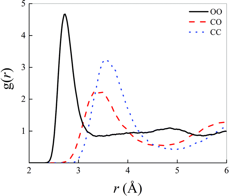 | ||
| Fig. 1 Oxygen–oxygen (black solid curve), carbon–oxygen (red dashed curve), and carbon–carbon (blue dotted curve) radial distribution functions of a methane–water mixture at room temperature and in the zero-field regime. | ||
In particular, the intermolecular water–water correlations typical of neat liquid water are slightly altered by the inclusion of an amount of methane molecules corresponding to a molar fraction equal to 0.4, as depicted by the black solid curve in Fig. 1. In fact, additionally to the partial flattening of the second peak of the oxygen–oxygen (OO) RDF, which indicates damped correlations between a reference water molecule and its second solvation shell, a manifest increase of the height of the first OO RDF maximum is recorded. A peak value larger than 4.5 is, indeed, here detected in a 0.4:0.6 methane–water mixture whereas values around 3.5 are typically reported for the same RDF in bulk liquid water, as determined by means of similar computational techniques.13 By calculating the integral up to the first dip of the OO RDF shown in Fig. 1, a running coordination number equal to 4.58 is obtained, indicating that the presence of hydrophobic interactions – introduced by the presence of methane – somehow compresses the first hydration shell of the aqueous subsystem. Such a value is a ∼13% larger than the typical average number of first-neighbour molecules in pure water (i.e., ∼4.0), quantitatively proving the effectiveness of the qualitative rule “like likes like”. Similarly, correlations magnified by the first peaks of the carbon–oxygen (CO) and carbon–carbon (CC) RDFs are less pronounced in that they exhibit both lower heights and broader widths than the first peak of the OO RDF. Nevertheless, a marked structuring of the intermolecular interactions between water and methane and between methane molecules among each other manifests itself in a net separation between the first two peaks both in the CO and in the CC RDFs displayed in Fig. 1.
When an oriented static and homogeneous external electric field is switched on, some modifications of the OO, CO, and CC RDFs are observed. However, these field-induced changes are quite small, as shown in Fig. 2. In particular, a slight re-entrant effect as a function of the field strength is recorded in the field-induced structural changes on the water subsystem visible in the OO RDF of Fig. 2a. In the low (with respect to the field intensities explored) field regime, an increase of the height of the first peak is accompanied by a simultaneous deepening and shifting towards shorter distances of the OO RDF, indicating a structuring of the H-bond network shaping the connections between water molecules. On the other hand, for field strengths beyond 0.15 V Å−1, this effect partially disappears and the intermolecular structural correlations between the oxygen atoms resemble those recorded in the zero-field regime, with the exception of the first minimum location, as visible in Fig. 2a. As far as the methane–water interactions are concerned, only a slight increase of the height of the first peak is observed upon switching on and increasing the external field intensity, as shown in Fig. 2b. Finally, within the explored range of intensities, quite insensitive to the application of the field are the structural correlations between methane molecules in the 0.4:0.6 methane–water mixture, with the exception of a weak deepening and shifting towards smaller distances of the first dip of the CC RDF, as depicted in Fig. 2c. In other words, the application of static electric fields having strengths up to 0.25 V Å−1 induces a structuring of the water subsystem but does not dramatically alter the intermolecular correlations of the investigated mixture, as it was also found for pure water as simulated with similar techniques.12,13,51,69,70
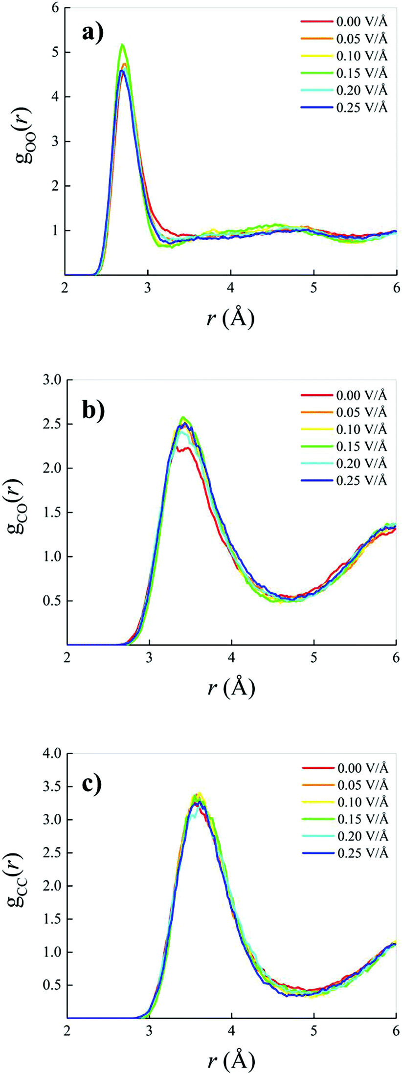 | ||
| Fig. 2 Oxygen–oxygen (a), carbon–oxygen (b), and carbon–carbon (c) radial distribution functions of a methane–water mixture in the zero-field regime (red solid curves) and under increasing electric field strengths (see legends). | ||
Whilst small field-induced changes are also recorded in the intramolecular RDF associated with the behaviour of the carbon–hydrogen (CH) covalent bonds of the methane molecules (Fig. 3a), slightly larger modifications are visible in the oxygen–hydrogen (OH) intramolecular RDF (Fig. 3b), in that the field elongates the distance between the oxygen and the hydrogen atoms within each water molecule, stretching the respective covalent bonds.
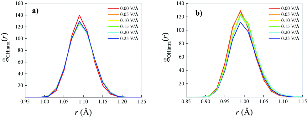 | ||
| Fig. 3 Carbon–hydrogen (a) and oxygen–hydrogen (b) intramolecular radial distribution functions of a methane–water mixture in the zero-field case (red solid curves) and at different electric field intensities (see legends). | ||
On the other hand, net field-induced effects are recorded when characterising the behaviour of the molecular dipole moments constituting the methane–water mixture. Although methane is an apolar molecule in the gas phase, when it is dissolved in a polar liquid such as water at ambient conditions, fractions of methane molecules can transiently assume a small but non-zero dipole moment by interacting with the permanent water dipoles, as shown in Fig. 4a (red solid curve). Technically, this is also likely due, inter alia, to the fact that simulating a methane–water mixture at the standard water density corresponds to a situation in which the system is kept under an external pressure equal to 2.5 GPa, as reported in the Methods section. Besides, upon increasing the intensity of the external oriented electric field, the distributions not only get broader and broader, but also shift their own median towards larger values of the dipole moment magnitude, similarly to the case in which the mixture is subjected to intense external pressures.3 In the most extreme case considered for this specific analysis (i.e., 0.25 V Å−1), the most likely dipole moment magnitude value exhibited by the methane molecules constituting the investigated mixture is ∼0.45 Debye, as shown in Fig. 4a, a value comparable to that recorded under pressures of 15 GPa (i.e., ∼0.5 Debye).3 Such a relatively large dipole moment for an a priori apolar molecule is not only due to the direct presence of the external electrostatic potential gradient, but also to the fact that water molecules are subjected to a similar increase of their dipole moments as well, leading hence to enhanced contributions of the local electric field in the solution. In this case, a rigid shift – accompanied by a less evident broadening – of the distribution towards larger magnitudes of the molecular dipole moments is observed upon raising the field intensity, as displayed in Fig. 4b.
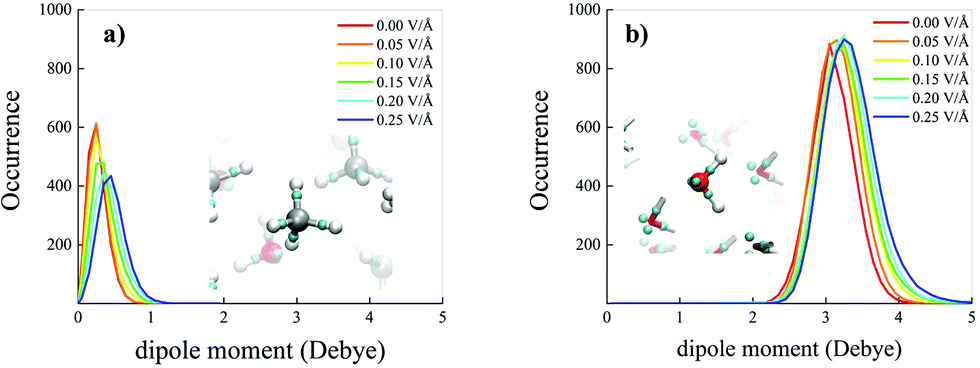 | ||
| Fig. 4 Molecular dipole moment distributions of methane (a) and water (b) in a methane–water liquid mixture under the action of increasing field strengths (see legends). Dipole moments are determined from the Maximally Localised Wannier Functions (MLWFs) centres, whose representation is depicted in the insets (small cyan spheres) both in a methane (a) and in a water (b) molecule. | ||
Such an apparently different behaviour of the field-induced effects on the dipole moment distributions may be partially understood in terms of the different polarisation effects that the potential electrostatic gradient produces on methane and water molecules. A key quantity capable of rationalising the molecular electronic structure in a relationship to the nuclear arrangement is represented by the Maximally Localised Wannier Functions (MLWFs).64,71 The centres of these functions can be interpreted as the quantum counterpart of the classical electron pair concept. This way, oxygen atoms in neat liquid water are typically surrounded by four Wannier centres, two representing the lone pairs, located at a distance of ∼0.3 Å from the oxygen, and two marking the covalent bonds with the hydrogen atoms, located at an average distance of ∼0.5 Å from the oxygen. The separation between the Wannier centres identifying a covalent bond (X) and the closest hydrogen atom (H) gives information tightly related to the stiffness and polarisation of the bond. Equivalent considerations hold for methane molecules as well, of course. This way, the distributions of the XH distances between the Wannier centres of the covalent bonds and their closest hydrogen atoms have been determined as a function of the electric field strength both for methane and water molecules, as shown in Fig. 5a and b, respectively.
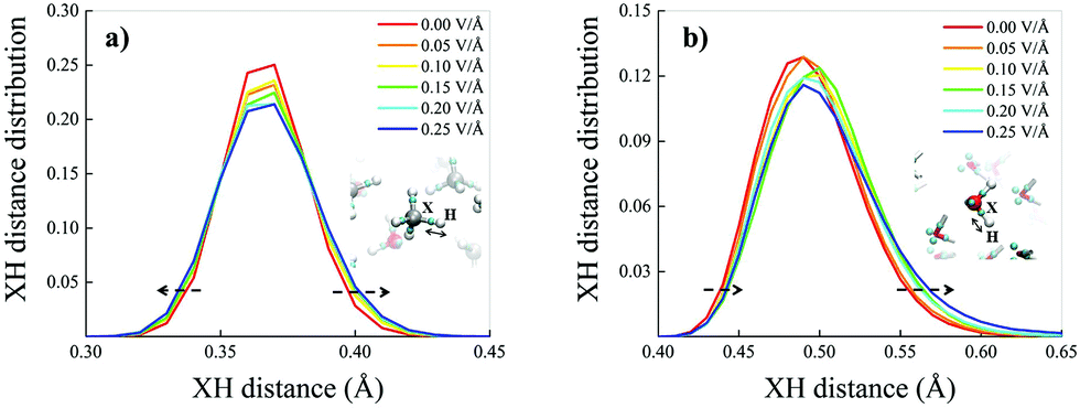 | ||
| Fig. 5 Distributions of the distances between the hydrogen atoms and the first-neighbouring Wannier centres for methane (a) and water (b) molecules in the bulk liquid methane–water mixture for different field strengths (see legends). In the insets, cyan spheres represent Wannier centres whilst white, grey, and red colouring identify hydrogen, carbon, and oxygen atoms, respectively. Dashed arrows are guides for the eyes magnifying some of the field-induced modifications. | ||
Also because of the higher isotropic character of the methane molecules, the median of the XH distance distribution does not move towards larger values of the XH distance but the distribution gets only slightly broader under the action of increasingly stronger fields (Fig. 5a). In contrast, the water XH distance distribution not only gets slightly broader upon increasing the field intensity, but also sizably moves towards larger XH distances, indicating that the OH covalent bonds of the water molecules are significantly weakened by the field, as shown in Fig. 5b. In fact, when an OH covalent bond is stretched during a transient proton transfer event, its Wannier centre shifts towards the oxygen atom.13 This means that whereas the electric field does not alter the structural integrity of the methane molecules, it progressively tends to cleave some of the OH covalent bonds of the water molecules. Finally, the fact that the XH distance distribution of methane changes almost symmetrically under the field action whereas that ascribed to the water molecules is modified in an asymmetrical manner indirectly suggests that fractions of water molecules orient towards the field direction, as also proven in ref. 70 and 72 by similar simulations of aqueous systems. This way, polarisation effects produced by the external field are also enhanced by local contributions stemming from sets of water dipoles concertedly oriented towards the field axis. This combined polarisation effect leads to the cleavage of some of the OH covalent bonds, to the release of protons and, hence, to the onset of the water counterions in the system.
A useful indicator capable of monitoring either ephemeral transient and permanent proton transfer events is the proton sharing coordinate.30,73 This latter is defined, in the case of water, as δ = dOH − dO′H, where dOH is the covalent bond length of a reference molecule, whereas dO′H represents the length of the H-bond(s) that the reference molecule donates, as depicted in the inset of Fig. 6b. When the proton is transiently closer to the acceptor molecule than to the donor oxygen, then δ > 0. Fig. 6a shows the probability distributions of δ for the water molecules in the bulk liquid methane–water mixture as a function of the field strength. Moreover, the behaviour of the distributions for δ → 0 is highlighted by their logarithmic plots in Fig. 6b. As shown by the tails of the distributions, field intensities equal to 0.25 V Å−1 are able to trigger feeble water ionisation events. However, in order to distinguish between statistical fluctuations of thermal nature and genuine ionisation events produced by the field, larger fractions of proton transfer events have to be recorded to identify a net field-induced molecular dissociation threshold.13 Such a circumstance is fulfilled when the system is subjected to a field strength equal to 0.30 V Å−1, as shown in Fig. 6b. As a consequence, the presence of hydrophobic interactions introduced by the presence of methane molecules does not affect the field-induced dissociation threshold of the water molecules. In fact, the same threshold was recorded also for neat bulk liquid water simulated by means of ab initio molecular dynamics (AIMD) techniques.12,13 Thus, starting from a field intensity of 0.30 V Å−1, a mixture originally composed of neutral methane and water molecules hosts also oxonium (H3O)+ and hydroxide (OH)− ions.
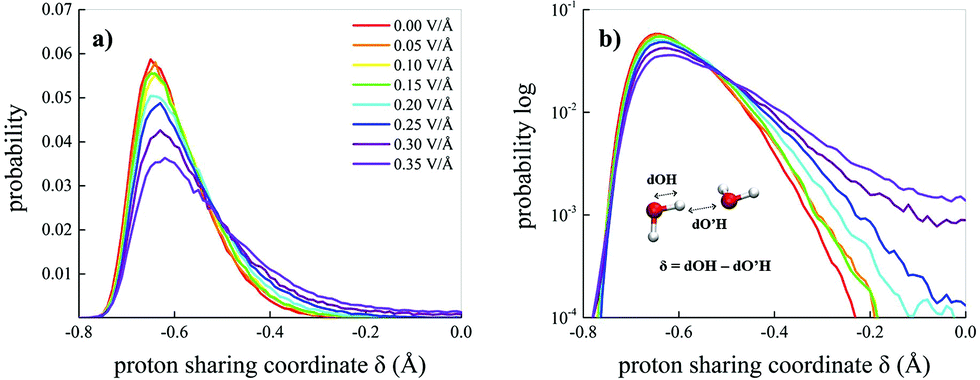 | ||
| Fig. 6 Proton sharing in H-bonds. Probability distributions in the linear (a) and logarithmic (b) scale of the proton sharing coordinate δ of water in the methane–water mixture under the effect of static electric fields at different intensities (see the legend in (a)). In the inset of (b), the definition of the coordinate, which is defined for every hydrogen atom involved in a tight H-bond (i.e., δ ≥ −0.8), is shown. | ||
Differently from what has been observed under extreme pressure regimes, where the pressure-induced formation of the water counterions triggers the dissociation of fractions of methane molecules in methane–water mixtures,3 extreme electric field regimes (i.e., at least up to 0.50 V Å−1) are not capable of doing so. In fact, the motion of the hydrogen atoms belonging to methane molecules and that of the carbon atoms is fully coupled even at those field intensities, as shown in Fig. 7, where the z-component of the mean squared displacement (MSD) of these atoms is displayed at 0.40 V Å−1 (Fig. 7a) and 0.50 V Å−1 (Fig. 7b). Conversely, at these field regimes, hydrogen atoms originally belonging to water molecules are capable of migrating across the H-bond network via the Grotthuss mechanism. In fact, the large mobility acquired under the field action renders the motion of these hydrogen atoms uncoupled from that of the oxygen ones, as shown in Fig. 8. Besides, it is worth mentioning that the MSD curves of the hydrogen atoms shown in Fig. 8 exhibit (quasi)ballistic trends as a function of time because of the externally applied field (i.e., non-random motion of the protons along the field direction). The strong directionality of the correlated proton transfer events triggered and sustained by the field is manifested by the fact that the components of the MSD out of the field direction – such as those parallel to the x and y axes – exhibit trends somehow independent from the intensity of the applied field, as shown in Fig. 9.
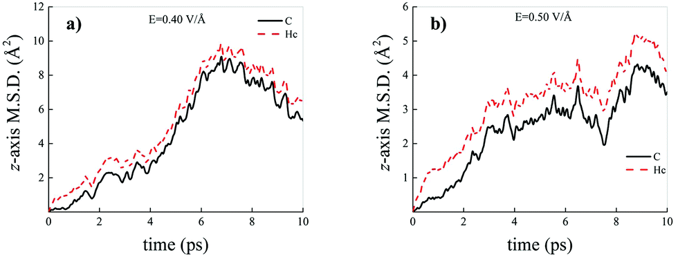 | ||
| Fig. 7 Mean squared displacement (MSD) projected onto the electric field direction (z-axis) of the hydrogen atoms belonging to methane molecules (red dashed curves) and of the carbon atoms (black solid curves) composing the methane–water mixture at field strengths equal to 0.40 V Å−1 (a) and 0.50 V Å−1 (b). | ||
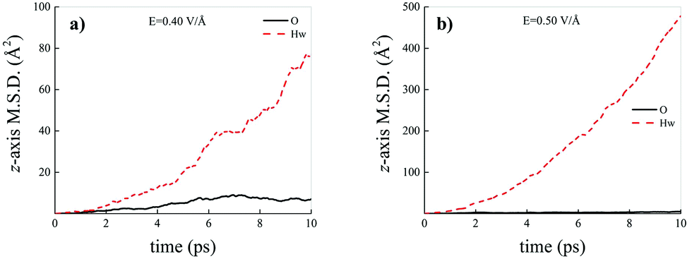 | ||
| Fig. 8 Mean squared displacement (MSD) projected onto the electric field direction (z-axis) of the hydrogen atoms belonging to water molecules (red dashed curves) and of the oxygen atoms (black solid curves) composing the methane–water mixture at field strengths equal to 0.40 V Å−1 (a) and 0.50 V Å−1 (b). | ||
 | ||
| Fig. 9 Cartesian components of the mean squared displacement (MSD) of the hydrogen atoms belonging to water molecules composing the methane–water mixture at field strengths equal to 0.20 V Å−1 (a), 0.30 V Å−1 (b), 0.40 V Å−1 (c), and 0.50 V Å−1 (d). | ||
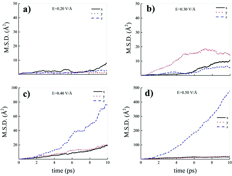
In fact, whereas all MSD components show trends typical of hydrogen atoms covalently bound to their own water molecules for field strengths equal to 0.20 V Å−1 (Fig. 9a) and 0.30 V Å−1 (Fig. 9b), at 0.40 V Å−1 and at 0.50 V Å−1 the MSD Cartesian component parallel to the field direction exhibits a trend magnifying the sizably enhanced mobility of the protons towards the field axis, as displayed in Fig. 9c and d.
This finding clearly indicates that even though the presence of methane molecules certainly interrupts some of the water–water interactions and hence limits the percolation degree of the H-bond network across which protons can migrate, at the investigated molar fraction oxonium cations are still capable of finding traversable pathways parallel to the field axis. In fact, H-bonded “water wires” transmitting protonic defects are frequently observed in the system, as shown in Fig. 10, where the atomistic mechanism of proton migration via a Zundel-to-Zundel Grotthuss mechanism, along with the molecular cooperation between water molecules, is displayed. This way, the protonic current of the system is not significantly affected by the presence of hydrophobic interactions and the proton conductivity is comparable with that recorded in pure water as determined by equivalent AIMD simulations (i.e., σp = 1.3 S cm−1).13
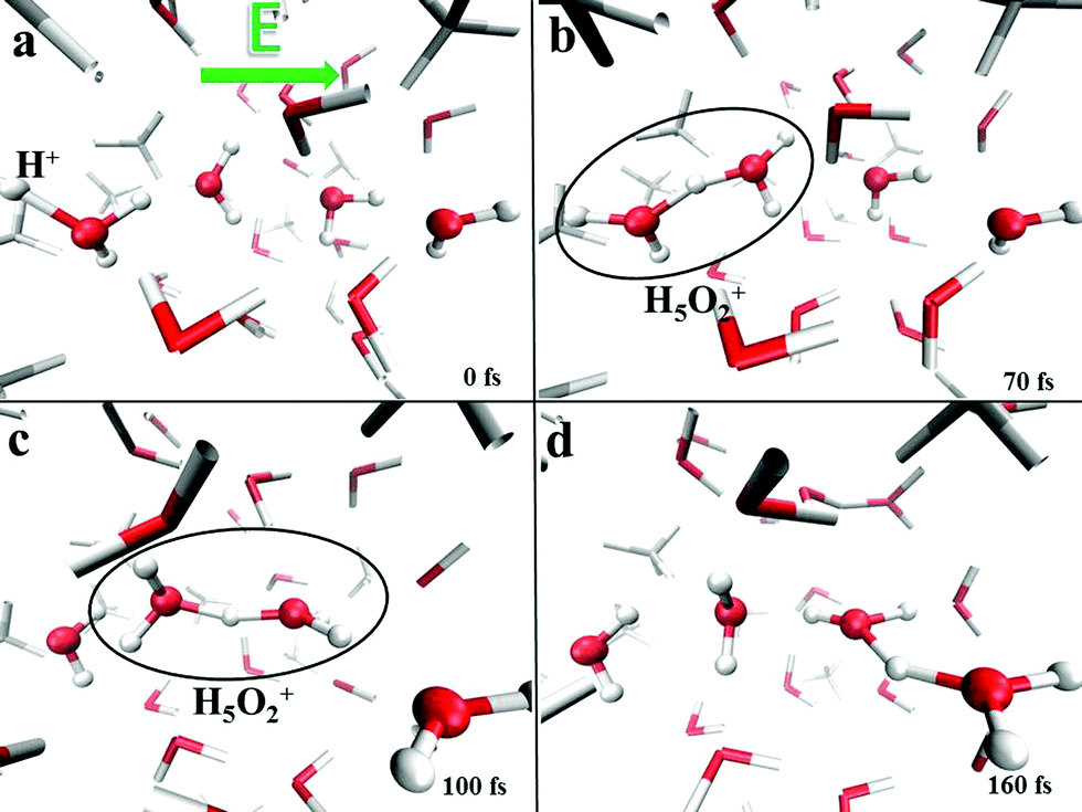 | ||
| Fig. 10 Proton transfer in a liquid methane–water mixture induced by a static and homogeneous electric field. Once a series of H-bonded “water wires” with dipoles heading towards the field direction are formed (a), the formation of a Zundel cation (H5O2)+ can occur (b). If the field strength is intense enough, the Zundel cation suddenly (∼30 fs) propagates (c). Migration of the proton along the field direction via the Grotthuss mechanism partially reverts some of the molecular dipoles (d). | ||
4 Conclusions
In this work, results stemming from a series of ab initio molecular dynamics (AIMD) simulations of a liquid mixture of methane and water at zero and under finite static and homogeneous electric fields have been reported. Although field-induced effects on the intermolecular structure are manifested only by means of a weak structuring of the water subsystem, net modifications produced by the externally applied electrostatic potential gradient are recorded on the electronic structure of the methane–water mixture. In fact, a systematic increment of the magnitude of the molecular dipoles is detected both in methane and in water. Moreover, field-induced polarisation effects have been measured via statistical analysis of the Maximally Localised Wannier Functions (MLWFs) centres behaviour, which revealed that the stiffness of all covalent bonds present in the system – either CH or OH – is altered by field intensities beyond 0.10 V Å−1. However, whereas the isotropic nature of the methane molecules leads to a symmetric modification of the distribution of the distances between the MLWFs centres located on the covalent bonds and the hydrogen atoms belonging to methane molecules, asymmetrical and more pronounced changes of the respective distribution are detected for the water molecules upon field exposure. This finding not only indicates that water dipoles are re-oriented towards the field direction at these low-to-moderate field regimes, but also that the OH covalent bonds are weakened by the applied field to a larger extent with respect to the CH bonds. In fact, the field is capable of disrupting some of the water covalent bonds and, starting from a field intensity of 0.30 V Å−1, a mixture originally composed of neutral methane and water molecules hosts also oxonium (H3O)+ and hydroxide (OH)− ions. However, in contrast to what has been observed in the same mixture upon pressurisation (∼50 GPa), where the presence of the water counterions triggers methane ionisation and complex chemical reactions,3 methane molecules preserve their integrity up to the strongest field explored in the current investigation (i.e., 0.50 V Å−1).Beyond the water dissociation threshold (0.30 V Å−1), the field is capable of sustaining correlated proton transfer events and oxonium ions diffuse across the H-bond network via the Grotthuss mechanism in a Zundel-to-Zundel fashion. Interestingly, neither the field-induced molecular dissociation of neat water (i.e., 0.30 V Å−1)12,13 nor the proton conductivity typical of pure aqueous samples at these field regimes (i.e., 1.3 S cm−1)13 are affected by the presence of the hydrophobic interactions introduced by methane molecules. This finding indicates that even though the presence of methane molecules interrupts some of the water–water spatial correlations and limits the percolation degree of the H-bond network across which protons can migrate, at the investigated methane–water molar fraction (i.e., 0.4:0.6) protons are still capable of finding traversable pathways along H-bonded molecular “water wires” preferably oriented towards the field axis.
Author contributions
Conceptualization: G. C. and F. S.; data curation: G. C.; formal analysis: G. C.; investigation: G. C.; methodology: G. C.; resources: J. S.; validation: G. C., J. S., and F. S.; writing – original draft: G. C.; writing – review & editing: G. C., J. S., and F. S.Conflicts of interest
There are no conflicts to declare.References
- M. Podolak, W. Hubbard and D. Stevenson, Models of Uranus' interior and magnetic field, Nucl. Phys. A, 1991, 29–61 Search PubMed.
- W. J. Nellis, D. C. Hamilton, N. C. Holmes, H. B. Radousky, F. H. Ree, A. C. Mitchell and M. Nicol, Science, 1988, 240, 779–781 CrossRef CAS PubMed.
- M.-S. Lee and S. Scandolo, Nat. Commun., 2011, 2, 185 CrossRef PubMed.
- R. Car and M. Parrinello, Phys. Rev. Lett., 1985, 55, 2471 CrossRef CAS PubMed.
- R. W. Nunes and X. Gonze, Phys. Rev. B: Condens. Matter Mater. Phys., 2001, 63, 155107 CrossRef.
- R. Resta, Phys. Rev. Lett., 1998, 80, 1800 CrossRef CAS.
- X. Gonze, P. Ghosez and R. W. Godby, Phys. Rev. Lett., 1995, 74, 4035 CrossRef CAS PubMed.
- F. Ancilotto, G. L. Chiarotti, S. Scandolo and E. Tosatti, Science, 1997, 275, 1288–1290 CrossRef CAS PubMed.
- E. M. Stuve, Chem. Phys. Lett., 2012, 520, 1–17 CrossRef.
- Z. Hammadi, M. Descoins, E. Salançon and R. Morin, Appl. Phys. Lett., 2012, 101, 243110 CrossRef.
- W. K. Lee, et al. , Nano Res., 2013, 6, 767–774 CrossRef CAS.
- A. M. Saitta, F. Saija and P. V. Giaquinta, Phys. Rev. Lett., 2012, 108, 207801 CrossRef PubMed.
- G. Cassone, J. Phys. Chem. Lett., 2020, 11, 8983–8988 CrossRef CAS PubMed.
- A. C. Aragones, N. L. Haworth, N. Darwish, S. Ciampi, N. J. Bloomfield, G. G. Wallace, I. Diez-Perez and M. L. Coote, Nature, 2016, 531, 88–91 CrossRef CAS PubMed.
- F. Che, J. T. Gray, S. Ha, N. Kruse, S. L. Scott and J.-S. McEwen, ACS Catal., 2018, 8, 5153–5174 CrossRef CAS.
- G. Cassone, F. Pietrucci, F. Saija, F. Guyot and A. M. Saitta, Chem. Sci., 2017, 8, 2329–2336 RSC.
- S. Shaik, D. Mandal and R. Ramanan, Nat. Chem., 2016, 8, 1091–1098 CrossRef CAS PubMed.
- Z. Wang, D. Danovich, R. Ramanan and S. Shaik, J. Am. Chem. Soc., 2018, 140, 13350–13359 CrossRef CAS PubMed.
- G. Cassone, J. Sponer, S. Trusso and F. Saija, Phys. Chem. Chem. Phys., 2019, 21, 21205–21212 RSC.
- P. L. Geissler, C. Dellago, D. Chandler, J. Hutter and M. Parrinello, Science, 2001, 291, 2121–2124 CrossRef CAS PubMed.
- P. G. Bolhuis, D. Chandler, C. Dellago and P. L. Geissler, Ann. Rev. Phys. Chem., 2002, 53, 291–318 CrossRef CAS PubMed.
- M. Chen, L. Zheng, B. Santra, H.-Y. Ko, R. A. DiStasio, M. L. Klein, R. Car and X. Wu, Nat. Chem., 2018, 10, 413–419 CrossRef CAS PubMed.
- V. Rosza, D. Pan, F. Giberti and G. Galli, Proc. Natl. Acad. Sci. U. S. A., 2018, 115, 6952–6957 CrossRef PubMed.
- A. Hassanali, M. K. Prakash, H. Eshet and M. Parrinello, Proc. Natl. Acad. Sci. U. S. A., 2011, 108, 20410–20415 CrossRef CAS PubMed.
- A. Hassanali, F. Giberti, J. Cuny, T. D. Kühne and M. Parrinello, Proc. Natl. Acad. Sci. U. S. A., 2013, 110, 13723–13728 CrossRef CAS PubMed.
- Z. Futera, J. S. Tse and N. J. English, Sci. Adv., 2020, 21, eaaz2915 CrossRef PubMed.
- M. Ceriotti, G. Bussi and M. Parrinello, Phys. Rev. Lett., 2009, 103, 030603 CrossRef PubMed.
- M. Ceriotti, D. E. Manolopoulos and M. Parrinello, J. Chem. Phys., 2011, 134, 084104 CrossRef PubMed.
- M. Ceriotti and D. E. Manolopoulos, Phys. Rev. Lett., 2012, 109, 100604 CrossRef PubMed.
- M. Ceriotti, J. Cuny, M. Parrinello and D. E. Manolopoulos, Proc. Natl. Acad. Sci. U. S. A., 2013, 110, 15591–15596 CrossRef CAS PubMed.
- J. Lan, V. V. Rybkin and M. Iannuzzi, J. Phys. Chem. Lett., 2020, 11, 3724–3730 CrossRef CAS PubMed.
- T. E. Markland and M. Ceriotti, Nature Reviews, 2018, 2, 0109 CrossRef CAS.
- D. Laage, T. Elsaesser and J. T. Hynes, Struct. Dyn., 2017, 4, 044018 CrossRef PubMed.
- A. Kundu, F. Dahms, B. P. Fingerhut, E. T. J. Nibbering, E. Pines and T. Elsaesser, J. Phys. Chem. Lett., 2019, 10, 2287–2294 CrossRef CAS PubMed.
- S. Laporte, F. Finocchi, L. Paulatto, M. Blanchard, E. Balan, F. Guyot and A. M. Saitta, Phys. Chem. Chem. Phys., 2015, 17, 20382–20390 RSC.
- S. Laporte, F. Pietrucci, F. Guyot and A. M. Saitta, J. Phys. Chem. C, 2020, 124, 5125–5131 CrossRef CAS.
- F. Creazzo and S. Luber, Appl. Surf. Sci., 2021, 570, 150993 CrossRef CAS.
- G. Cassone, A. Sofia, G. Rinaldi and J. Sponer, J. Phys. Chem. C, 2019, 123, 9202–9208 CrossRef CAS.
- G. Cassone, A. Sofia, J. Sponer, A. M. Saitta and F. Saija, Molecules, 2020, 25, 3371 CrossRef CAS PubMed.
- G. Cassone, P. V. Giaquinta, F. Saija and A. M. Saitta, J. Chem. Phys., 2015, 142, 054502 CrossRef PubMed.
- N. J. English and J. M. D. MacElroy, J. Chem. Phys., 2004, 120, 10247 CrossRef CAS PubMed.
- C. J. Waldron and N. J. English, J. Chem. Phys., 2017, 147, 24506 CrossRef PubMed.
- C. J. Waldron and N. J. English, J. Chem. Thermod., 2018, 117, 68–80 CrossRef CAS.
- T. Xu, X. Lang, S. Fan, Y. Wang and J. Chen, Comput. Theo. Chem., 2019, 1149, 57–68 CrossRef CAS.
- J. Hutter, M. Iannuzzi, F. Schiffmann and J. VandeVondele, Wiley Interdiscip. Rev.: Comput. Mol. Sci., 2014, 4, 15–25 CAS.
- J. Vandevondele, M. Krack, F. Mohamed, M. Parrinello, T. Chassaing and J. Hutter, Comput. Phys. Commun., 2005, 167, 103–128 CrossRef CAS.
- R. D. King-Smith and D. Vanderbilt, Phys. Rev. B: Condens. Matter Mater. Phys., 1993, 47, 1651–1654 CrossRef CAS PubMed.
- R. Resta, Rev. Mod. Phys., 1994, 66, 899–915 CrossRef CAS.
- M. V. Berry, Proc. R. Soc. London, Ser. A, 1984, 392, 45 Search PubMed.
- P. Umari and A. Pasquarello, Phys. Rev. Lett., 2002, 89, 157602 CrossRef CAS PubMed.
- N. J. English and C. J. Waldron, Phys. Chem. Chem. Phys., 2015, 17, 12407–12440 RSC.
- R. W. Nunes and D. Vanderbilt, Phys. Rev. Lett., 1994, 73, 712 CrossRef CAS PubMed.
- X. Gonze, P. Ghosez and R. W. Godby, Phys. Rev. Lett., 1997, 78, 294 CrossRef CAS.
- M. R. Walsh, C. A. Koh, E. D. Sloan, A. K. Sum and D. T. Wu, Science, 2009, 326(1095), 1095–1098 CrossRef CAS PubMed.
- H. Docherty, A. Galindo, C. Vega and E. Sanz, J. Chem. Phys., 2006, 125, 074510 CrossRef CAS PubMed.
- C. G. Pruteanu, G. J. Ackland, W. C. K. Poon and J. S. Loveday, Sci. Adv., 2017, 3, e1700240 CrossRef PubMed.
- M. Krack, Theor. Chem. Acc., 2005, 114, 145–152 Search PubMed.
- A. D. Becke, Phys. Rev. A: At., Mol., Opt. Phys., 1988, 38, 3098 CrossRef CAS PubMed; C. Lee, W. Yang and R. G. Parr, Phys. Rev. B: Condens. Matter Mater. Phys., 1988, 37, 785 CrossRef PubMed.
- S. Grimme, J. Antony, S. Ehrlich and H. Krieg, J. Chem. Phys., 2010, 132, 154104 CrossRef PubMed.
- S. Grimme, S. Ehrlich and L. Goerigk, J. Comput. Chem., 2011, 32, 1456–1465 CrossRef CAS PubMed.
- I.-C. Lin, A. P. Seitsonen, I. Tavernelli and U. Rothlisberger, J. Chem. Theory Comput., 2012, 8, 3902–3910 CrossRef CAS PubMed.
- A. Bankura, A. Karmakar, V. Carnevale, A. Chandra and M. L. Klein, J. Phys. Chem. C, 2014, 118, 29401–29411 CrossRef CAS.
- M. J. Gillan, D. Alfé and A. Michaelides, J. Chem. Phys., 2016, 144, 130901 CrossRef PubMed.
- N. Marzari and D. Vanderbilt, Phys. Rev. B: Condens. Matter Mater. Phys., 1997, 56, 12847–12865 CrossRef CAS.
- N. Marzari, A. A. Mostofi, J. R. Yates, I. Souza and D. Vanderbilt, Rev. Mod. Phys., 2012, 84, 1419–1475 CrossRef CAS.
- S. Habershon, G. S. Fanourgakis and D. E. Manolopoulos, J. Chem. Phys., 2008, 129, 074501 CrossRef PubMed.
- A. Witt, S. D. Ivanov, M. Shiga, H. Forbert and D. Marx, J. Chem. Phys., 2009, 130, 194510 CrossRef PubMed.
- G. Bussi, D. Donadio and M. Parrinello, J. Chem. Phys., 2007, 126, 014101 CrossRef PubMed.
- G. Cassone, J. Sponer and F. Saija, Top. Catal., 2021 DOI:10.1007/s11244-021-01487-0.
- Z. Futera and N. J. English, J. Chem. Phys., 2017, 147, 031102 CrossRef PubMed.
- E. Schwegler, G. Galli, F. Gygi and R. Q. Hood, Phys. Rev. Lett., 2001, 87, 265501 CrossRef CAS PubMed.
- G. Cassone, F. Creazzo, P. V. Giaquinta, F. Saija and A. M. Saitta, Phys. Chem. Chem. Phys., 2016, 18, 23164–23173 RSC.
- O. Marsalek and T. E. Markland, J. Phys. Chem. Lett., 2017, 8, 1545–1551 CrossRef CAS PubMed.
| This journal is © the Owner Societies 2021 |