Double layer capacitances analysed with impedance spectroscopy and cyclic voltammetry: validity and limits of the constant phase element parameterization

Abstract

Routinely, cyclic voltammetry (CV) or electrochemical impedance spectroscopy (EIS) are used in electrochemistry to probe the current response of a specimen. For the interpretation of the response, constant phase elements (CPEs) are used in the frequency domain based impedance calculus to parameterize the double layer. In this study, the double layer responses to the two measurement techniques are compared by probing a model-type polished gold electrode under potential and amplitude variation. The equivalent circuit that describes the double layer includes a CPE and is parameterized by impedance data, while a computational impedance-based Fourier transform model (source code disclosed) is used to describe the CV response. With CV, the measured and modelled responses show good agreement at amplitudes below 0.2 V and within a certain scan rate window. At larger amplitudes, the ion arrangement in the double layer is actively changed by the measurement, leading to potential dependencies and deviations from the CPE behaviour. These varying contributions to the impedance measurements are not respected in the impedance calculus that relies on a sinusoidal response. The transition from perturbations of the double layer equilibrium to distortions of the ion arrangements is analysed with both measurement methods.

---

Introduction

The concept of the electrochemical double layer describes the ion arrangement at the interface between electrodes and liquid electrolytes.^1–3 A direct technical use of the phenomena of double layer capacitances (DLC) manifests itself in electrochemical capacitors.⁴ Capacitive contributions in the double layer arise from a dielectric polarization of the electrolyte, charge separation by ion displacement and adsorption of ions or molecules¹ and are typically probed with electrochemical impedance spectroscopy (EIS) or cyclic voltammetry (CV).⁵

Potentiostatic EIS is typically used to probe an equilibrated electrode at a constant potential by a small amplitude sinusoidal perturbation. The impedance calculus operates in the frequency domain, where the response to the perturbation is described by a sinusoidal answer with a phase and an amplitude.^6,7 Double layer capacitances are typically parameterized by constant phase elements (CPEs),^8–11 which are defined by frequency independent phase angles.^12,13 The CPE behaviour with its frequency independent ratio or resistive to capacitive contributions is for instance found in transmission lines,^12,14,15 which may be from a physicochemical perspective responsible for the CPE behaviour of double layers in EIS.¹⁶

CV is another standard method in electrochemistry, in which the response of an electrode is probed in the time domain under a triangular potential variation.¹⁷ This method is typically used to examine electrochemical redox behaviour^18–20 or to probe capacitances.^4,5,21 The response in the time domain to the triangular potential variation is typically non-linear. For example, when a capacitor is examined with CV the response is of a rectangular form, which means that the harmonic content of the perturbation is different from that of the response.²² Thus, the potential-current profile measured by CV can contain potential dependencies and non-linear contributions that are typically not evaluated with the reduced information in the impedance calculus.

Describing non-sinusoidal waveforms by Fourier transformation and analysing an equivalent circuit's response with a following inverse Fourier transformation is a standard method in electrical engineering and was recently reported for the case of CV with a CPE.²³ Thus, the frequency domain based impedance calculus can be used to model the response in the time domain. A similar approach is presented in the current study (detailed differences in the ‘model section’) with the focus to analyse validity and limits of the CPE based description of the double layer and the underlying potential dependence of its response.

To analyse the double layer response in detail, a polished gold electrode is probed with EIS and CV under amplitude variation. On the basis of the modelled and measured results, the outcomes of both measurement techniques are directly compared. This study shows that the examined dynamics of the double layer crucially depends on the applied amplitude. Small amplitudes can be interpreted as a perturbation of the double layer equilibrium whereas large amplitudes lead to a distortion of the equilibrium by a pervasive rearrangement of the ion arrangement in the double layer. With a combined experimental and modelled study of the response, the transition from perturbations to distortions with changing amplitude is shown. Both measurement methods are discussed to complement one another, impedance with its easy calculus to parameterize the response at small amplitudes and CV to analyse the dynamic potential dependence and double layer distortion at large amplitudes.

Experimental

A three electrode electrochemical setup was used for measurements in this study. An illustration of the in-house made setup is provided in the ESI† to this article. In brief, a polished gold (Junker Edelmetalle GmbH, purity 99.99%) plate was used as the working electrode. The gold plate was polished with 1 μm diamond solution (Struers). To remove organic or metallic impurities on the surface, the gold plate was rinsed with acetone and water, immersed in a solution of 5 M H₂SO₄ and 10% H₂O₂ and thoroughly rinsed with water again. Sealed with a Viton flat sealing (Reichelt Chemietechnik GmbH), an electrochemically active surface area of 0.78 cm² was exposed to a 0.1 M perchloric electrolyte (Alfa Aesar). An Ag/AgCl reference electrode (Metrohm) was used in combination with a Luggin capillary, which was approximately 4 mm far away from the working electrode. The compartment of the counter electrode (a gold wire coil) has been connected with a capillary of 5 mm diameter to the main compartment with the sample. Argon was purged with a rate of 50 mL min⁻¹ through a round shaped polytetrafluoroethylene frit (Bola) with a distance of 10 mm to the gold plate. Thus, oxygen impurities are reduced in order to minimize their electrocatalytic reduction on the gold sample.

The three electrode cell was operated with a Metrohm Modular line potentiostat. The electrolyte has a pH value of 1 and in combination with the Ag/AgCl reference (0.197 V vs. RHE) a combined offset of 0.256 V vs. RHE which was added to the measurements, so that all the potentials stated in this study refer to that of the RHE. The first and second cycle of the CV measurements often deviate from those that follow, for which all experimental CV data shown in this study refer to the fourth of five measured cycles. Scan rates and potential ranges of the CV measurements were varied, in order to discuss parameter dependencies and the limits for the applicability of the developed model.

Theory and computational method

In this study, the response of the double layer of the polished gold electrode to CV and EIS is parameterized by a constant phase element (CPE), while the electrolytic ion conduction of the bulk electrolyte is described by the resistance R_s. Redox-reactions are not included in the model considerations, as these typically only play a minor role in the case of the chemically inert gold electrode considered. Several equivalent circuits for the double layer of gold in perchloric acid were compared in a recent study,¹⁶ in which the used equivalent circuit shows a good representation of the measured impedance spectra. The CPE takes into account the potential-driven ion movement and the related shielding/adsorption of the ions at the electrode surface, whereas the resistance accounts for the electrolyte resistance. This equivalent circuit is the most direct representation of the experimental data presented, whereas any equivalent circuit that fits to the impedance spectra is feasible to model the CV response with the here presented method.

The impedance Z_CPE of a constant phase element is characterized by

where i denotes the complex number, ω the angular frequency, ξ the proportionality factor and n the exponent of the CPE. The impedance of the equivalent circuit in Fig. 1 equals:

Z_EQC = R_s + Z_CPE (2)

The derivation of the real and imaginary part of the impedance is derived elsewhere in detail.¹⁶

Fig. 1 Equivalent circuit used in this study, with the electrolyte resistance R_s and the constant phase element Z_CPE.

Fig. 2 provides a schematic sketch of the method used to calculate the response of the equivalent circuit in cyclic voltammetry. This method consists of four steps, which are linked to the schematic sketch: (A) the triangular potential variation is approximated by its Fourier series²⁴ (harmonically related sinusoidal functions with weighted amplitudes). (B) The response of each term of the Fourier series is calculated by the impedance calculus in the frequency domain. (C) Based on phase angle and impedance value, the individual sinusoidal current responses are calculated in the time domain. By superposition of the individual current responses, the current is obtained as a function of time. (D) The typical plot of I(E) that is used to graph cyclic voltammetry data is derived by substitution of the time in in response function I(t) by E(t).

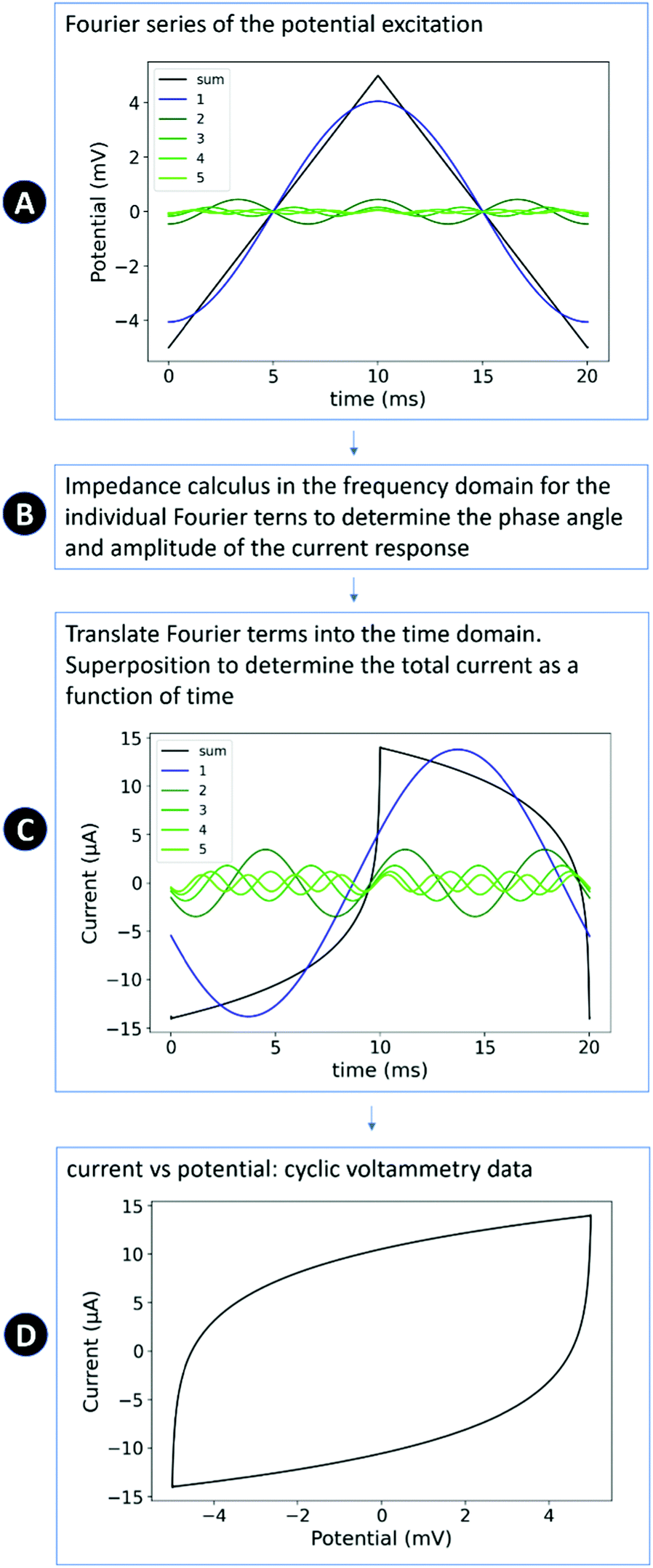Fig. 2 Sketch of the method used to calculate the CV response of CPEs. Black lines: full potential variation or current response calculated with a Fourier series of 500 terms. Blue line: base frequency. Green lines: the first four higher harmonics of the Fourier representation. An explanation of the individual steps is given in the text.

A recent study of Yun and Hwang reported a similar approach to compare impedance and cyclic voltammetry data,²³ using an inverse Fourier transformation instead of the numerical superposition of the individual currents in the time domain. From theory both approaches are expected to lead to the same result. Unfortunately, the source codes of Yun and Hwang were not reported so it is not possible directly to compare their approach to the one presented here. In the following, the physical–mathematical background of the developed model approach is described in detail.

The triangular potential variation E(t) during cyclic voltammetry can be approximated by its Fourier series in the form of

where A denotes the amplitude, ω₀ the angular frequency of the periodic potential variation and t the time. From the latter equation the amplitude A^E_k of the individual terms of the sum can be extracted:The triangular term of the individual contributions in the series can be related to the potential variation frequency ω₀ by

cos((2k − 1)ω₀t) = sin(ω_kt − ϕ^E_k), (5)

with ω_k = (2k − 1)ω₀ and ϕ^E_k = −3π/2. Thus, each individual wave can be described by a sinusoidal core wave with an individual amplitude, frequency and phase angle. The current response with the amplitude A^I_k and phase angle ϕ^I_k of the CPE is of the form:

I_k(t) = A^I_ksin(ω_kt − ϕ^I_k) (6)

The amplitude of the current equals the amplitude of the input wave divided by the value of the impedance:Adding the phase angle of the potential variation from the Fourier series to that obtained from the impedance calculus, the phase angle of the current can be determined to:Based on the latter three equations the individual current response is calculated by:Adding the individual currents in the time domain leads to the overall current I(t):

I(t) = ∑I_k (10)

The Fourier series is special case of the more general Fourier transformation, which can be used to translate a function in the time domain to the frequency domain and vice versa. A Fourier transformation of I(t) is mathematically equal to the superposition of the Fourier transformed individual terms I_k, which justifies the presented approach that relies on the calculation of the individual sinusoidal waves with the impedance calculus in the frequency domain.

The procedure to calculate the CV response was implemented in the form of a computational code in the programming language Python. The source code is supplied in the ESI† to this article. The Fourier series of the potential variation is represented by 500 terms in this study, which provides a good resolution of the unsteady parts of the triangular function at its inversion points. These 500 terms span with reference to eqn (3) over three decades in the frequency. The offset of experimentally applied potentials plus half of the potential variation amplitude was added to the modelled response, in order to resemble the applied potential during the experiments.

Results and discussion

In the following, the responses of a polished gold electrode in 0.1 M perchloric acid to electrochemical impedance spectroscopy (EIS) and cyclic voltammetry (CV) measurements are analysed. The impedance parameterization of the equivalent circuit is considered under amplitude and potential amplitude variation. Based on this parameterization, the CV response is calculated and compared to the measured results. All amplitudes stated refer to peak-to-peak values.

Impedance data

The double layer capacitance obeys an intrinsic potential dependence that is for example used to determine the potential of zero charge.^25–29 At small amplitudes, impedance spectroscopy probes a perturbation of the double layer equilibrium. The capacitance dispersion an import measure for capacitive contributions of the double layer to the impedance spectrum and it was previously reported¹⁶ as:The capacitance dispersion can show small changes in the response that are often not visible in a standard impedance plot, for which this is graphed with the impedance data.

Fig. 3A shows the impedance spectra with the value of the impedance, the phase angle and the capacitance dispersion (eqn (11)). The potential was varied stepwise after a spectrum was recorded, while an amplitude of 20 mV was used. The measured capacitance dispersions were fitted with a previously reported procedure¹⁶ (least-squares method) to parameterize the equivalent circuit. The same reference supplies a detailed discussion of the impedance spectra of gold in perchloric acid. In brief, the spectra can be interpreted as follows: above 8 kHz measurement errors dominate the capacitance dispersion. Below 1 Hz the phase angle increases due to the reduction of oxygen impurities. In between these frequencies the response is dominated by the double layer parameterization and its relaxation. The electrolyte resistance was determined at 50 kHz from the real part of the impedance to R_s = 13.5 Ω.

Fig. 3 Electrochemical impedance data of the polished gold electrode in 0.1 perchloric acid. (A) Impedance spectra with a peak-to-peak amplitude of 0.02 V at four different potentials (0.1, 0.4, 07 and 1 V), showing the value of the impedance |Z|, its phase angle the capacitance dispersion. Scatter: measured impedance. Solid lines: fitted impedance spectra of the equivalent circuit graphed in Fig. 2. (B) Amplitude variation from 0.05 to 0.8 V peak-to-peak around a mean potential of 0.6 V. (C) Potential dependence of the parameters n and ξ of the CPE. (D) Effect of amplitude on the parameters of the CPE.

Fig. 3C shows the CPE parameters determined from individual impedance spectra that were partly shown in Fig. 3A, displaying that the parameterization of the double layer by the CPE depends on the potential. The parameter ξ reflects an inverse relation to the capacitive contributions to the impedance, for which a larger capacitance in Fig. 3A means a lower value of ξ in Fig. 3C.

Fig. 3B shows the impedance spectra of the polished gold electrode under amplitude variation. From an amplitude of 0.02 V to 0.2 V the impedance spectra and the capacitance dispersion do not significantly change. With larger amplitudes the capacitive contributions to the impedance increases below 100 Hz. In addition, with these amplitudes the spectra show additional features between 0.5 and 5 kHz and a deviation of the phase angle from the constant phase behaviour below 10 Hz, which are not described by the fits of the equivalent circuit. Even if more components are added to the equivalent circuit in order to fit to the data, the mechanisms of the potential dependence cannot be described by a potential independent and static equivalent circuit. Due to the potential dependence higher harmonics have to be taken into account, which however cannot be analysed with most modern impedance analysers.

Fig. 3D shows the constant phase element parameters as a function of the amplitude variation around a mean potential of 0.6 V that were derived from the impedance spectra in Fig. 3B. Below an amplitude of 0.2 V, the constant phase elements parameters just slightly change. As the capacitance dispersion in Fig. 3B shows a significant increase of the capacitance at amplitudes above 0.2 V, the parameters start to change. The value of ξ decreases, resembling a higher capacitive contribution to the response.

CV data

In CV the potential variation and the response are both of high harmonic content and can be described by a series of discrete frequencies and amplitudes in terms of a Fourier series. The triangular potential variation is typically characterized by the scan rate ν and the potential range ΔE. From both parameters the base frequency f_CV (i.e. the first-term frequency of the Fourier series) of the triangular function for the CV measurement can be calculated as:The factor of two in the denominator considers the up- and down-going branch that resemble a full potential scan. The amplitude E₀ in the frequency domain and potential range ΔE in the time domain are a Fourier-pair of identical meaning, for which both terms can be equally used. Fig. 4 displays the relation of scan rate, amplitude and frequencies for a systematic parameter variation in an interval between 0.05–1.0 V for the amplitude.

Fig. 4 Relation of scan rate to frequency as a function of the amplitude in CV on the basis of eqn (12). The greenish shaded region corresponds to the frequency region of constant phase behaviour of the data graphed in Fig. 3A.

The frequency window between 1 Hz and 100 Hz in which the responses to amplitudes below 0.2 V are of a constant phase character (compare to Fig. 3B) are shaded greenish in Fig. 4. With a scan rate of 0.1 V s⁻¹ an amplitude smaller as 0.05 V has to be chosen in order to reach a frequency higher as 1 Hz and to remain in the greenish area of the plot. With a scan rate of 1 V s⁻¹, amplitudes below 0.5 V lead to frequencies above 1 Hz. With CV it is not possible to exceed a frequency of 100 Hz, as scan rates above 1 V s⁻¹ or amplitudes below 10 mV are typically not reasonable choices to obtain decent CV data. Accordingly, frequencies higher than the frequency window of constant behaviour are not reachable with CV.

The lowest frequency of the Fourier series is the base frequency, while the highest frequency is with the 500 terms used in the Fourier series three decades higher than the base frequency. The equivalent circuit reasonably described the impedance data above 1 Hz, for which the CV model is expected to also describe the data for base frequencies of 1 Hz or higher. However, at lower frequencies, the charge transfer of oxygen impurities is not included, for which deviations have to be expected. The double layer resembles a CPE in just a certain frequency window. The higher harmonic perturbations (as described by the Fourier series) by cyclic voltammetry however span with the used 500 terms of the frequency over three decades in frequency. Accordingly, the CV-response at one frequency contains with its non-linearities the information of an impedance spectrum from the base frequency upwards.

Fig. 5A shows cyclic voltammograms for scan rate variation and a fixed amplitude of 0.05 V and scan rates from 0.01 to 1 V s⁻¹. The current increases towards higher scan rates and the orders of magnitude different currents make the shape of the CVs difficult to compare. In this depiction, the responses for scan rates between 0.1 and 1 V s⁻¹ can be clearly seen and show good agreement of modelled and measured data. The currents at slower scan rates are too small to be compared in this depiction.

Fig. 5 Scan rate variation of modelled (dotted black lines) and experimental (solid coloured lines) CV responses on the polished gold sample with an amplitude of 0.05 V. From the slow to fast scan rates, the corresponding frequencies are 0.1, 0.2, 0.5, 1, 2, 5 and 10 Hz. (A) Current as a function of the potential. (B) Capacitance (current divided by scan rate) as a function of the potential.

To simplify a comparison of the CV data of different scan rates, the currents can be normalized to the scan rates, which results in the dimension of a capacitance (units Farad). Fig. 5B shows the data from Fig. 5A with such a normalization in which the current can be interpreted as capacitive charge/discharge. As a result, the magnitudes of the responses become comparable. Above 0.1 V s⁻¹ measurement and model data agree. Below 0.02 V s⁻¹ and the applied amplitude of 0.05 V, the frequency gets lower than 1 Hz (see Fig. 4). In this frequency range the parameterization by the equivalent circuit is no longer valid (with respect to the impedance data in Fig. 3A), for which increasing deviations between modelled and measured data appear.

Fig. 6 shows the measured and modelled CV response under amplitude variation from 0.05 to 0.8 V and a fixed scan rate of 0.1 V s⁻¹. The CVs were modelled for two cases: (A) with one set of CPE parameters that was obtained from the impedance spectra at 0.05 V and an equilibrium potential of 0.6 V. (B) With individual sets of CPE parameters that were obtained from the impedance measurement with the same amplitude, respectively. At an amplitude of 0.05 V and 0.1 V, the measured and modelled CV show very good agreement. With an amplitude of 0.2 V small deviations start to appear between the measured and the modelled response, whereas at an amplitude of 0.4 V significant differences arise. Towards larger amplitudes, the CVs modelled with the CPE parameters of the 0.05 V amplitude tend to smaller enclosed areas as the modelled data. In contrast, the CPE parameters obtained from the same CV and impedance amplitudes lead to higher enclosed areas.

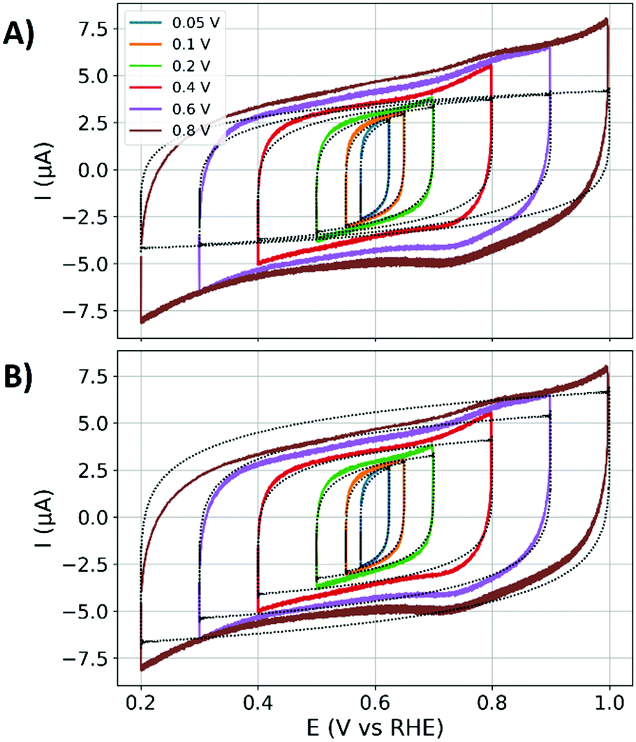Fig. 6 Measured (coloured solid lines) and modelled (dashed black lines) CV responses under amplitude variation from 0.05 to 0.8 V. (A) Equivalent circuit parameterized with the impedance spectrum at an amplitude of 0.05 V. (B) Equivalent circuits parameters for the CV data are taken from the impedance fit with the same amplitude.

Perturbations and distortions of the double layer

The data in Fig. 3A showed the potential dependence of the CPE parameters that was obtained with a stepwise variation of the electrode potential. At amplitude above 0.2 V, these potential dependencies of the double layer also appear in the CV data. The electrode potential affects the static arrangement of the ions in the double layer, including shielding effects and the electronic interaction of the electrode's electronic structure and the double layer.³⁰ The potential dependent changing parameterization of the double layer is not included in the equivalent circuit that is used for the CV response model.

Besides the potential dependence of the double layer, Fig. 3B also showed an amplitude dependence of the response. This amplitude dependence represents the transition from perturbations of the double layer equilibrium to a distortion, in which the applied potential variation actively changes the state of the double layer. Fig. 7 aims to illustrate the differences between a perturbation of the double layer ion arrangement at small amplitudes and a distortion at large amplitudes. In the case of the perturbation, the ions are slightly displaced around their equilibrium positions. At large amplitudes, the ion arrangement is drastically changed, so that the amount of the ions in the inner and outer Helmholtz plane³¹ significantly change. As the boundary condition of the electrode–electrolyte interface is a barrier for the ion migration, the changes in the double layer become more and more asymmetrical, which displays a source for the non-sinusoidal impedance response that may also lead to hysteresis effects.³²

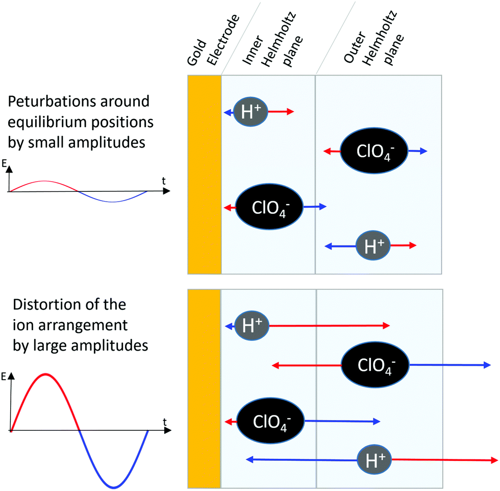Fig. 7 Schematic illustration of perturbations and distortions of the double layer under sinusoidal potential variation and the related movement of protons and perchlorate ions.

Accordingly, small amplitude perturbations of the equilibrium states probe different physicochemical mechanisms than large amplitude distortions of the equilibrium and the related changes of the probe itself. Thus, the influence of the mean potential and amplitude both influence the responses of double layers in CV and EIS.

The impedance data evaluation is meaningful in small potential windows where the one set of parameters describes the response. When the measured and modelled CV data agree in the same potential window, the impedance derived equivalent circuit adequately represents the electrode. However, when the CV data shows additional potential dependent features, the impedance response with the same amplitude will contain non-sinusoidal contributions. In this case the parameterization of the equivalent circuit does not include all appearing potential dependent physicochemical effects of the response. In this case, higher harmonics contribute to the impedance spectra, which however cannot be analysed with most impedance analysers.

To summarize, EIS allows to precisely and easily characterize perturbations of the equilibrium state of the double layer at small amplitudes with the impedance calculus. However, at larger amplitudes the potential dependent contributions are difficult to analyse. In contrast, in CV the response of double layers requires more complex impedance based models, for which it is challenging to parameterize the electrode with the CV data. Yet, the CV data contains all the potential dependent information of the double layer. Accordingly, the choice of the measurement method affects the information content of the probed specimen.³³ The combination of both measurement methods displays a powerful electrochemical toolset to understand the dynamics of the double layer and the transition from perturbations of equilibrium states to distortions of the probed system.

Conclusion

In summary, the response of the double layer of a polished gold electrode has been probed with electrochemical impedance spectroscopy (EIS) and cyclic voltammetry (CV). A constant phase element (CPE) was used to parameterize the response of the double layer. By a Fourier transformation, the impedance calculus in the frequency domain was used to describe the CV response in the time domain. Up to an amplitude of 0.2 V, the experimentally measured impedance is adequately represented by a CPE based parameterization. The CV response modelled with these parameters agrees with the measured data. In this regime, a perturbation of the double layer equilibrium is probed, where the applied potential only slightly impacts the ion arrangement in the double layer. Higher amplitudes lead to significant deviations of the modelled from the measured CV response, while new features appear in the impedance spectra. The static CPE parameterization does not include the potential dependence of the double layer and the related non-sinusoidal contributions to the impedance response, which display a loss of information in the amplitude and phase angle based impedance calculus. These higher amplitudes are associated with a drastic distortion of the ion arrangement double layer, which increase the capacitance and asymmetric ion movements. Impedance is found to be suitable for probing perturbations of equilibrium states at small amplitudes and to parameterize the equivalent circuit, whereas CV enables a detailed analysis of dynamic distortions of the double layer at larger amplitudes where the limits of the validity of the CPE parameterization are exceeded. The presented impedance-based response modelling of double layers in CV and the provided source codes enable to precisely understand the transition from the perturbation to a distortion of a double layer equilibrium as a function of excitation amplitude.

Conflicts of interest

There are no conflicts to declare.

Acknowledgements

This work was supported by the German Federal Ministry of Education and Research (BMBF) within the Project iNew (03SF0589A).

References

1. W. Schmickler and D. Henderson, New models for the structure of the electrochemical interface, Prog. Surf. Sci., 1986, 22, 323–419.
2. A. Groß and S. Sakong, Modelling the electric double layer at electrode/electrolyte interfaces, Curr. Opin. Electrochem., 2019, 14, 1–6.
3. J. Huang and Y. Chen, Combining theory and experiment in advancing fundamental electrocatalysis, Curr. Opin. Electrochem., 2019, 14, A4–A9.
4. Y. Wang, Y. Song and Y. Xia, Electrochemical capacitors: Mechanism, materials, systems, characterization and applications, Chem. Soc. Rev., 2016, 45, 5925–5950.
5. C. C. L. McCrory, S. Jung, J. C. Peters and T. F. Jaramillo, Benchmarking Heterogeneous Electrocatalysts for the Oxygen Evolution Reaction, J. Am. Chem. Soc., 2013, 135, 16977–16987.
6. B.-Y. Chang and S.-M. Park, Electrochemical Impedance Spectroscopy, Annu. Rev. Anal. Chem., 2010, 3, 207–229.
7. M. Popovic, B. Grgur and M. Vojnovic, On the kinetics of the hydrogen evolution reaction on nickel in alkaline solution Part I. The mechanism, J. Electroanal. Chem., 2001, 512, 16–26.
8. P. Córdoba-Torres, T. J. Mesquita, O. Devos, B. Tribollet, V. Roche and R. P. Nogueira, On the intrinsic coupling between constant-phase element parameters α and Q in electrochemical impedance spectroscopy, Electrochim. Acta, 2012, 72, 172–178.
9. B. Piela and P. Wrona, Capacitance of the gold electrode in 0.5 M H₂SO₄ solution: a.c. impedance studies, J. Electroanal. Chem., 1995, 388, 69–79.
10. T. Pajkossy and D. M. Kolb, Double layer capacitance of the platinum group metals in the double layer region, Electrochem. Commun., 2007, 9, 1171–1174.
11. T. Pajkossy, Capacitance dispersion on solid electrodes: anion adsorption studies on gold single crystal electrodes, Solid State Ionics, 1997, 94, 123–129.
12. J. C. Wang, Realizations of Generalized Warburg Impedance with RC Ladder Networks and Transmission Lines, J. Electrochem. Soc., 1987, 134, 1915–1920.
13. D. D. MacDonald, Reflections on the history of electrochemical impedance spectroscopy, Electrochim. Acta, 2006, 51, 1376–1388.
14. J.-B. Jorcin, M. E. Orazem, N. Pébère and B. Tribollet, CPE analysis by local electrochemical impedance spectroscopy, Electrochim. Acta, 2006, 51, 1473–1479.
15. B. Hirschorn, M. E. Orazem, B. Tribollet, V. Vivier, I. Frateur and M. Musiani, Constant-Phase-Element Behavior Caused by Resistivity Distributions in Films: I. Theory, J. Electrochem. Soc., 2010, 157, C452–C457.
16. M. Schalenbach, Y. E. Durmus, S. Robinson, H. Tempel, H. Kungl and R. Eichel, The Physicochemical Mechanisms of the Double Layer Capacitance Dispersion and Dynamics: An Impedance Analysis, Phys. Chem. C, 2021, 125, 5870–5879.
17. J. Heinze, Cyclic Voltammetry-“Electrochemical Spectroscopy”, Angew. Chem., Int. Ed. Engl., 1985, 23, 813–918.
18. M. Schalenbach, F. D. Speck, M. Ledendecker, O. Kasian, D. Goehl, A. M. Mingers, B. Breitbach, H. Springer, S. Cherevko and K. J. J. Mayrhofer, Nickel-Molybdenum alloy catalysts for the hydrogen evolution reaction: Activity and stability revised, Electrochim. Acta, 2017, 259, 1154–1161.
19. S. Ardizzone, G. Fregonara and S. Trasatti, ‘Inner’ And ‘Outer’ Active Surface Electrodes Of RuO₂ Electrodes, Electrochim. Acta, 1989, 35, 263–267.
20. M. Schalenbach, O. Kasian, M. Ledendecker, S. Cherevko, A. Mingers, F. Speck and K. J. J. Mayrhofer, The electrochemical dissolution of noble metals in alkaline media, Electrocatalysis, 2018, 9, 153–161.
21. T. Brousse, D. Belanger and J. W. Long, To Be or Not To Be Pseudocapacitive?, J. Electrochem. Soc., 2015, 162, A5185–A5189.
22. A. Allagui, T. J. Freeborn, A. S. Elwakil and B. J. Maundy, Reevaluation of Performance of Electric Double-layer Capacitors from Constant-current Charge/Discharge and Cyclic Voltammetry, Sci. Rep., 2016, 6, 1–8.
23. C. Yun and S. Hwang, Analysis of the Charging Current in Cyclic Voltammetry and Supercapacitor's Galvanostatic Charging Profile Based on a Constant-Phase Element, ACS Omega, 2021, 6, 367–373.
24. G. P. Tolstov, Fourier Series, Courier Corporation, 2012.
25. J. O. M. Bockris and S. D. Argade, Work Function of Metals and the Potential at Which They Have Zero Charge in Contact with Solutions, J. Chem. Phys., 1968, 49, 5133–5134.
26. S. Trasatti and E. Lust, Modern Aspects of Electrochemistry, 2002, vol. 33.
27. F. Silva, M. J. Sottomayor and A. Hamelin, The temperature coefficient of the potential of zero charge of the gold single-crystal electrode/aqueous solution interface. Possible relevance to gold-water interactions, J. Electroanal. Chem., 1990, 294, 239–251.
28. H. R. Zebardast, S. Rogak and E. Asselin, Potential of zero charge of glassy carbon at elevated temperatures, J. Electroanal. Chem., 2014, 724, 36–42.
29. M. T. Alam, M. Mominul Islam, T. Okajima and T. Ohsaka, Measurements of differential capacitance in room temperature ionic liquid at mercury, glassy carbon and gold electrode interfaces, Electrochem. Commun., 2007, 9, 2370–2374.
30. W. Schmickler, A jellium-dipole model for the double layer, J. Electroanal. Chem., 1983, 150, 19–24.
31. I. V. Zenyuk and S. Litster, Spatially resolved modeling of electric double layers and surface chemistry for the hydrogen oxidation reaction in water-filled platinum-carbon electrodes, J. Phys. Chem. C, 2012, 116, 9862–9875.
32. A. J. Lucio and S. K. Shaw, Effects and controls of capacitive hysteresis in ionic liquid electrochemical measurements, Analyst, 2018, 143, 4887–4900.
33. L. J. Small and D. R. Wheeler, Influence of Analysis Method on the Experimentally Observed Capacitance at the Gold-Ionic Liquid Interface, J. Electrochem. Soc., 2014, 161, H260–H263.

---

Footnote

† Electronic supplementary information (ESI) available: Schematic sketch of the electrochemical cell. Reproduction measurements and discussion of measurement errors. Full range cyclic voltammetry data. Impedance data in Nyquist plot. Chi-squared analysis of the impedance fits. Computer codes for the CV simulation in Python. See DOI: 10.1039/d1cp03381f

---