
cis → trans photoisomerisation of azobenzene: a fresh theoretical look†
Isabella C. D.
Merritt
 ,
Denis
Jacquemin
and
Morgane
Vacher
*
,
Denis
Jacquemin
and
Morgane
Vacher
*
Laboratoire CEISAM – UMR 6230 – CNRS – Université de Nantes, Nantes, France. E-mail: morgane.vacher@univ-nantes.fr; Tel: +33-2-76-64-51-47
First published on 1st July 2021
Abstract
The cis → trans photo-isomerisation mechanism of azobenzene, after excitation to the nπ* and ππ* states, is revisited using high-level ab initio surface hopping mixed quantum-classical dynamics in combination with multi-reference CASSCF electronic structure calculations. A reduction of photoisomerisation quantum yield of 0.10 on exciting to the higher energy ππ* state compared to the lower energy nπ* state is obtained, in close agreement with the most recent experimental values [Ladányi et al., Photochem. Photobiol. Sci., 2017, 16, 1757–1761] which re-examined previous literature values which showed larger changes in quantum yield. By direct comparison of both excitations, we have found that the explanation for the decrease in quantum yield is not the same as for the reduction observed in the trans → cis photoisomerisation. In contrast to the trans → cis scenario, S1 → S0 decay does not occur at ‘earlier’ C–N![[double bond, length as m-dash]](https://www.rsc.org/images/entities/char_e001.gif) N–C angles along the central torsional coordinate after ππ* excitation, as in the cis → trans case the rotation about this coordinate occurs too rapidly. The wavelength dependency of the quantum yield is instead found to be due to a potential well on the S2 surface, from which either cis or trans-azobenzene can be formed. While this well is accessible after both excitations, it is more easily accessed after ππ* excitation – an additional 15–17% of photochromes, which under nπ* excitation would have exclusively formed the trans isomer, are trapped in this well after ππ* excitation. The probability of forming the cis isomer when leaving this well is also higher after ππ* excitation, increasing from 9% to 35%. The combination of these two factors results in the reduction of 0.10 of the quantum yield of photoisomerisation on ππ* excitation of cis-azobenzene, compared to nπ* excitation.
N–C angles along the central torsional coordinate after ππ* excitation, as in the cis → trans case the rotation about this coordinate occurs too rapidly. The wavelength dependency of the quantum yield is instead found to be due to a potential well on the S2 surface, from which either cis or trans-azobenzene can be formed. While this well is accessible after both excitations, it is more easily accessed after ππ* excitation – an additional 15–17% of photochromes, which under nπ* excitation would have exclusively formed the trans isomer, are trapped in this well after ππ* excitation. The probability of forming the cis isomer when leaving this well is also higher after ππ* excitation, increasing from 9% to 35%. The combination of these two factors results in the reduction of 0.10 of the quantum yield of photoisomerisation on ππ* excitation of cis-azobenzene, compared to nπ* excitation.
 Morgane Vacher | Morgane Vacher is currently working as a CNRS researcher at the University of Nantes (France), within the CEISAM laboratory. She received in 2016 her PhD degree in theoretical and computational chemistry from Imperial College London (United Kingdom), supervised by Profs Mike Robb and Mike Bearpark. She worked then as a postdoctoral researcher at Uppsala University (Sweden), within the group of Prof. Roland Lindh. Since late 2019, she was appointed as a CNRS researcher. Her research interests include theoretical photochemistry and non-adiabatic dynamics of molecular excited states using direct ab initio methods, and the application of attosecond science to chemistry. |
1 Introduction
Photoswitches are molecules that can be interconverted between two or more stable isomeric forms, using light for at least one direction of switching. They are of high interest in a wide range of fields – with applications ranging from biology1 to material science.2 Being one of the simplest photochromes, azobenzene (AZB) is considered to be an ‘archetypical’ molecular switch3 – its reversible isomerisation as shown in Scheme 1 between its trans (E) and cis (Z) forms around the central NN double bond being a prototype for E–Z type photochromism. A number of favourable properties also explain AZBs’ popularity: excellent fatigue resistance,4 a large geometry change upon isomerisation,5 photoactivity even under constrained conditions,6–8 and easily accessible chemical substitutions to tune its properties.1,9,10
 | ||
| Scheme 1 Azobenzene trans ⇌ cis isomerisation. | ||
However, there are some unfortunate drawbacks to AZBs. The absorption spectra of the cis and trans isomers are significantly overlapping, leading to the formation of stationary states containing a significant mix of isomers. The cis → trans back-reaction also occurs thermally, with a half-life at room temperature of around 2 days;9 meaning AZB cannot be used as a permanent switch. Finally, the wavelength of light used for trans → cis switching lies in the UV region and can cause cell damage in biological applications.1 Substitutions of AZBs are often used to circumvent one or more of these drawbacks.21–23 However, choosing the appropriate substitutions from the immense pool of available ones is challenging.
To optimise AZB derivatives for applications, it is essential to first have an accurate understanding of the photophysical processes involved in the photo-switching reaction. Even unsubstituted AZB offers a rich and complex photophysics, not easily understood by experiment nor theory. The mechanism followed after photoexcitation was a main topic of research for most of the history of AZBs. Historically, the isomerisation of AZB was proposed to proceed via rotation or inversion mechanisms. Pure rotation or inversion are extreme pictures oversimplifying the reality. The photoisomerisation mechanism of AZB is now accepted to proceed via an “inversion-assisted torsion” mechanism along a torsional coordinate around the central C–NN–C, assisted by C–NN bending modes.24,25 A refined version of the mechanism is sometimes called “pedal motion” in the literature.26 Indeed, during the isomerisation, the phenyl rings remain roughly stationary, while the central C–NN–C moiety rotates and moves between them in a pedal-type motion. The phenyl rings do also move into plane, however they move on a much slower timescale than the central moiety. As a result, they are still out of plane once the isomerisation has occurred, i.e., when the central CNNC dihedral angle has reached 180, and they continue to twist after the main isomerisation event has finished. It is noted that, in some cases, a “hula-twist” mechanism is invoked to explain cis–trans photoisomerisation reactions.27 In that model, two adjacent bonds (a pair of double and single bonds) twist concertedly.
One of the most interesting properties of AZB (sometimes referred to as Kasha's rule breaking in the literature)9,24,28–30 is the dependence of the measured quantum yield (QY) on the wavelength of the incident light used to trigger the photoisomerisation. There have been numerous theoretical contributions focusing on the trans → cis isomerisation of AZB,18,24,25,29–34 since applications of these photochromes make use of this photoisomerisation direction, while the reverse cis → trans isomerisation often relies on a thermal pathway. The QY of the trans → cis isomerisation ϕt→c upon excitation at ∼450 nm to the nπ* S1 state is ca. 0.25, while ϕt→c upon irradiation at ∼320 nm to the ππ* S2 state is only ca. 0.12.14 This clear wavelength dependency of the QY has been studied a great deal, and reasonable explanations have been proposed.18,29,30 While there still exists debate over exact details of the wavelength dependency of the trans → cis photoisomerisation,24,29,33 the generally accepted explanation is that upon excitation to the ππ* S2 state, the additional vibrational energy present (compared to nπ* S1 excitation) allows the S1/S0 decay to occur at higher energies. Indeed, additional vibrational energy is present in the C–NN modes (in particular in the asymmetric bending mode). This allows for decay to the ground state through a higher energy section of the S1/S0 conical intersection seam than is accessible after nπ* S1 excitation. This part of the seam corresponds to values of the central dihedral angle closer to 180, earlier along the C–NN–C torsional coordinate.18,29,30 As a result, the trans isomer is preferentially formed, as the C–NN–C is closer to 180 in the ground state – reducing the quantum yield of trans → cis isomerisation.
The cis → trans photo-isomerisation has been much less investigated, with fewer theoretical studies dedicated to this process.18,20,25,35–38 Of these, even fewer18,20 investigate isomerisation after excitation at different wavelengths to both the nπ* and ππ* states (see below). The QYs for the cis → trans isomerisation are in general higher than those of trans → cis,39 but the dependency of QY on wavelength is less clear, varying notably from study to study. A summary of literature QYs for the cis → trans isomerisation from S1 and S2 is given in Table 1. To the best of our knowledge, the most recent measurements of the quantum yields of unsubstituted AZB were carried out in 2017,17 highlighting that the QYs of cis-AZB are still open to debate.
| Experimental studies | Solvent | ϕ c→t nπ* | ϕ c→t ππ* | nπ* λirr (nm) | ππ* λirr (nm) |
|---|---|---|---|---|---|
| Zimmerman et al.11 (1958) | Isooctane | 0.46–0.55 | 0.44 | 436 | 313 |
| Malkin and Fischer12 (1962) | Isohexane | 0.4 | 0.4 | 436 | 313 |
| Ronayette et al.13 (1974) | Cyclohexane | 0.55 | 0.42 | 436 | 313 |
| Isopropanol | 0.42 | 0.50 | 436 | 313 | |
| Bortolus et al.14 (1979) | n-Hexane | 0.56 | 0.24 | 439 | 317 |
| Gauglitz and Hubig15 (1985) | Methanol | 0.63 | 0.34 | 436 | 280 |
| Quick et al.16 (2014) | Hexane | 0.55 | 0.31 | 444 | 310 |
| Ladányi et al.17 (2017) | Methanol | 0.47 | 0.36 | 436 | 280 |
From Table 1, it is clear that the level to which ϕc→t is reduced on exciting at a shorter wavelength is not fully agreed upon, with the most recent study giving ϕc→t of 0.47 (S1) and 0.36 (S2).17 – a reduction of 0.11 only, much less than the reduction of 0.29 measured previously in the same solvent.15 In ref. 17, the differences in QYs from previous literature values were attributed to the reference absorbance spectrum used for the cis isomer – the cis-AZB spectra used prior to that study seemed to contain non-trivial amounts of the trans isomer. There are also other possible explanations for the variations in QYs found in literature. For instance, the irradiation wavelength that is used to excite to S2 may have an effect – studies on AZB often use radiation in the 310–340 nm range for both isomers.12–14,16 This matches the maximum of the ππ* band of trans AZB, however the cis AZB ππ* maximum is in fact found at 280 nm.40
While the cis → trans isomerisation mechanism is generally agreed to proceed via a rotation-based mechanism, like that of the trans → cis, there are still some uncertainties in the specifics of this mechanism. Studies into the isomerisation of AZB typically assume that the fundamental explanation of the wavelength dependence of QYs for cis → trans isomerisation is the same as for trans → cis.18,24,35 However, while some studies have found that the S1/S0 intersection accessed during the cis → trans isomerisation is the same as in the trans → cis,25,33 others reported different S1/S0 intersections along the rotational isomerisation path depending on the initial AZB isomer.20,24 There is even some experimental evidence suggesting that after ππ* excitation, the cis → trans isomerisation could occur rapidly via a S2/S1 conical intersection, forming trans-AZB in its S1 state.16 The potential differences in isomerisation mechanism for the two photoswitching directions, and the variation in measured QYs for the cis → trans isomerisation, call into question the assumption that the same mechanism is at play in the two isomers to explain the reduction in QY when exciting to the ππ* state.
Let us now briefly review previous theoretical works focused on the cis → trans back-photoisomerisation mechanism, which include excitation to both nπ* (S1) and ππ* (S2) states. The first work we are aware of, by Persico and coworkers,18 used a mixed quantum-classical surface hopping approach with semi-empirical potential energy surfaces to study both the trans → cis and cis → trans isomerisations of AZB after both excitations. They found that for the trans → cis isomerisation after ππ* excitation, the S1/S0 crossing occurred significantly earlier along the C–NN–C torsion coordinate compared to after nπ* excitation. However, they did not provide definitive conclusions whether this was also the case for the cis → trans isomerisation.
A decade later Zhu and coworkers,19,20 as part of the development of a new surface-hopping algorithm where the hopping probability requires only adiabatic electronic energies and gradients, carried out ab initio SA-CASSCF(6,6) trajectory surface hopping calculations on the cis → trans isomerisation. They performed these calculations for both nπ* and ππ* excitations in two separate works, but apparently did not directly compare the two obtained QYs: ϕc→t = 0.39 for nπ* and ϕc→t = 0.3–0.45 for ππ* excitation. While the method they developed clearly reproduced the experimental QY trends when they studied the trans → cis isomerisation – with ϕt→c = 0.33 for nπ* and ϕt→c = 0.11–0.13 for ππ* excitations, it could not reproduce the expected difference in QYs between the two excitations for cis → trans.19,34
Striving to reach a more accurate and complete description of the cis → trans photoisomerisation of AZB after excitations to both excited states, we use here advanced ab initio methods. The present study aims to: (i) solve the apparent disagreement between the measured QYs, and test whether theoretical simulations fit better to the most recent measurements;17 (ii) test the assumption that the same mechanism explains reduction in QY for both isomerisation directions; (iii) offer insight into the measured wavelength dependence of the cis → trans QY.
2 Methods
State-average complete active space self consistent field (SA-CASSCF)41 calculations were used to explore the electronic structure of AZB. An active space of 14 electrons in 12 orbitals (14,12) was selected – consisting of the 2 N lone pairs, the 1 π & 1 π* orbitals of the central NN bond, and 4 each of the π & π* orbitals mostly localised on the phenyl rings (full orbital descriptions can be found in Table S1 in the ESI†). A state-average over 4 states was chosen since the S2 and S3 states are close in energy (0.46 eV difference at the CASSCF level) at the cis-AZB ground state geometry. The relativistic core-correlated atomic natural orbital (ANO-RCC) basis set42 with polarized double-zeta contraction (ANO-RCC-VDZP) was used. The sensitivity of our results with respect to the basis set was tested with ANO-RCC-VTZP, and the differences in transition energies obtained upon increasing the size of the basis set are less than 0.02 eV (see Table S6 in the ESI†). Resolution-of-identity based on the Cholesky decomposition was used throughout to speed up calculations.43
While SA-CASSCF is a method known to reproduce the potential energy surfaces of excited states with a reasonable description of the static (long-range) electron correlation, it is known that CASSCF may fall short due to the exclusion of the dynamic (short-range) electron correlation. Dynamic correlation can not only affect the excitation energy but also the shape of the potential energy surfaces. For instance, a theoretical study showed that vibrational frequencies in the S1 state of the trans-AZB differ when including dynamic correlation.44 The reliability of non-adiabatic dynamics simulations is highly dependent on the potentials used, i.e., on the electronic structure method. It is thus important to establish that the SA-CASSCF method chosen is able to (at least) qualitatively describe the potential surfaces involved. The sensitivity of the electronic structure with respect to adding dynamic correlation was tested through second-order perturbation theory with the CASPT2 method.45 Importantly, the state ordering of the first 4 states for the cis-AZB isomer was the same at both CASSCF and CASPT2 levels (see Tables S7 and S8 in the ESI† for details). We also compared the SA4-CASSCF (used in this work) to MS-CASPT2 energies along the central torsional coordinate, as shown in Fig. S1 in the ESI:† the chosen CASSCF method can qualitatively reproduce the shapes of the potential energy surfaces, in particular around the Franck–Condon region and around −90° where the lowest three states are close in energy and coupling vectors (and thus surface hopping probabilities) are expected to be high. As a result, we expect the surfaces used in this work to give qualitatively correct dynamics.
Initial conditions for dynamics were generated with Newton-X46 for 100 trajectories, with geometries and velocities sampled (in an uncorrelated fashion) from the Wigner distribution using harmonic frequencies calculated at the SA4-CASSCF(14,12)/ANO-RCC-VDZP level of theory at the optimised ground-state equilibrium cis-AZB geometry. Convergence of the results for this number of trajectories was tested and can be found in the ESI† (Fig. S5).
Ab initio surface-hopping mixed quantum-classical dynamics were carried out using OpenMolcas,47 employing the Tully fewest-switches surface hopping (FSSH) algorithm48 along with the Hammes-Schiffer/Tully scheme,49 and the decoherence correction as given by Persico and Granucci.50 A timestep of 20 a.u. (0.48 fs) was chosen for the integration of Newton's equations using the Velocity-Verlet algorithm, with 96 substeps per timestep – energy conservation with this timestep was checked and can be found in the ESI† (Fig. S6). At each timestep, energies and gradients were computed at the SA4-CASSCF(14,12)/ANO-RCC-VDZP level of theory. Trajectories were initiated in the S1 and S2 states at the sampled geometries and velocities, and run for 550 fs.
3 Results and discussion
3.1 Electronic populations
Fig. 1a and b show the population of electronic states throughout the dynamics simulations, after excitation to the nπ* (S1) and the ππ* (S2) states respectively. | ||
| Fig. 1 Evolution of electronic state populations after excitation to (a) nπ* and (b) ππ* states. | ||
After S1 excitation, the electronic population is rapidly transferred to S0 with a S1 state lifetime of 74 ± 1 fs. This value for the lifetime is in line with those determined in previous theoretical studies on the S1 excitation of cis-AZB (67 fs,37 54 fs19), and has the same order of magnitude as the available experimental estimate (100 fs16).
The changes in electronic population after S2 excitation are more complicated, and can be separated into different cases depending on what occurs in the first 20 fs following absorption. Around 45% of the trajectories undergo ultrafast decay to the S1 state within 20 fs, after which transfer from the now populated S1 state to the S0 state begins. Another 45% of trajectories remain in the S2 state after 20 fs, not undergoing this rapid electronic decay. The remaining 10% of trajectories transfer rapidly to the S3 state, a ππ* state lying only slightly higher in energy than S2 at the Franck–Condon point. The electronic populations of the trajectories in the S1 and S2 states after 20 fs are shown in Fig. 2.51
 | ||
| Fig. 2 Comparing evolution of electronic state population for two electronic pathways after ππ* excitation: (a) trajectories that rapidly decay (within 20 fs) to the S1 state; (b) trajectories that are still in the S2 state after 20 fs. | ||
For the trajectories that undergo rapid S2 → S1 decay, the decay of the resulting S1 state matches almost exactly that after direct excitation to the S1 state, with a lifetime of 68 ± 1 fs. This is clearly shown by comparing the S1 state (orange) on Fig. 1(a) and 2(a) (these two state populations are also plotted together for direct comparison in Fig. S7 in the ESI†). The two decays match very closely, and so this set of ππ* trajectories follows an equivalent relaxation pathway as after initial S1 excitation.
In contrast, Fig. 2b shows the changes in electronic population for the 45% of trajectories that are still in the S2 state after 20 fs – those that do not undergo rapid S2 → S1 transfer. The lifetime of the S2 state for these trajectories is significantly longer, around 133 ± 2 fs, and the population of the S0 state roughly mirrors that of S2. Since S2 → S0 hopping is not observed in the trajectories, this is interpreted as an almost immediate S1 → S0 transfer following the slower S2 → S1 transfer.
Finally, the remaining 10% of trajectories are those that rapidly transfer to the S3 state within the first 20 fs. The S3 state is close in energy to the S2 state at the cis conformation, only 0.50 eV (0.13 eV) above at the CASSCF (CASPT2) level. The possibility of transfer to this state is therefore conceivable, and an equivalent S3 ππ* state has been theorised to play a role in the trans → cis isomerisation.24,33 While there are not enough trajectories that follow this pathway to be able to extract reliable lifetimes, the general trend of these trajectories can be determined by examining times of hops between states. As stated previously the hops to S3 occur within the first 20 fs, while the subsequent S3 → S2 hops take place at an average time of 46 fs. After this, the pathway followed is essentially equivalent to the pathway followed by trajectories that remain in S2 for at least 20 fs. We therefore conclude that the S2 → S3 transfer has little direct effect on the overall photoisomerisation mechanism. However, the presence of this S3 state in the simulation possibly reduces the number of trajectories which can follow the first electronic pathway (rapidly decaying from S2 → S1), and so it is still important to include this pathway in simulations.
3.2 Structural dynamics
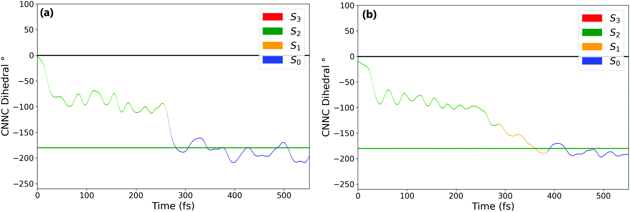
In order to better understand the isomerisation, let us discuss the dynamics in more detail, examining internal coordinates and geometries at which hops between electronic states occur. Fig. 3 shows the changes in the central C–NN–C angle and in the central NN bond length. From these it is clear that the mechanism of isomerisation is rotation-based, with the CNNC dihedral reaching −90° within 50 fs for almost all trajectories. This is in agreement with previous computational studies of the isomerisation mechanism.18,20 There is a clear preference for direction of rotation due to steric hindrance of the phenyl rings, with rotation towards negative dihedral angles preferred. This is defined in previous works as the anticlockwise direction and shown visually in Fig. S2 in the ESI.†![[thin space (1/6-em)]](https://www.rsc.org/images/entities/char_2009.gif) 37 The full inversion mechanism can be rejected, since the CNN angles do not typically exceed 160° and the average CNN angle barely changes (see Fig. S8 in the ESI†) – in the inversion isomerisation mechanism one (or both) of the CNN angles would pass through 180°.
37 The full inversion mechanism can be rejected, since the CNN angles do not typically exceed 160° and the average CNN angle barely changes (see Fig. S8 in the ESI†) – in the inversion isomerisation mechanism one (or both) of the CNN angles would pass through 180°.
 | ||
| Fig. 3 Evolution of selected internal coordinates – (a) and (b) C–NN–C dihedral and (c) and (d) NN bond – throughout the simulations after (a) and (c) nπ* excitation, or (b) and (d) ππ* excitation. Colouring of (a) and (b) represents the active state of each trajectory at each timestep – active state colouring is excluded for visual clarity from figures (c) and (d). Horizontal lines in (a) and (b) indicate the cis (black) and trans (green) isomers. The solid black lines in (c) and (d) represent the average NN bond length across all trajectories. | ||
From examination of some sample isomerising trajectories (of which some typical examples are given as movies in the ESI†), the mechanism can be more clearly understood. Excluding a handful (around 5%) of trajectories which rotate in the unfavourable clockwise direction, the first step that the trajectories follow is a rapid change in the central C–NN–C dihedral, rotating anticlockwise from the starting value of around −3.5° to ca. −90° within the first 50 fs (Fig. 3).
From this point, the ensemble splits into three main groups of trajectories; (i) some trajectories rotate back towards 0 within the next 100 fs and, as a result, reform the cis isomer – these are non-reactive trajectories; (ii) some trajectories continue to rotate past −90° immediately, reaching around −180° in around 150° additional fs to form the trans isomer; and (iii) a smaller number of trajectories oscillate around −90° for some time (>100 fs) after the initial fast rotation to −90°. These trajectories can form either the cis or trans isomer, although the trans isomer is preferentially formed.
While the initial rotation to −90° is the same for both excitations, the differences between the two ensembles of photochromes begin to appear after this point (ca. 50 fs), in the splitting of trajectories into these three categories. More specifically, the major difference is seen in the number of trajectories which pass through −90° and proceed immediately to the trans isomer, versus those which remain around −90° for a significant period of time (>100 fs) – this is visually clear in Fig. 3(a) and (b). The percentage of photochromes that follow each pathway when starting in the nπ* (S1) and the ππ* (S2) states respectively are given in Table 2. These values are obtained by counting the number of trajectories in each pathway (determined by central C–NN–C dihedral) at time 170 fs.
N–C = −90° obtained at time 170 fs
| cis (%) | trans (%) | S2 trapping (%) | |
|---|---|---|---|
| S1(nπ*) excitation | 42 | 37 | 14 |
| S2(ππ*) excitation | 43 | 19 | 31 |
The major difference seen between the dynamics initiated in the two different states is the number of trajectories that remain stuck around −90° instead of continuing rotation to −180° and consequently forming trans-AZB. More than twice as many trajectories are trapped around −90° when starting from the ππ* state, and they are also trapped around −90° for a longer period of time – on average ∼100 fs longer.
We can conclude that the major pathways followed after excitation are the same, with the differences between the two excitations mainly being in the splitting of trajectories, i.e., the percentage of photochromes which follow each pathway. The plot starting in the to ππ* state is also more noisy than starting in the lower energy nπ* state, as expected due to the higher energy of the system. Another major difference between nπ* and ππ* excitations is that the latter is accompanied by a significant activation of the NN stretching mode, not seen in the former; see Fig. 3(c) and (d).
In order to characterise the dynamics relating to the trajectories that follow each of the pathways, the trajectories for the C–NN–C dihedral plots in Fig. 3(a) and (b) are coloured to represent the state that each trajectory is in at each timestep. It can be seen that the trajectories that remain stuck around −90° are mostly in the S2 state. In fact, after S1 excitation, the trajectories ‘trapped’ around −90° for a significant time are those that have undergone a back-hop from S1 → S2 and are in the S2 state around −90°. This ‘trapping’ should therefore be related to the shape of the S2 potential energy surface. By carrying out a fixed geometry scan (Fig. S3 and S4 in the ESI†) along the central C–NN–C coordinate, the shape of the potential energy surfaces in this rotational coordinate was characterised. The shape of these potential energy surfaces support this ‘trapping’, with a minimum in S2 for a dihedral close to −90°, as well as a larger gap between the S2 and S1 surfaces compared to that between the S1 and S0. The molecules that remain around −90° in the S2 state can be interpreted as becoming trapped in a potential well, oscillating around this point in other coordinates. This possibility of trapping after ππ* excitation in a S2 rotational potential well was also reported by Zhu et al.20
On escaping this potential well, the S2 → S1 hops occur at an average C–NN–C dihedral angle of −93.1°, with a minimal spread around this average value – see the distribution of the dihedral of hops in Fig. S10 in the ESI.† The S2 → S1 hops do not generally occur around the optimised S2/S1 conical intersection (CI, geometry given in ESI†) which has a central C–NN–C value of −59.9°, nor around the other optimised S2/S1 CI found by Zhu et al.20 at −132°.
Based on the optimised CIs and on transient absorption data, some others have previously proposed that isomerisation can occur via S2/S1 conical intersections, with the final trans isomer being formed in the S1 state.16,20 We do indeed find this in our simulations, however only for a fraction (8%) of overall photochromes excited to S2. The isomer formed for the trajectories that remain trapped on the S2 surface is mostly determined by the rotational path taken after the ensuing S1 → S0 hop: for 73% of photochromes trapped on S2 (21% of all ππ* trajectories), S1 → S0 hopping occurs almost immediately after S2 → S1. This S1 → S0 hopping also occurs around the same dihedral value, with an average of −93.3°. However, for the remaining 27% of photochromes trapped in S2 (8% of all ππ* trajectories), the S1 → S0 hop does not occur until later in the simulation, when the central C–NN–C dihedral has reached around 180°. The difference between these two cases is illustrated in Fig. 4. In the first case Fig. 4(a), the trajectory spends only 6 fs in the S1 state after S2 → S1 hopping, S1 → S0 hopping occurs almost immediately. However, in the second case Fig. 4(b), the isomerisation has indeed taken place via the S2/S1 conical intersection (which is typically at angles rotated past −90°) and the trans isomer is present in its S1 state. This is consistent with the presence of excited state absorption (ESA) bands attributed to trans-AZB in the study of Quick et al.16 Since for these 8% of overall photochromes the trans isomer formed by photoisomerisation is formed in the nπ* S1 excited state, ESA bands of the trans-AZB would be expected to appear after around 250 fs based on our simulations. This is again closely in line with these experimentally measured ESA bands, which in fact begin to appear at times >200 fs.16
 | ||
| Fig. 4 Example of the two types of trajectory that leave the S2 well after ππ* excitation. (a) Leaves the S2 well via rapid consecutive S2 → S1 → S0 intersections, all located around −90°, (b) leaves the S2 well via S2 → S1 intersection around −90° but isomerises to trans-AZB before S1 → S0 decay. Horizontal lines indicate the cis (black) and trans (green) isomers. | ||
A summary of the important pathways followed by cis-AZB after nπ* and ππ* excitation that have been described in this section is given in Fig. 5, along with the fraction of photochromes which follow each pathway.
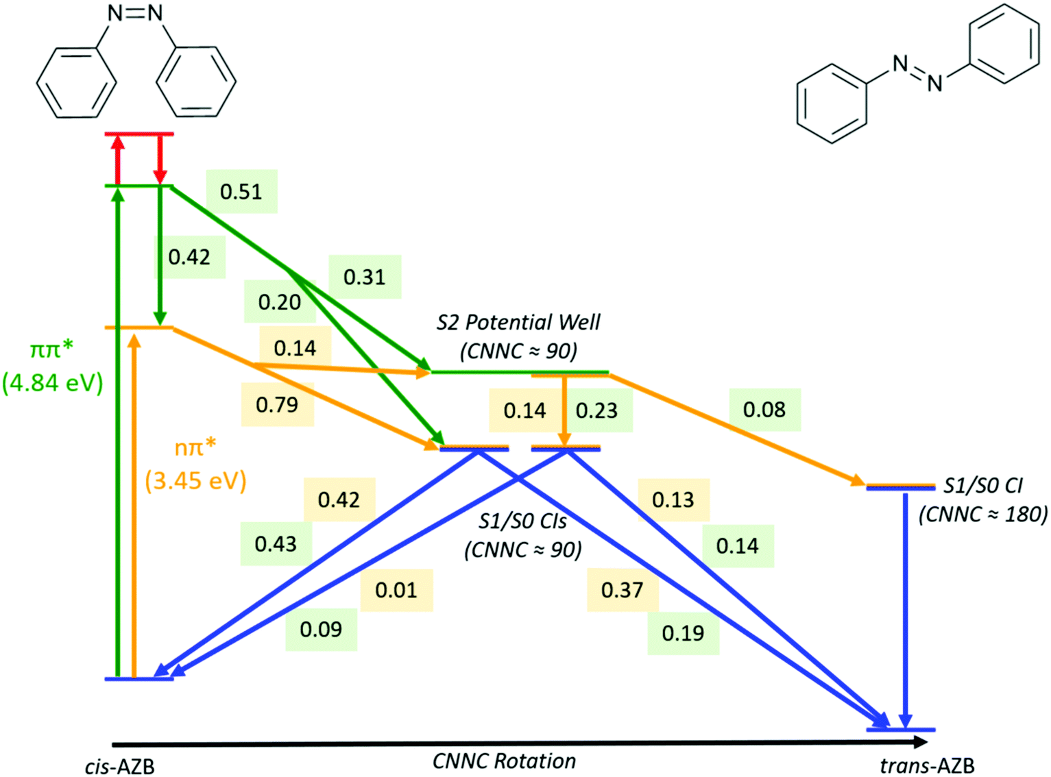 | ||
| Fig. 5 Summary of major pathways, and the fraction of trajectories which follow each pathway, accessible to cis-AZB upon excitation to the nπ* (numbers in yellow) and ππ* (numbers in green) states. | ||
3.3 Quantum yields
N–C angle passes 180°. There are some trajectories that pass through 180° and continue to rotate back to 360°, but in a more realistic simulation energy loss to the solvent/bath would mostly prevent this from happening. We therefore assume that if a value of CNNC = 180° is reached the trajectory can be treated as reactive, forming trans-AZB. This also assigns the few trajectories still trapped in the S2 well at the end of the simulation as cis-AZB – from examination of the evolution of these trajectories, this can be justified as the dihedral angle in all remaining trajectories of this type are in the process of rotating back to cis-AZB. A more detailed validation of the method used to assign reactive versus non-reactive trajectories can be found in the ESI† (Fig. S9).
The calculated quantum yields ϕc→t we therefore obtain from these simulations are 0.57 for the nπ* (S1) excitation, and 0.47 for the ππ* (S2) excitation. These quantum yields are in line with those obtained in the previous computational study of Persico et al.,18 with both quantum yields higher than typically obtained in experiment (see Table 1). The higher quantum yield after nπ* excitation compared to ππ* excitation is successfully reproduced by our simulations. The difference between our two calculated quantum yields is 0.10 only – exciting to the ππ* state only results in a slight reduction in quantum yield. This is in line with the most recent measurements of Ladányi et al., who measured a difference in QYs of 0.11. Our theoretical results therefore support these more recent measurements, rather than the previously accepted quantum yields which showed the quantum yield decreasing by up to a factor of two on exciting to ππ*.
It is noted that the solvent used in experiments is expected to influence the yield of the photoisomerization reaction (see Table 1). While our simulations reproduce quantitatively the difference in QYs between the two excitations, it fails at reproducing the absolute individual QYs of the two excitations. A source of error might be the omission of the solvent in the simulation, but including explicit solvent molecules is beyond the scope of the present study.
The commonly accepted trans → cis mechanism for the reduction of quantum yield is as follows:18,29,30 on exciting to the ππ* (S2) state of trans-AZB, additional vibrational energy is given to the C–NN bending modes. This additional energy allows for S1 → S0 decay through a higher energy section of the S1/S0 intersection seam, located earlier along the central CNNC torsional coordinate. To test if this holds for cis → trans isomerisation, let us look at the geometries at which S1 → S0 hopping occurs according to the surface hop algorithm used – these geometries can be interpreted as the points on the intersection seam at which decay takes place.
Fig. 6 compares the C–NN–C dihedral angle and potential energy of the S1 → S0 hops for both initial excitations. From this figure, it is clear that the S1 → S0 hops are mostly located around −85° after both S1 and S2 excitations, and while the hops after S2 excitation are spread over a larger range of angles, they do not on average occur earlier along the central C–NN–C torsion coordinate.
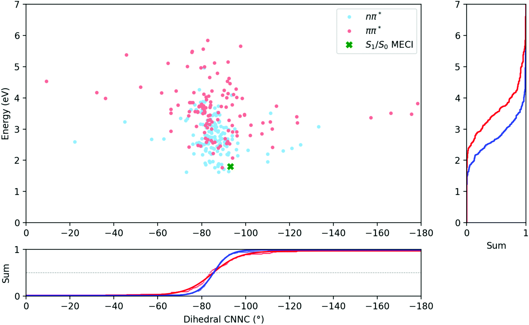 | ||
| Fig. 6 Energies and dihedral angles of the S1 → S0 hopping geometries after excitation to the nπ* (S1) (in blue) and ππ* (S2) (in red) states. The position of the S1/S0 minimum energy conical intersection is indicated by a green cross. | ||
The average dihedral values for the S1 → S0 hops could be obtained by integrating along the dihedral coordinate and fitting to a logistic function, and are listed in Table 3. They are almost perfectly equivalent for both excitations, although the S1/S0 hops do clearly occur at higher potential energies after S2 excitation than after S1. Besides this, the most significant differences are seen in the length of bonds, with bond lengths in general being slightly longer for the ππ* case.
| Property | S1(nπ*) excitation | S2(ππ*) excitation |
|---|---|---|
| Energy (eV) | 2.76 | 3.59 |
| CNNC dihedral (°) | −85.4 | −85.2 |
| Average CNN angle (°) | 123.4 | 124.5 |
| CNN asymmetry (°) | 19.9 | 19.6 |
| NN length (Å) | 1.25 | 1.26 |
| Average CN length (Å) | 1.41 | 1.43 |
| CN difference (Å) | 0.07 | 0.09 |
Unlike for the trans → cis isomerisation, in which the rotation around the central CNNC occurs slowly after excitation, the cis isomer rotation occurs much faster. The previous study by Persico et al. found that after S1 and S2 excitation of trans-AZB, the −90° point was reached after around 400 and 900 fs respectively.18 In comparison, in the same study the −90° point was reached after only 75 and 100 fs for the cis-AZB S1 and S2 excitations respectively.
From scans along the CNNC torsional coordinate (keeping all other coordinates fixed), starting from either the cis or the trans isomer (Fig. S4 in ESI†), the reason for this is clear. The gradient of the slope of the S1 surface along the torsional coordinate is greater for cis-AZB than trans-AZB, and the S2 surface is also sloped towards −90° for cis-AZB, while the S2 state appears at a minimum along the torsional coordinate for trans-AZB. The rotation is therefore significantly faster after S1 excitation for cis versus trans – it takes around 50 fs for cis to rotate to −90° in our simulations. Exciting to S2 also immediately drives the favourable rotation for cis-AZB, while for trans-AZB the rotation is not activated by S2 excitation.
So, instead of bending modes allowing access to higher energy sections of the S1/S0 CI seam while the molecule slowly rotates about the CNNC coordinate, the rotation brings the molecule towards −84° (the average hopping angle) too fast for bending modes to allow access to earlier sections of the CI seam when starting from cis-AZB. As a result the hopping occurs almost exclusively close to the fully twisted geometry (CNNC of ca. −90°) after both nπ* or ππ* excitation.
N–C angles, another mechanism must explain the reduction in yield. As we have been able to reproduce the experimentally measured17 reduction in quantum yield, our simulations should offer physical insight into the mechanism behind this reduction in QY.
As previously described, the main difference between exciting to the nπ* and the ππ* states is the splitting of trajectories after the initial rotation to −90°. In particular, as given in Table 2 the number of trajectories that either remain around −90° for a significant period of time or pass straight through −90° towards the trans isomer is markedly different. The number of trajectories that rotate back to cis-AZB or rotate clockwise is almost identical in both excitation cases.
From Table 2, we can establish that the difference upon exciting to the ππ* state is that there are 16–17% of trajectories, which under nπ* excitation would have immediately formed trans-AZB, that are instead trapped in the S2 well. These trajectories can proceed to either cis-AZB or trans-AZB therefore lowering the quantum yield. However, only 35% of the ππ* trajectories trapped in the well in fact reform cis-AZB, so we would only expect a reduction in QY on ππ* excitation of around 0.05 from this, instead of the calculated reduction of 0.10. There is therefore a second factor which contributes to the QY reduction.
Upon further examination of the trajectories trapped in the S2 well, the 12% that are trapped after nπ* excitation are in fact still associated with the S2 state, and result from back-hops from S1 to S2 around −90°. However, these trajectories leave the S2 well earlier in time than those trapped after ππ* excitation. These trajectories overwhelmingly result in trans-AZB – only 9% of trapped nπ* trajectories form cis-AZB.
So the reduction in QY can be attributed to two factors related to the trapping on the S2 state around −90°: (i) more photochromes are trapped around −90° after ππ* excitation, and (ii) photochromes trapped around −90° after ππ* excitation are roughly 4 times more likely to form cis-AZB than those trapped after nπ* excitation. Since the splitting from the trapping well is different after both excitations, we expect there to be some differences between the two excitation cases in the geometries explored during this pathway. Unfortunately, we do not have enough trajectories that follow this pathway (in particular after nπ* excitation) to be able to carry out a reasonable statistical analysis.
4 Conclusions
We have studied the cis → trans isomerisation mechanism of azobenzene after nπ* and ππ* excitations, using high-level ab initio mixed quantum-classical dynamics, and have demonstrated that our simulations are able to reproduce the trend in quantum yields obtained in the most recent experiments. More specifically, we have determined a decrease in quantum yield of 0.10, from ϕc→t = 0.57 after nπ* excitation to ϕc→t = 0.47 after ππ* excitation. While this is different from previously accepted literature values (as given in Table 1) with measured decreases in quantum yield of up to 0.32,14 it is consistent with the recently measured drop of 0.11.17 Our simulations therefore support these most recent measurements of the quantum yields of azobenzene cis → trans photoisomerisation.We have tested the mechanism for the reduction in quantum yield, as previous studies have typically assumed the reasoning behind lower quantum yields measured at shorter wavelength is the same for both photoisomerisation directions – in other words, it was assumed that the mechanism determined for trans → cis photoisomerisation of AZB also applies to the cis → trans direction.18,24,35 Instead we have found that, unlike for trans → cis photoisomerisation, in the cis → trans case there is no distinct difference between the central C–NN–C angle of the geometries at which S1 → S0 decay occurs when exciting to both nπ* and ππ* states. As a result our calculations do not support the trans → cis mechanism of S1 → S0 decay occurring at higher energy areas of the conical intersection seam, located earlier along the coordinate of rotation about the central C–NN–C dihedral angle. We have explained the absence of this mechanism in cis → trans isomerisation by the immediate activation of the rapid central rotational coordinate for both excitations, reaching ca. −90° too fast to allow for exploration of the S1 → S0 seam along the rotation.
In fact, the rotation occurs on such a timescale that for 51% of photochromes excited to the ππ* state the rotation in fact occurs before S2 → S1 decay, which occurs close to −90°. For the majority of these photochromes the photoreaction product is still determined by the path taken through a subsequent S1 → S0 intersection around −90°, but for 8% of all photochromes excited to ππ* the isomerisation pathway followed involves S1 → S0 decay around 180°, i.e., after isomerisation to trans-AZB. For these 8% of photochromes, the photoisomerisation can conclusively be said to have occurred via the S2 → S1 intersection around −90° as predicted by Quick et al.16
After rejecting the equivalent QY reduction mechanism acting in trans → cis isomerisation, we have instead attributed the reduction of the QY on exciting to the ππ* state compared to nπ* to a potential well on the S2 surface, located around C–NN–C = −90° and accessible after both nπ* and ππ* excitation. Upon leaving this well either cis or trans-AZB may be formed. Two factors relating to this potential well have been found to contribute to the QY reduction: (i) a fraction of photochromes which under nπ* excitation would have exclusively formed trans-AZB were instead trapped in this well after ππ* excitation, and (ii) photochromes in this well had been excited to the ππ* state were also found to be more likely than those excited to the nπ* state to reform cis-AZB upon leaving the well. Our measured reduction in QY of 0.10 thus emerges from the combination of these two factors.
Conflicts of interest
There are no conflicts to declare.Acknowledgements
This work was performed using HPC resources from GENCI-IDRIS (Grant 2020-101353) and CCIPL (Le centre de calcul intensif des Pays de la Loire). I. M. acknowledges thesis funding from the University of Nantes. M. V. acknowledges the Région des Pays de la Loire for financial support through the framework of the PULSAR programme.References
- A. A. Beharry and G. A. Woolley, Chem. Soc. Rev., 2011, 40, 4422–4437 RSC.
- J. Kumar, L. Li, X. L. Jiang, D.-Y. Kim, T. S. Lee and S. Tripathy, Appl. Phys. Lett., 1998, 72, 2096–2098 CrossRef CAS.
- S. Crespi, N. A. Simeth and B. König, Nat. Rev. Chem., 2019, 3, 133–146 CrossRef CAS.
- M. Zhu and H. Zhou, Org. Biomol. Chem., 2018, 16, 8434–8445 RSC.
- M. Böckmann, N. L. Doltsinis and D. Marx, J. Phys. Chem. A, 2010, 114, 745–754 CrossRef PubMed.
- H. Rau and E. Lueddecke, J. Am. Chem. Soc., 1982, 104, 1616–1620 CrossRef CAS.
- I. K. Lednev, T. Q. Ye, L. C. Abbott, R. E. Hester and J. N. Moore, J. Phys. Chem. A, 1998, 102, 9161–9166 CrossRef CAS.
- C. Nonnenberg, H. Gaub and I. Frank, ChemPhysChem, 2006, 7, 1455–1461 CrossRef CAS PubMed.
- H. M. Bandara and S. C. Burdette, Chem. Soc. Rev., 2012, 41, 1809–1825 RSC.
- J. Calbo, C. E. Weston, A. J. White, H. S. Rzepa, J. Contreras-Garca and M. J. Fuchter, J. Am. Chem. Soc., 2017, 139, 1261–1274 CrossRef CAS PubMed.
- G. Zimmerman, L.-Y. Chow and U.-J. Paik, J. Am. Chem. Soc., 1958, 80, 3528–3531 CrossRef CAS.
- S. Malkin and E. Fischer, J. Phys. Chem., 1962, 66, 2482–2486 CrossRef CAS.
- J. Ronayette, R. Arnaud, P. Lebourgeois and J. Lemaire, Can. J. Chem., 1974, 52, 1848–1857 CrossRef CAS.
- P. Bortolus and S. Monti, J. Phys. Chem., 1987, 91, 5046–5050 CrossRef CAS.
- G. Gauglitz and S. Hubig, J. Photochem., 1985, 30, 121–125 CrossRef CAS.
- M. Quick, A. L. Dobryakov, M. Gerecke, C. Richter, F. Berndt, I. N. Ioffe, A. A. Granovsky, R. Mahrwald, N. P. Ernsting and S. A. Kovalenko, J. Phys. Chem. B, 2014, 118, 8756–8771 CrossRef CAS PubMed.
- V. Ladányi, P. Dvořák, J. A. Anshori, Ĺ. Vetráková, J. Wirz and D. Heger, Photochem. Photobiol. Sci., 2017, 16, 1757–1761 CrossRef PubMed.
- C. Ciminelli, G. Granucci and M. Persico, Chem. – Eur. J., 2004, 10, 2327–2341 CrossRef CAS PubMed.
- L. Yu, C. Xu, Y. Lei, C. Zhu and Z. Wen, Phys. Chem. Chem. Phys., 2014, 16, 25883–25895 RSC.
- L. Yu, C. Xu and C. Zhu, Phys. Chem. Chem. Phys., 2015, 17, 17646–17660 RSC.
- C. E. Weston, R. D. Richardson, P. R. Haycock, A. J. White and M. J. Fuchter, J. Am. Chem. Soc., 2014, 136, 11878–11881 CrossRef CAS PubMed.
- D. Bléger, J. Schwarz, A. M. Brouwer and S. Hecht, J. Am. Chem. Soc., 2012, 134, 20597–20600 CrossRef PubMed.
- L. N. Lameijer, S. Budzak, N. A. Simeth, M. J. Hansen, B. L. Feringa, D. Jacquemin and W. Szymanski, Angew. Chem., Int. Ed., 2020, 59, 21663–21670 CrossRef CAS PubMed.
- I. Conti, M. Garavelli and G. Orlandi, J. Am. Chem. Soc., 2008, 130, 5216–5230 CrossRef CAS PubMed.
- Y. Ootani, K. Satoh, A. Nakayama, T. Noro and T. Taketsugu, J. Chem. Phys., 2009, 131, 194306 CrossRef PubMed.
- A. Warshel, Nature, 1976, 260, 679–683 CrossRef CAS PubMed.
- R. S. Liu and A. E. Asato, Proc. Natl. Acad. Sci. U. S. A., 1985, 82, 259–263 CrossRef CAS PubMed.
- H. Rau, in Photochromism, ed. H. Dürr and H. Bouas-Laurent, Elsevier Science, Amsterdam, 2003, pp. 165–192 Search PubMed.
- A. Nenov, R. Borrego-Varillas, A. Oriana, L. Ganzer, F. Segatta, I. Conti, J. Segarra-Marti, J. Omachi, M. Dapor, S. Taioli, C. Manzoni, S. Mukamel, G. Cerullo and M. Garavelli, J. Phys. Chem. Lett., 2018, 9, 1534–1541 CrossRef CAS PubMed.
- F. Aleotti, L. Soprani, A. Nenov, R. Berardi, A. Arcioni, C. Zannoni and M. Garavelli, J. Chem. Theory Comput., 2019, 15, 6813–6823 CrossRef CAS PubMed.
- T. Ishikawa, T. Noro and T. Shoda, J. Chem. Phys., 2001, 115, 7503–7512 CrossRef CAS.
- S. Yuan, Y. Dou, W. Wu, Y. Hu and J. Zhao, J. Phys. Chem. A, 2008, 112, 13326–13334 CrossRef CAS PubMed.
- J. Casellas, M. J. Bearpark and M. Reguero, ChemPhysChem, 2016, 17, 3068–3079 CrossRef CAS PubMed.
- C. Xu, L. Yu, F. L. Gu and C. Zhu, Phys. Chem. Chem. Phys., 2018, 20, 23885–23897 RSC.
- A. Cembran, F. Bernardi, M. Garavelli, L. Gagliardi and G. Orlandi, J. Am. Chem. Soc., 2004, 126, 3234–3243 CrossRef CAS PubMed.
- L. Gagliardi, G. Orlandi, F. Bernardi, A. Cembran and M. Garavelli, Theor. Chem. Acc., 2004, 111, 363–372 Search PubMed.
- M. Pederzoli, J. Pittner, M. Barbatti and H. Lischka, J. Phys. Chem. A, 2011, 115, 11136–11143 CrossRef CAS PubMed.
- L. Ye, C. Xu, F. L. Gu and C. Zhu, J. Comput. Chem., 2020, 41, 635–645 CrossRef CAS PubMed.
- S. Monti, G. Orlandi and P. Palmieri, Chem. Phys., 1982, 71, 87–99 CrossRef CAS.
- Ĺ. Vetráková, V. Ladányi, J. Al Anshori, P. Dvořák, J. Wirz and D. Heger, Photochem. Photobiol. Sci., 2017, 16, 1749–1756 CrossRef PubMed.
- B. O. Roos, P. R. Taylor and P. E. Sigbahn, Chem. Phys., 1980, 48, 157–173 CrossRef CAS.
- B. O. Roos, R. Lindh, P.-Å. Malmqvist, V. Veryazov and P.-O. Widmark, J. Phys. Chem. A, 2004, 108, 2851–2858 CrossRef CAS.
- F. Aquilante, R. Lindh and T. Bondo Pedersen, J. Chem. Phys., 2007, 127, 114107 CrossRef PubMed.
- Y. Harabuchi, M. Ishii, A. Nakayama, T. Noro and T. Taketsugu, J. Chem. Phys., 2013, 138, 064305 CrossRef PubMed.
- K. Andersson, P. A. Malmqvist, B. O. Roos, A. J. Sadlej and K. Wolinski, J. Phys. Chem., 1990, 94, 5483–5488 CrossRef CAS.
- M. Barbatti, M. Ruckenbauer, F. Plasser, J. Pittner, G. Granucci, M. Persico and H. Lischka, Wiley Interdiscip. Rev.: Comput. Mol. Sci., 2014, 4, 26–33 CAS.
- I. F. Galván, M. Vacher, A. Alavi, C. Angeli, F. Aquilante, J. Autschbach, J. J. Bao, S. I. Bokarev, N. A. Bogdanov, R. K. Carlson, L. F. Chibotaru, J. Creutzberg, N. Dattani, M. G. Delcey, S. S. Dong, A. Dreuw, L. Freitag, L. M. Frutos, L. Gagliardi, F. Gendron, A. Giussani, L. González, G. Grell, M. Guo, C. E. Hoyer, M. Johansson, S. Keller, S. Knecht, G. Kovačević, E. Källman, G. Li Manni, M. Lundberg, Y. Ma, S. Mai, J. P. Malhado, P. Å. Malmqvist, P. Marquetand, S. A. Mewes, J. Norell, M. Olivucci, M. Oppel, Q. M. Phung, K. Pierloot, F. Plasser, M. Reiher, A. M. Sand, I. Schapiro, P. Sharma, C. J. Stein, L. K. Sørensen, D. G. Truhlar, M. Ugandi, L. Ungur, A. Valentini, S. Vancoillie, V. Veryazov, O. Weser, T. A. Wesołowski, P.-O. Widmark, S. Wouters, A. Zech, J. P. Zobel and R. Lindh, J. Chem. Theory Comput., 2019, 15, 5925–5964 CrossRef PubMed.
- J. C. Tully, J. Chem. Phys., 1990, 93, 1061–1071 CrossRef CAS.
- S. Hammes-Schiffer and J. C. Tully, J. Chem. Phys., 1994, 101, 4657–4667 CrossRef CAS.
- G. Granucci and M. Persico, J. Chem. Phys., 2007, 126, 134114 CrossRef PubMed.
- The number of trajectories in the S3 state at this time is too low to obtain resolved electronic state populations.
Footnote |
| † Electronic supplementary information (ESI) available: Full active space orbital descriptions; (ii) geometrical coordinates of critical points; (iii) basis set convergence test; (iv) CASSCF vs. CASPT2 energies and state ordering; (v) rigid potential energy scans along central torsional coordinate; (vi) convergence of simulations with number of trajectories; (vii) energy conservation with timestep chosen for trajectories; (viii) additional dynamics plots – electronic populations, internal coordinates, justification of reactive/non-reactive trajectory assignment, and hopping geometry characterisation. (ix) Model trajectories for different pathways. See DOI: 10.1039/d1cp01873f |
| This journal is © the Owner Societies 2021 |