Ambiguities in solvation free energies from cluster-continuum quasichemical theory: lithium cation in protic and aprotic solvents

Abstract

Gibbs free energies for Li⁺ solvation in water, methanol, acetonitrile, DMSO, dimethylacetamide, dimethoxyethane, dimethylformamide, gamma-butyrolactone, pyridine, and sulfolane have been calculated using the cluster-continuum quasichemical theory. With n independent solvent molecules S initial state forming the “monomer” thermodynamic cycle, Li⁺ solvation free energies are found to be on average 14 kcal mol⁻¹ more positive compared to those from the “cluster” thermodynamic cycle where the initial state is the cluster S_n. We ascribe the inconsistency between the “monomer” and “cluster” cycles mainly to the incorrectly predicted solvation free energies of solvent clusters S_n from the SMD and CPCM continuum solvation models, which is in line with the earlier study of Bryantsev et al., J. Phys. Chem. B, 2008, 112, 9709–9719. When experimental-based solvation free energies of individual solvent molecules and solvent clusters are employed, the “monomer” and “cluster” cycles result in identical numbers. The best overall agreement with experimental-based “bulk” scale lithium cation solvation free energies was obtained for the “monomer” scale, and we recommend this set of values. We expect that further progress in the field is possible if (i) consensus on the accuracy of experimental reference values is achieved; (ii) the most recent continuum solvation models are properly parameterized for all solute–solvent combinations and become widely accessible for testing.

---

1 Introduction

Interaction of ions with the solvent is a driving force of many useful transformations involving accumulator charge and discharge cycles, separation chemistry, organic synthesis, dissolution, and pharmacological action of medications.¹ Knowledge of Li⁺ solvation energy in different solvents especially aprotic solvents is crucial for the development and optimization of current and future high capacity energy storage devices such as Li-ion, Li–metal, Li–S, and Li–O₂ batteries.^2–6

For rationalization and careful tuning of these industry-appreciated processes, the quantitative measure of the ionic solute–solvent interplay, the solvation Gibbs free energy of ions, ΔG_solv, is introduced. In contrast to the solvation thermodynamic functions of the neutral solutes accessible via a combination of the sublimation (vaporization) and solubility equilibrium constants from mass-spectrometric, calorimetric and chemical analysis studies, these characteristics of ionic solutes are challenging to obtain.⁷ This is due to the simultaneous presence of both ions and counter-ions in electrolyte solutions.

An indirect way to retrieve the experimental solvation Gibbs free energy of the ion in non-aqueous solvents suggests taking the sum over the following values: (a) Gibbs free energy of ion transfer from water to non-aqueous solution ΔG_tr (W → S); (b) conventional hydration Gibbs free energy of the ion relative to that of the proton for which ΔG^conv_hyd is set to 0 at all temperatures; (c) absolute hydration Gibbs free energy of the proton, ΔG_hyd (H⁺). The ΔG^conv_hyd of anions are precisely measured for equilibria involving strong acids and further utilized to extract these quantities for cations via the solubility products of soluble salts. The ΔG_tr (W → S) and absolute ΔG_hyd (H⁺) require a number of extra approximations to be extracted from the experimental measurements.

Marcus employed the tetraphenyl arsonium tetraphenyl borate (TATB) assumption^8–10 that assigns the same solvation energies to large spherical ions TA⁺ and TB⁻ to derive both the ΔG_tr (W → S) and the absolute proton hydration free energy of −254.3 kcal mol⁻¹ (TATB scale). As the soundness of the TATB assumption is questioned,^11–15 the resulting estimates of Marcus might be insufficiently accurate.

Tissandier and co-workers¹⁶ utilized the so-called cluster pair approximation (CPA),^16,17 claiming that the difference between the solvation free energy of water clusters containing either a single cation or anion disappears as the cluster grows up. This resulted in an absolute hydration free energy of the proton of −266.0 kcal mol⁻¹. Kelly and co-workers¹⁸ using the CPA approximation arrived at −266.1 kcal mol⁻¹ supporting the data of Tissandier et al.¹⁶ The difference of ca. 12 kcal mol⁻¹ between the absolute proton hydration free energy derived with the TATB and CPA approximations is ascribed to the surface potential between gas and liquid. The surface potential exists in the CPA approximation, leading to the “real scale”, and is missing in the TATB assumption, leading to the “bulk scale”. The difference of a few kcal mol⁻¹ between the Gibbs free energy of ion transfer from water to non-aqueous solutions derived by Marcus⁸ on the one hand and Kelly et al.¹⁴ on the other hand is much harder to explain, highlighting the large uncertainties in the available experimental data on solvation free energies of ions.

Approaching the solvation free energies from the theory side has also appeared to be troublesome. Despite the fact that explicit consideration of ion solvation through molecular dynamics simulations in conjunction with free energy methods is scientifically worth,^20–22 this scheme is not a black-box and poses some technical and practical problems. In particular, for reliable solvation free energies, quite accurate long trajectories on large molecular ensembles are mandatory. The standard non-polarizable force fields are not accurate for this purpose in general as they cannot describe charge-transfer interactions properly.^23,24 Custom-built force fields designed for specific solvent–solute combinations are an option; however, their speed is undermined by too long development time. The density functional theory (DFT) and non-empirical ab initio methods are prohibitively expensive and applicable to study only a limited combination of ionic solute–solvent combinations by a few scientific groups with an exceptional computational budget.

Solving the stationary Schrodinger equation for large gas-phase clusters of solvent molecules with and without the incorporated ionic solute is another option to derive the solvation free energy. Assuming that the DFT optimized geometries and frequencies are of good quality,²⁵ very accurate yet computationally efficient local coupled cluster methods^26,27 can be applied in a single-point (SP) fashion to study the clusters of a few thousand atoms. However, identification of either global or the most stable local minima of the solute–solvent or especially solvent clusters is an unworkable task.

The above-mentioned obstacles in explicit theoretical modeling of solvation resulted in the development of implicit solvation models in which the solvent is described as a dielectric medium. Different computational recipes for the calculation of electrostatic and non-electrostatic contributions to solvation open a series of dielectric continuum methods^28–30 such as various implementations of the polarizable continuum model (PCM),^31,32 conductor-like screening model (COSMO),^33–35 solvation model based on density (SMD)³⁶ and its reparameterization,³⁷ generalized Born solvation model SM12,³⁸ Poisson–Boltzmann solvation model,³⁹ composite method for implicit representation of solvent (CMIRS),^40–43 self-consistent continuum solvation (SCCS),^44,45 easy solvation energy (ESE) approach,⁴⁶ extended easy solvation estimation (xESE)⁴⁷ and universal easy solvation evaluation (uESE),⁴⁸ to name a few. Despite the fact that these models were shown to perform reasonably accurate for neutral solutes,^29,49–55 large failures were recorded for solvation of ionic solutes.^56–59

Finally, the performance of implicit solvation models can be further improved (albeit at substantially higher computational costs) via using the so-called hybrid approach which is often referred to as cluster-continuum quasichemical theory or mixed cluster/continuum model and detailed elsewhere.^{11,56,60–66} At first, the model introduces a few explicit solvent molecules around the solute, forming a cluster and mimicking the solute–solvent specific interactions. Then, the whole cluster is immersed in a dielectric continuum to imitate the non-specific solute–solvent interactions. As there are only a few solvent molecules, the conformational issues are not severe, and all essential local minima can be identified. Moreover, reliable ab initio methods can be employed to calculate the cluster formation energies.

Despite the fact that important findings were obtained with the hybrid approach of solvation,^{56–58,64,67–73} the results were shown to be considerably affected by the choice of (a) initial state of the solvent (separate molecules or clusters);^60,61,66 (b) dielectric continuum model;^61,66 (c) electronic structure theory method.⁶² In this work using the cluster/continuum framework, we systematically assess the influence of factors (a)–(c) on the resulting solvation free energies of the lithium cation in a number of protic (water, methanol) and aprotic (acetonitrile, DMSO, dimethylacetamide, dimethoxyethane, dimethylformamide, gamma-butyrolactone, pyridine, sulfolane) solvents. Keen attention was paid to the conformational issues. The obtained results are influential for further development of the cluster continuum solvation models as well as for unraveling the mechanisms of fundamental processes in electrochemical energy storage devices based on lithium.^2,74,75

2 Computational details

2.1 Mixed cluster-continuum model

Depending on the reference state of the solvent molecules, the two concepts of the hybrid solvation model are exploited in the field. The cluster-continuum quasichemical theory (CC-QCT)^56,60,62 of Pliego and co-workers declares that the initial state of the solvent can be described by separate molecules (“monomers”) in the dielectric continuum.

Then, according to the thermodynamic (“monomer”) cycle depicted in Scheme 1, the solvation free energy of an ion forming a strong bond with the surrounding solvent molecules is given via the following equation:

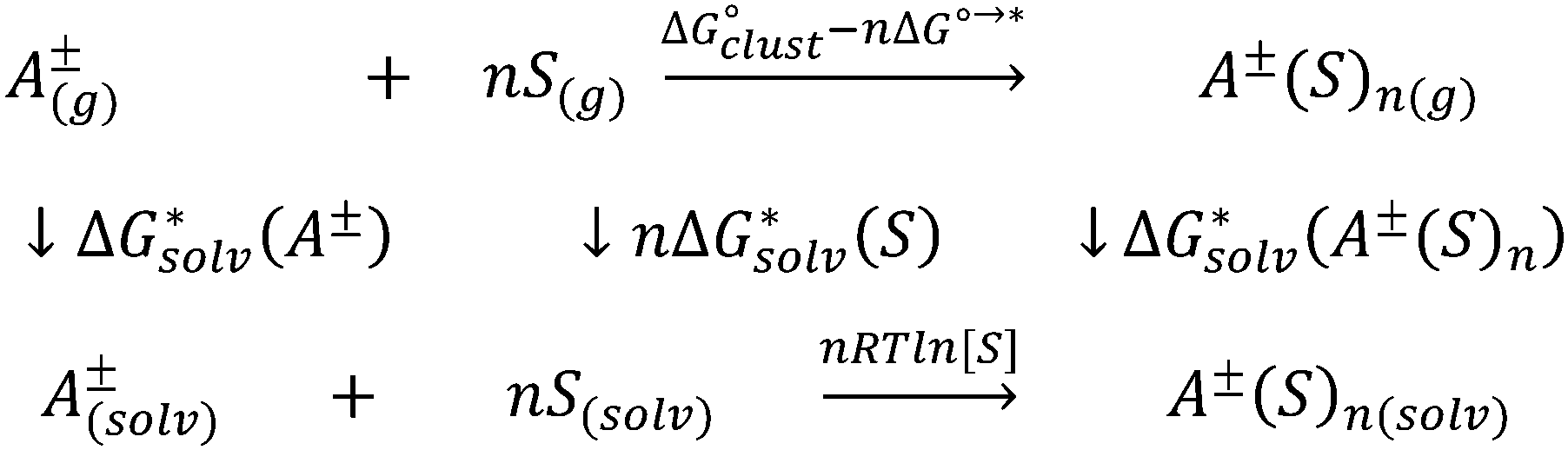Scheme 1 Monomer thermodynamic cycle for calculation of solvation Gibbs free energy of ion A^±.

In this formula, the term is the gas phase Gibbs free energy change of the A^±(S)_n cluster formation from n separate molecules of solvent S and ion A^± with all components in 1 mol L⁻¹ standard state. The 1 mol L⁻¹ can be obtained from 1 atm standard state minus ΔG°^→* correction of 1.89 kcal mol⁻¹ (T = 298.15 K) multiplied n times. The terms and are solvation Gibbs free energies of the solute–solvent cluster and individual solvent molecule as calculated via the continuum approach. The last term, nRT ln[S], contains the solvent density number [S] given in Table 1 for water (H₂O), acetonitrile (MeCN), dimethyl sulfoxide (DMSO), dimethylacetamide (DMA), dimethoxyethane (DME), dimethylformamide (DMF), gamma-butyrolactone (GBL), methanol (MeOH), pyridine (Py), and sulfolane (TMS). The exact number of solvent molecules can be refined variationally.⁵⁶

Table 1 Density number [S] in mol L⁻¹ for solvents considered in this work

Solvent	[S]
H2O	55.34
MeCN	19.12
DMSO	14.08
DMA	10.76
DME	9.64
DMF	12.96
GBL	185.73
MeOH	24.72
Py	12.42
TMS	10.49

---

Opposite to the concept of Pliego and co-workers,^56,60,62 Bryantsev and colleagues^59,61 advocated for using the cluster of solvent molecules as the solvent resting state. Then, according to the thermodynamic (“cluster”) cycle given in Scheme 2, the solvation free energy of the A^± ion can be expressed via the following equation:

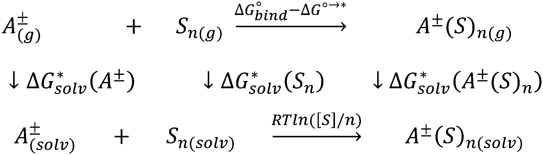Scheme 2 Cluster thermodynamic cycle for calculation of solvation Gibbs free energy of ion A^±.

The 1 atm can be converted to 1 mol L⁻¹ standard state by subtracting from the former the ΔG°^→* correction of 1.89 kcal mol⁻¹ (T = 298.15 K).

The term stands for the solvation free energy of the cluster formed by n molecules of the solvent. It is claimed that the resulting solvation free energies of ions viaeqn (2) should converge with the growth of the number n of explicitly considered solvent molecules. The surface potential is not developed on the small solvent and solute–solvent clusters.^19,76 Nevertheless, the solvation free energies predicted viaeqn (1) are systematically more positive and compared^{11,56,60,62,65} with the “bulk” scale values of Marcus,⁸ and the ΔG_solv calculated viaeqn (2) are more negative and gauged^59,61 against the “real” scale^18,19 quantities, presumably due to the surface potential.

2.2 Determination of the solvent coordination number

The preliminary solvent coordination numbers were estimated from non-periodic molecular dynamics (MD) simulation trajectories. The isokinetic thermostat⁷⁷ at T = 298.15 K as implemented in Priroda 19⁷⁸ was employed on the Li⁺ ion surrounded by 8 solvent molecules. The GGA PBE functional^79,80 was utilized in conjunction with all-electron double-ζ quality basis sets λ₁⁸¹ and the Dyall Hamiltonian⁸² to account for possible scalar relativistic effects. The default adaptively generated PRIRODA grid, corresponding to an accuracy of the exchange–correlation energy per atom (1 × 10⁻⁸ hartree), was utilized for evaluation of the exchange–correlation energy. Default values were used for the self-consistent-field (SCF) convergence. An inspection of the 10 000-step-long trajectory suggests that it is worth considering the following numbers n of solvent molecules in the first coordination sphere of the Li⁺ ion: 4, 5 for MeCN, DMA, water; 3, 4 for DME, pyridine, methanol; 3, 4, 5 for DMSO; 4, 5, 6 for DMF, GBL; and 4 for TMS.

2.3 Conformational issues

The exhausted screening of the most stable local minima of clusters Li⁺(S)_n and (S)_n is an exceptional task requiring a compromise. The standard DFT-D2/3 methods provide a reliable potential energy surface (PES). However, due to high computational costs, these can only be used to sample a limited number of conformers. The standard semiempirical and force field methods are 2–3 orders of magnitude cheaper and can be exploited to cover a substantially larger part of the conformational space, although at the cost of reduced accuracy. In this work, we have prioritized accuracy over completeness and applied the following DFT-D3 based conformational search procedure described below.

For all Li⁺(S)_n and (S)_n clusters and each number of solute molecules n identified in Section 2.2, we performed the 20 000-step-long non-periodic scalar relativistic PBE/λ₁ molecular dynamic simulations with the isokinetic thermostat at T = 298.15 K. From each trajectory we identified 20 most stable, and energetically and structurally diverse structures. Each of 20 structures of Li⁺(S)_n and (S)_n clusters was optimized with the PBE-D3 method,^79,80,83,84 def2-sv(p) basis set^85,86 and with/without the SMD continuum solvation model as implemented in the ORCA 4.2 suite of programs.⁸⁷ Default values were adopted for the self-consistent-field (SCF) and geometry optimization convergence criteria. Numerical integration of the exchange–correlation (XC) terms was performed with the “Grid5 FinalGrid6” option. The resolution-of-identity (RI) approximation was turned on for the sake of computational efficiency. The 20 gas-phase optimized geometries formed the SET_GAS set. Another 20 geometries optimized with the SMD solvation model formed the SET_SMD set. The spatial structures of the most energetically stable species from the SET_GAS and SET_SMD sets for each Li⁺(S)_n and (S)_n cluster were further refined according to the procedure outlined in Section 2.4.

2.4 Geometry optimization and calculation of harmonic frequencies

Within each SET_GAS set, the most stable structure was re-optimized with the PBE-D3 method and minimally diffuse augmented⁸⁸ split valence polarized ma-def2-svp basis set^85,86 as implemented in the ORCA 4.2 collection of computer codes. Each geometry optimization was followed by the calculation of harmonic frequencies. Gas-phase Gibbs free energy correction was calculated within the ideal gas–rigid rotor–harmonic oscillator approximation at 298.15 K in all the cases.

Within each SET_SMD set, the most stable structure was re-optimized according to the identical procedure but with the SMD solvation model turned on. More details on the geometry optimization procedure are provided in the ESI.†

2.5 Single-point energy evaluation

The gas-phase energies necessary for the calculation of and in eqn (1) and (2), were re-evaluated at the optimized geometries by means of the domain-based local-pair natural-orbital coupled-cluster approach with single, double, and improved linear-scaling perturbative triple correction via an iterative algorithm, DLPNO-CCSD(T1),^89–92 method as implemented in the ORCA 4.2 program. The triple-ζ valence correlation consistent polarized basis sets augmented with diffuse functions, aug-cc-pVTZ, were applied to describe (H, C, N, O),⁹³ and S⁹⁴ atoms. According to the literature,^95–98 the sub-valence 1s² electrons on Li were correlated in conjunction with polarized core valence basis sets augmented with diffuse functions, aug-cc-pwCVTZ.⁹⁹

The , and terms in eqn (1) and (2) represent the continuum solvation free energies of molecular clusters and individual solvent molecules calculated within the continuum model. In this formalism, the solvation free energy is obtained as the difference between the molecular electronic energies in the solvent and gas phase. As many continuum solvation models were parameterized using the DFT geometries, energies, and electron densities, we have employed the PBE-D3 method for the calculation of the terms. Since the DFT calculations are known to be less demanding for the basis set size, smaller minimally augmented ma-def2-tzvp^85,86,88 basis sets were employed.

In our first protocol, denoted as SMD_OPT, the terms are calculated as the difference between the PBE-D3 SMD SP energy on the continuum solvent media optimized geometry and the PBE-D3 SP energy on respective gas-phase optimized geometry. In the second approach referred to as SMD_SP, we obtain the terms as the difference between the PBE-D3 SP energies with and without the SMD continuum solvation model on the same gas-phase geometry. If the and contributions to eqn (1) and (2) computed via the SMD_OPT and SMD_SP schemes turn out to be similar, then the expensive geometry optimization and conformational search in the continuum can be avoided.

Our third and fourth protocols termed CPCM_OPT and CPCM_SP were obtained by replacing the SMD solvation model with the conductor-like PCM (CPCM)¹⁰⁰ in the SMD_OPT and SMD_SP protocols, respectively, with all other details remaining unmodified. Unless otherwise noted, the non-electrostatic interactions were not included in the CPCM SP energies (see the ESI† for details).

3 Results and discussion

The Results and discussion section is organized as follows. First, we examine the solvation Gibbs free energy of the Li cation obtained via pure continuum models with no explicit solvent molecules introduced. Second, we discuss the results calculated within the cluster-continuum formalism and compare them with available literature data. Third, we focus on resolving the discrepancies between the “monomer” and “cluster” cycles for the lithium ion solvation free energies. Finally, we propose a set of recommended values.

3.1 Solvation Gibbs free energies from stand-alone continuum models

Fig. 1 and Table S1 (ESI†) open up our discussion and present the lithium cation solvation free energies obtained with pure continuum models. Compared to the “bulk scale” experimental solvation free energies of Marcus, our predicted SMD_SP values turned out to be more positive by 29.7 kcal mol⁻¹ on average. It is noteworthy that these values would be even more positive with respect to the “real” scale. Remarkably, the CPCM_SP strategy produced the absolute solvation free energies, which are substantially closer to respective experimental estimates of Marcus with reasonable MSE/MUE of 2.3/3.7 kcal mol⁻¹.

Fig. 1 Li⁺ solvation Gibbs free energies from pure continuum solvation models against their experimental “bulk” scale counterparts in kcal mol⁻¹.

For both SMD_SP and CPCM_SP strategies, the Pearson correlation coefficient (ρ) between predicted and experimental data was close to zero (see Table S1, ESI†), suggesting no correlation. Indeed, according to continuum solvation models, the lithium cation solvation free energies in MeCN and DMA are practically identical, while experimentally, there is a gap of 12 kcal mol⁻¹. The poor predictive power of stand-alone dielectric solvation models is confirmed by previous reports. In particular, Bryantsev and co-workers⁵⁹ highlighted the inability of the Jaguar Poisson–Boltzmann (PB) solvation model to demonstrate the difference between the MeCN and DMSO lithium solvation free energies captured in the experiment. Noteworthily, their PB solvation free energies turned out to be ca. 20 and 45 kcal mol⁻¹ more negative compared to our CPCM_SP and SMD_SP calculated values, respectively.

To unravel the mismatch between solvation free energies predicted from various continuum models and their experimental counterparts, let us recall the basics of the dielectric model formalism. In practically all continuum models the solvation free energy is split into its electrostatic and non-electrostatic components:

In the case of a spherical ion, within the dielectric continuum model formalism the term is equal to its counterpart from the Born¹⁰¹ formula:

where N_A is the Avogadro constant, z is the ion charge, e is the elementary charge, ε₀ is the vacuum permittivity, r₀ is the effective solute radius, and ε_r is the solvent dielectric constant.

Using the Born formula (4) and the CPCM ORCA 4.2 Li radius of 1.404 Å, we obtained the values identical to the CPCM_SP quantities (see Table S1, ESI†). To unravel the difference between the SMD_SP and CPCM_SP strategies, we first subtracted the non-electrostatic contribution from the SMD_SP solvation energies to arrive at SMD_SP (EL) parts (see Table S1, ESI†). The SMD_SP (EL) values turned out to be equal to the Born formula quantities obtained for the SMD Li radius of 1.82 Å. This means that the substantial difference between the SMD_SP and CPCM_SP predicted solvation free energies is originated from different atomic radii used for calculation of . The term calculated within the SMD formalism for the Li⁺ ion in the solvents considered in this work turned out to be 1–2 kcal mol⁻¹ only. Furthermore, it has to be noted that the thus obtained SMD term is not accurate as it contains only the cavitation-like contribution proportional to the molecular surface tension σ^[M]. Other important non-electrostatic terms, apparently responsible for the difference between the MeCN and DMSO solvents, are not calculated as atomic surface tension parameters are not available for lithium in the original SMD article.³⁶ Finally, using the Born formula and the lithium radius of 1.226 Å mentioned by Bryantsev and co-workers⁵⁹ as Jaguar PB default, we arrived at solvation free energies of Li⁺ that are within 1–2 kcal mol⁻¹ from their Jaguar PB values. As for the choice of the Li⁺ radius, we find the CPCM default reasonable as it is fairly close to the isoelectronic He atom van-der-Waals radius of 1.40 Å recommended by Bondi.¹⁰² Hence, the disagreement between the CPCM_SP and experimental solvation free energies is due to non-electrostatic terms such as cavitation, dispersion, repulsion, and specific Li ← S interactions. The SMD Li⁺ radius corresponds to the neutral lithium atom¹⁰² and is too large. In contrast, the Jaguar PB default Li⁺ radius is too small.

All these findings indicate that pure continuum solvation models are quite promising for the calculation of the solvation free energies of ions if respective radii are carefully chosen and non-electrostatic terms are properly taken care of. It has to be underlined that reasonable solvation free energies with these models can be achieved at the cost of gas-phase SP calculation without tedious manual work as in the “hybrid” approach discussed vide infra.

3.2 Solvation Gibbs free energies from the cluster-continuum approach

Fig. 2 represents the solvation free energies calculated via the “monomer” and “cluster” cycles, respectively. Precise numbers forming the basis of Fig. 2 can be extracted from Tables S2 and S3 (ESI†).

Fig. 2 Monomer and cluster cycle Li⁺ solvation Gibbs free energies.

For the “monomer” cycle, the average span between the minimum and maximum Li⁺ solvation free energies obtained with the continuum model strategies tested in this work amounts to 4.5 kcal mol⁻¹. Similarly, for the “cluster” cycle the average difference between the predicted minimum and maximum solvation free energies of the Li cation is 4.3 kcal mol⁻¹. These variations in solvation free energies due to differences in continuum models are substantially smaller compared to the variations in the stand-alone SMD and CPCM predicted solvation Gibbs free energies (see Fig. 1). Hence, the introduction of the explicit solvent molecules in the cluster-continuum approach evens out the difference between the pure continuum models. The average difference between the SMD_OPT and SMD_SP predicted Li⁺ solvation free energies amounts to 0.8 and 1.0 kcal mol⁻¹ for the “monomer” and “cluster” cycles, respectively. Similarly, the average deviation between the CPCM_OPT and CPCM_SP predicted values is equal to 0.7 and 1.0 kcal mol⁻¹ for the “monomer” and “cluster” cycles. These observations suggest that computationally quite expensive conformational search and geometry optimization with continuum solvation effects included can, in general, be avoided. Finally, the average difference between the SMD_OPT and CPCM_OPT lithium cation solvation free energies amounts to 3.9 and 3.3 kcal mol⁻¹ for the “monomer” and “cluster” cycles, respectively. Similarly, the average difference between the SMD_SP and CPCM_SP values is equal to 3.5 and 3.2 kcal mol⁻¹ for the “monomer” and “cluster” cycles. Analysis suggests that the average difference of 3–4 kcal mol⁻¹ between the SMD and CPCM predictions originates from (i) the use of different atomic radii in the calculation of the electrostatic part of solvation free energies; (ii) missing non-electrostatic interactions in the default CPCM ORCA 4.2 implementation (see Section 2.5).

The lowest Li⁺ solvation free energies obtained within the “monomer” cycle suggest considering the number of explicit solvent molecules n = 3 for DME and n = 4 for all other solvents in this work. According to the “cluster” cycle, slightly more negative solvation free energies can be obtained for larger numbers n for some combinations of solvents and continuum solvation model strategies. However, the found energy drop of 1–2 kcal mol⁻¹ was not substantial, concluding that the results are starting to converge for the numbers of explicit solvent molecules already found for the “monomer” cycle. For these reasons, we used the “monomer” cycle numbers n for the “cluster” cycle as well. Moreover, these numbers n were in agreement with the “cluster” cycle study of Bryantsev and co-workers.⁵⁹ For the sake of consistency, we first compare our predicted “monomer” cycle solvation free energies with their literature counterparts obtained for the same cycle. Afterward, we proceed to the “cluster” model results. All individual components of eqn (1) and (2) needed for the calculation of solvation free energies via both cycles are listed in Tables S4 and S5 (ESI†).

Using the “monomer” cycle, Carvalho and Pliego⁶² reported a Li⁺ bulk solvation free energy in water of −116.1 kcal mol⁻¹ for Li⁺(H₂O)₄ coordination. Our predicted are in reasonable agreement with this value, and all fall in the range between −115.8 and −117.5 kcal mol⁻¹ depending on the particular solvation model. The same authors predict the in acetonitrile of −120.6 kcal mol⁻¹. This number is more negative than our calculated values ranging from −110.5 to −115.2 kcal mol⁻¹. This mismatch arises from our predicted being 5.9 kcal mol⁻¹ more negative due to considering CH₃-related vibrational modes in Li⁺(MeCN)₄ as free rotors by Carvalho and Pliego. For Li⁺ solvation free energy in DMSO, the authors report of −123.6 kcal mol⁻¹. It is reasonably close to our CPCM_OPT and CPCM_SP predictions of −122.7 and −121.2 kcal mol⁻¹, and more positive compared to our SMD_OPT and SMD_SP estimates of −128.8 and −127.8 kcal mol⁻¹. Pliego and Miguel⁶⁵ reported a free energy of in MeOH of −118.1 kcal mol⁻¹. This value is reasonably close to our predictions ranging from −115.6 to −118.5 kcal mol⁻¹, depending on the continuum solvation model strategy. Apart from small deviations in the term, the mismatch in Li⁺ solvation free energies in methanol arises from our calculated being 3.8 kcal mol⁻¹ more positive compared to the corresponding term in ref. 65.

Bryantsev and co-workers exploited the “cluster” cycle to obtain lithium cation solvation free energies in a number of solvents.⁵⁹ For the MeCN solvent the authors suggest a lithium cation solvation free energy of −121.7 kcal mol⁻¹. Our “cluster” model results are systematically more negative and range from −128.3 to −132.9 kcal mol⁻¹. Similarly, for the Li⁺ solvation process in DMA in the form of Li⁺(DMA)₄ the authors derived a Gibbs free energy of −131.5 kcal mol⁻¹. According to our calculations, in DMA for n = 4 varies from −134.0 to −140.1 kcal mol⁻¹ depending on the particular continuum solvation model. For Li⁺ solvation in DME in the form of Li⁺(DME)₃, Bryantsev and co-workers calculated a solvation free energy of −128.3 kcal mol⁻¹. Our predictions for this number of explicitly coordinated DME molecules range from −133.3 to −138.3 kcal mol⁻¹. Finally, for Li⁺ solvation in DMSO in the form of Li⁺(DMSO)₄, the authors find a Gibbs free energy of −133.1 kcal mol⁻¹. Again, for the number n = 4 of explicitly coordinated DMSO molecules, we predict Li⁺ solvation Gibbs free energies ranging from −138.5 to −143.7 kcal mol⁻¹. Interestingly, the best agreement between our predicted solvation free energies and their counterparts from the work of Bryantsev and co-workers was achieved for the CPCM_SP results as this continuum model results in the most positive values.

Unfortunately, Bryantsev and co-workers did not provide the Cartesian coordinates as well as electronic and solvation free energies of all individual species studied in their work, making it difficult to identify the origin of disagreement with our predicted values via the same cycle. We assume, nevertheless, that the main source of discrepancies is due to a contribution from the term. While we utilized the default radii from the continuum solvation model, the authors of ref. 59 scaled the radii to reproduce experimental solvation free energies of some neutral molecules.

Irrespective of the continuum model, the “monomer” cycle lithium cation solvation free energies obtained in this work are found to be on average 14 kcal mol⁻¹ more positive compared to those from the “cluster” cycle. The other research groups report similar deviations between the values derived from these cycles.^60,61,66 The origin of the difference between the solvation Gibbs free energies obtained from the “monomer” and “cluster” cycles is to be discussed in the next section.

3.3 The origin of the discrepancies between the solvation Gibbs free energies from “monomer” and “cluster” cycles

If the computational chemistry methods were perfect, the difference between the solvation Gibbs free energies of ions obtained via the “monomer” and “cluster” cycles would not exist. It is possible to show⁶¹ that according to the thermodynamic cycle depicted in Scheme 3, the solvation free energy of solvent clusters can be obtained via the following equation:

Scheme 3 Thermodynamic cycle of solvent cluster formation.

Replacing the term in eqn (2) with (5) should result in eqn (1). However, according to our calculations, due to inaccuracies in approximations described in Section 2, the predicted solvation free energies of solvent clusters (S)_n from all considered continuum models deviate substantially from their counterparts calculated viaeqn (5) (see Fig. 3 and Table S6 (ESI†)). This turns eqn (5) into an inequation leading to documented discrepancies between the solvation Gibbs free energies of the lithium cation predicted via the “monomer” and “cluster” cycles.

Fig. 3 Difference between obtained from the continuum model (CM) and their eqn (5) counterparts. CM stands for the continuum model.

There are only three reasons for eqn (5) values not matching their counterparts from continuum models:

(1) The gas-phase Gibbs free energy of solvent cluster formation from individual solvent molecules, , is inaccurate.

(2) The solvation free energies of individual solvent molecules in eqn (5) predicted with continuum models are erroneous.

(3) The solvation free energies of solvent clusters obtained via continuum models and utilized in eqn (1) and (2), and left-hand side of eqn (5) are unreliable.

Experience suggests that reaction energies/enthalpies from the DLPNO-CCSD(T)/aug-cc-p(wC)VTZ//PBE-D3/ma-def2-svp protocol should be quite accurate.^103,104 Due to a wealth of low-lying frequencies in the solvent clusters, the entropy changes calculated for gas-phase reaction in Scheme 3 could be less reliable, yet leading to total errors in of only a few kcal mol⁻¹. For these reasons, the predicted in this work and utilized in eqn (5) are most likely correct with potential inaccuracies of 2–3 kcal mol⁻¹. Hence, explanation (1) above can be ruled out.

Further, we derived the experimental Gibbs free energies of self-solvation of all solvents from the available^105–111 pressure of saturated vapors:

The experimental are compared with their continuum solvation model equivalents in Fig. 4 and Table S7 (ESI†). The MUE deviations are 0.7, 0.6, and 1.1 kcal mol⁻¹ for SMD_OPT, SMD_SP, and CPCM_OPT/CPCM_SP protocols, respectively. The MSEs are found to be low and all in the range from −0.3 to −0.6 kcal mol⁻¹, and cannot be responsible for large systematic deviations reported in Fig. 3 and Table S6 (ESI†). Hence, explanation (2) can be eliminated as well.

Fig. 4 Self-solvation Gibbs free energies from continuum solvation models against their experimental counterparts.

For these reasons, we conclude that the free energies from the considered continuum solvation models are erroneous and entirely accountable for the mismatch between the lithium ion solvation free energies calculated via the “monomer” and “cluster” cycles. To illustrate the degree of incorrectness, we compare in Fig. 5 and Table S8 (ESI†) the continuum models with their eqn (5) counterparts obtained via a combination of the DLPNO-CCSD(T) and experimental from Fig. 4 and Table S7 (ESI†). These findings are in line with the previous report of Bryantsev et al.⁶¹ on the solvation of the proton and Cu²⁺ cation in water.

Fig. 5 Eqn (5) calculated from the DLPNO-CCSD(T) and experimental against their counterparts from continuum solvation models in kcal mol⁻¹.

3.4 Solvation Gibbs free energies from the experimental-based monomer/cluster cycle

Given that the origin of disagreement between the “monomer” and “cluster” has been identified, one might consider another approach to the most reliable lithium cation solvation free energy. In the “monomer” cycle eqn (1), one could use the experimental solvation free energy of solvent S listed in Table S7 (ESI†) and obtained viaeqn (6) and its saturated vapor pressure. Similarly, in the “cluster” cycle eqn (2) one could operate with eqn (5) solvation free energies of (S)_n listed in Table S8 (ESI†) that are in turn obtained with experimental eqn (6). We refer to this strategy as the “experimental-based monomer/cluster” cycle. Thus obtained are identical for both “monomer” and “cluster” cycle equations and are plotted in Fig. 6 and listed in Table S9 (ESI†). As contemporary computational chemistry methods result in accurate , and , the “experimental-based monomer/cluster” cycle will be as accurate as from continuum models. As non-electrostatic interactions are missing in our CPCM-based strategies, we expect the SMD_OPT and SMD_SP strategies to provide more realistic and in the “experimental-based monomer/cluster” cycle.

Fig. 6 Experimental-based monomer/cluster (EB MC) Li⁺ solvation Gibbs free energies.

3.5 Recommended values

Bryantsev and co-workers⁶¹ suggest the better performance of the “cluster” cycle for calculating solvation free energies of ions due to favorable compensation of errors for calculation of properties of the clusters of similar size, A^±(S)_n and (S)_n. However, it is still open to discussion whether cancellation of errors occurs,⁶⁰ for instance, between the continuum model solvation free energies of Li⁺(S)_n and (S)_n. While the former species are relatively stable and do not imply a free exchange of ligand S with the surrounding solvent molecules, it is not the case for the latter species. Moreover, the conformational space of the (S)_n species is substantially more difficult to explore than that of Li⁺(S)_n. This results in higher chances to identify the low energy conformer for Li⁺(S)_n but not for (S)_n breaking the error compensation.

In our opinion, a reasonable way to define a set of recommended values is to compare our predicted values with their experimental counterparts reported by Marcus for bulk solvation⁸ and available for MeCN, DMA, DMF, DMSO, H₂O, MeOH, and TMS solvents. The deviations between obtained via different strategies and their Marcus “bulk” scale counterparts in the form of ρ, MUE, and MSE are given in Fig. 7a–c and Table S10 (ESI†). According to Fig. 7a–c the lowest MUE and MSE and the highest ρ were obtained for the monomer cycle that inclines us to recommend these values. The “monomer” cycle performance is followed closely by that of the experimental-based monomer/cluster cycle. The worst performance was detected for the cluster cycle regardless of the number of explicitly coordinated solvent molecules considered. The large negative MSE values obtained for the “cluster” cycle can be reduced if using the CPA proton scale of Kelly et al.^18,19 and correcting the Marcus⁸ experimental numbers accordingly. The somewhat lower ρ values obtained for the cluster cycle are harder to explain.

Fig. 7 (a) The Pearson correlation coefficient (ρ) between predicted from different schemes and their experimental-based “bulk” scale counterparts of Marcus. (b) Mean unsigned error (MUE) of predicted from different schemes with respect to their experimental-based “bulk” scale counterparts of Marcus. (c) Mean signed error of predicted from different schemes with respect to their experimental-based “bulk” scale counterparts of Marcus. EB M/C stands for experimental-based monomer/cluster cycle.

4 Conclusions

The cluster-continuum quasichemical theory (CC-QCT) has been employed to study the lithium cation solvation in a number of protic and aprotic solvents. In line with earlier reports, the calculated Li⁺ solvation Gibbs free energies turned out to be highly dependent on the choice of the particular continuum solvation model and the initial state of the solvent. With n independent solvent molecules S initial state, forming the “monomer” cycle, Li⁺ solvation free energies are found to be on average 14 kcal mol⁻¹ more positive compared to those from the “cluster” cycle where the initial state is the cluster (S)_n. The difference between the continuum SMD and CPCM models utilized in this work is due to (i) the use of different atomic radii in the calculation of the electrostatic part of solvation free energies; (ii) missing non-electrostatic interactions in the default CPCM ORCA 4.2 implementation. Using the additional thermodynamic cycle of solvent cluster formation as in ref. 61, we show that the difference between the “monomer” and “cluster” cycles predicted values is entirely due to incorrect too positive solvation free energies of solvent clusters from SMD and CPCM continuum models utilized in this work. When experimental-based solvation free energies of individual solvent molecules and solvent clusters are utilized, the “monomer” and “cluster” cycles result in identical values. We refer to this set of new values and the corresponding approach as the “experimental-based monomer/cluster” (EB MC) cycle. The best agreement with experimental-based “bulk” scale lithium cation solvation free energies of Marcus was documented for the “monomer” cycle, making it possible to recommend this set of values. Somewhat more significant errors were obtained for the “experimental-based monomer/cluster” cycle lithium cation solvation free energies that are as accurate as the values from continuum models taking no advantage from error compensation. Finally, the largest deviations were observed for the “cluster” cycle predictions. We ascribe this to substantially more accurate continuum model solvation free energies of Li⁺(S)_n species compared to that of (S)_n clusters that breaks error cancellation. We expect that further progress in the field is possible if (i) consensus on the accuracy of experimental reference values is achieved; (ii) the most recent continuum solvation models are properly parameterized for all solute/solvent combinations and become widely accessible for testing.

Author contributions

The manuscript was written through contributions of all authors.

Conflicts of interest

There are no conflicts to declare.

Acknowledgements

We gratefully acknowledge Dr Dmitry I. Sharapa, Institute of Catalysis Research and Technology, Karlsruhe Institute of Technology (KIT), Germany; Dr Denis S. Tikhonov, Deutsches Elektronen-Synchrotron (DESY), Hamburg, Germany; Dr Alexander Genaev, N. N. Vorozhtsov Novosibirsk Institute of Organic Chemistry SB RAS, Novosibirsk, Russia, for helpful discussions. We also acknowledge the anonymous reviewers of this work for their useful comments and suggestions. This work was financially supported by the Russian Science Foundation (project 19-43-04112). L. C. gratefully acknowledges the financial support from King Abdullah University of Science and Technology (KAUST). For computer time, this research used the resources of the Supercomputing Laboratory at King Abdullah University of Science and Technology (KAUST) in Thuwal, Saudi Arabia.

Notes and references

1. Y. Marcus, Ions in Solution and their Solvation, John Wiley & Sons, Ltd, Hoboken, New Jersey, 2015, pp. 247–283.
2. W.-J. Kwak, Rosy, D. Sharon, C. Xia, H. Kim, L. R. Johnson, P. G. Bruce, L. F. Nazar, Y.-K. Sun, A. A. Frimer, M. Noked, S. A. Freunberger and D. Aurbach, Chem. Rev., 2020, 120, 6626–6683.
3. L. Kong, L. Yin, F. Xu, J. Bian, H. Yuan, Z. Lu and Y. Zhao, J. Energy Chem., 2021, 55, 80–91.
4. K. Xu, Chem. Rev., 2004, 104, 4303–4418.
5. D. M. Seo, S. Reininger, M. Kutcher, K. Redmond, W. B. Euler and B. L. Lucht, J. Phys. Chem. C, 2015, 119, 14038–14046.
6. S. Han, Sci. Rep., 2019, 9, 5555.
7. P. Hunenberger and M. Reif, Single-Ion Solvation, The Royal Society of Chemistry, Cambridge, UK, 2011.
8. Y. Marcus, Ions in Solution and their Solvation, John Wiley & Sons, Ltd, Hoboken, New Jersey, 2015, pp. 107–155.
9. Y. Marcus, J. Chem. Soc., Faraday Trans. 1, 1987, 83, 2985–2992.
10. Y. Marcus, G. Hefter and T. Chen, J. Chem. Thermodyn., 2000, 32, 639–649.
11. E. Westphal and J. R. Pliego, J. Chem. Phys., 2005, 123, 74508.
12. R. Schurhammer and G. Wipff, THEOCHEM, 2000, 500, 139–155.
13. T. T. Duignan, M. D. Baer and C. J. Mundy, J. Chem. Phys., 2018, 148, 222819.
14. M. Leśniewski and M. Śmiechowski, J. Chem. Phys., 2018, 149, 171101.
15. T. P. Pollard and T. L. Beck, J. Chem. Phys., 2018, 148, 222830.
16. M. D. Tissandier, K. A. Cowen, W. Y. Feng, E. Gundlach, M. H. Cohen, A. D. Earhart, J. V. Coe and T. R. Tuttle, J. Phys. Chem. A, 1998, 102, 7787–7794.
17. J. V. Coe, Int. Rev. Phys. Chem., 2001, 20, 33–58.
18. C. P. Kelly, C. J. Cramer and D. G. Truhlar, J. Phys. Chem. B, 2006, 110, 16066–16081.
19. C. P. Kelly, C. J. Cramer and D. G. Truhlar, J. Phys. Chem. B, 2007, 111, 408–422.
20. B. D. Kelly and W. R. Smith, J. Chem. Theory Comput., 2020, 16, 1146–1161.
21. K. Leung, S. B. Rempe and O. A. von Lilienfeld, J. Chem. Phys., 2009, 130, 204507.
22. T. T. Duignan, M. D. Baer, G. K. Schenter and C. J. Mundy, Chem. Sci., 2017, 8, 6131–6140.
23. F. Jensen, Introduction to Computational Chemistry, Wiley, Chichester, England, 2nd edn, 2016.
24. H. Zhang, Y. Jiang, H. Yan, Z. Cui and C. Yin, J. Chem. Inf. Model., 2017, 57, 2763–2775.
25. W. Koch and M. C. Holthausen, A Chemist's Guide to Density Functional Theory, WILEY-VCH Verlag GmbH, Weinheim, 2nd edn, 2001.
26. F. Neese, A. Hansen and D. G. Liakos, J. Chem. Phys., 2009, 131, 064103.
27. C. Hampel and H. J. Werner, J. Chem. Phys., 1996, 104, 6286–6297.
28. J. Tomasi and M. Persico, Chem. Rev., 1994, 94, 2027–2094.
29. J. Tomasi, B. Mennucci and R. Cammi, Chem. Rev., 2005, 105, 2999–3093.
30. J. M. Herbert, Wiley Interdiscip. Rev.: Comput. Mol. Sci., 2021, e1519.
31. G. Scalmani and M. J. Frisch, J. Chem. Phys., 2010, 132, 114110.
32. J. B. Foresman, T. A. Keith, K. B. Wiberg, J. Snoonian and M. J. Frisch, J. Phys. Chem., 1996, 100, 16098–16104.
33. A. Klamt and G. Schüürmann, J. Chem. Soc., Perkin Trans. 2, 1993, 799–805.
34. A. Klamt, Wiley Interdiscip. Rev.: Comput. Mol. Sci., 2018, 8, e1338.
35. V. Barone, M. Cossi and J. Tomasi, J. Chem. Phys., 1997, 107, 3210–3221.
36. A. V. Marenich, C. J. Cramer and D. G. Truhlar, J. Phys. Chem. B, 2009, 113, 6378–6396.
37. S. Mirzaei, M. V. Ivanov and Q. K. Timerghazin, J. Phys. Chem. A, 2019, 123, 9498–9504.
38. A. V. Marenich, C. J. Cramer and D. G. Truhlar, J. Chem. Theory Comput., 2013, 9, 609–620.
39. C. J. Stein, J. M. Herbert and M. Head-Gordon, J. Chem. Phys., 2019, 151, 224111.
40. A. Pomogaeva and D. M. Chipman, J. Phys. Chem. A, 2013, 117, 5812–5820.
41. A. Pomogaeva and D. M. Chipman, J. Chem. Theory Comput., 2014, 10, 211–219.
42. A. Pomogaeva and D. M. Chipman, J. Phys. Chem. A, 2015, 119, 5173–5180.
43. Z.-Q. You and J. M. Herbert, J. Chem. Theory Comput., 2016, 12, 4338–4346.
44. O. Andreussi, I. Dabo and N. Marzari, J. Chem. Phys., 2012, 136, 64102.
45. C. Dupont, O. Andreussi and N. Marzari, J. Chem. Phys., 2013, 139, 214110.
46. A. A. Voityuk and S. F. Vyboishchikov, Phys. Chem. Chem. Phys., 2019, 21, 18706–18713.
47. A. A. Voityuk and S. F. Vyboishchikov, Phys. Chem. Chem. Phys., 2020, 22, 14591–14598.
48. S. F. Vyboishchikov and A. A. Voityuk, J. Comput. Chem., 2021, 1–11.
49. C. C. Zanith and J. R. Pliego, J. Comput.-Aided Mol. Des., 2015, 29, 217–224.
50. A. V. Marenich, C. J. Cramer and D. G. Truhlar, J. Phys. Chem. B, 2009, 113, 4538–4543.
51. A. Klamt, B. Mennucci, J. Tomasi, V. Barone, C. Curutchet, M. Orozco and F. J. Luque, Acc. Chem. Res., 2009, 42, 489–492.
52. Y. Minenkov, G. Occhipinti and V. R. Jensen, J. Phys. Chem. A, 2009, 113, 11833–11844.
53. E. B. Stukalin, M. V. Korobov and N. V. Avramenko, J. Phys. Chem. B, 2003, 107, 9692–9700.
54. A. C. Chamberlin, C. J. Cramer and D. G. Truhlar, J. Phys. Chem. B, 2008, 112, 8651–8655.
55. J. Zhang, H. Zhang, T. Wu, Q. Wang and D. van der Spoel, J. Chem. Theory Comput., 2017, 13, 1034–1043.
56. J. R. Pliego and J. M. Riveros, J. Phys. Chem. A, 2001, 105, 7241–7247.
57. J. R. Pliego and J. M. Riveros, J. Phys. Chem. A, 2002, 106, 7434–7439.
58. J. Li, C. L. Fisher, J. L. Chen, D. Bashford and L. Noodleman, Inorg. Chem., 1996, 35, 4694–4702.
59. D. G. Kwabi, V. S. Bryantsev, T. P. Batcho, D. M. Itkis, C. V. Thompson and Y. Shao-Horn, Angew. Chem., Int. Ed., 2016, 55, 3129–3134.
60. J. R. Pliego and J. M. Riveros, Wiley Interdiscip. Rev.: Comput. Mol. Sci., 2020, 10, e1440.
61. V. S. Bryantsev, M. S. Diallo and W. A. Goddard III, J. Phys. Chem. B, 2008, 112, 9709–9719.
62. N. F. Carvalho and J. R. Pliego, Phys. Chem. Chem. Phys., 2015, 17, 26745–26755.
63. P. Grabowski, D. Riccardi, M. A. Gomez, D. Asthagiri and L. R. Pratt, J. Phys. Chem. A, 2002, 106, 9145–9148.
64. D. Asthagiri, L. R. Pratt and H. S. Ashbaugh, J. Chem. Phys., 2003, 119, 2702–2708.
65. J. R. Pliego and E. L. M. Miguel, J. Phys. Chem. B, 2013, 117, 5129–5135.
66. L. Tomaník, E. Muchová and P. Slavíček, Phys. Chem. Chem. Phys., 2020, 22, 22357–22368.
67. C.-G. Zhan and D. A. Dixon, J. Phys. Chem. B, 2003, 107, 4403–4417.
68. A. S. McNeill, C.-G. Zhan, A. M. Appel, D. M. Stanbury and D. A. Dixon, J. Phys. Chem. A, 2020, 124, 6084–6095.
69. R. L. Martin, P. J. Hay and L. R. Pratt, J. Phys. Chem. A, 1998, 102, 3565–3573.
70. D. Asthagiri, L. R. Pratt, M. E. Paulaitis and S. B. Rempe, J. Am. Chem. Soc., 2004, 126, 1285–1289.
71. M. Uudsemaa and T. Tamm, J. Phys. Chem. A, 2003, 107, 9997–10003.
72. M. Uudsemaa and T. Tamm, Chem. Phys. Lett., 2004, 400, 54–58.
73. C.-G. Zhan and D. A. Dixon, J. Phys. Chem. A, 2001, 105, 11534–11540.
74. T. Liu, J. P. Vivek, E. W. Zhao, J. Lei, N. Garcia-Araez and C. P. Grey, Chem. Rev., 2020, 120, 6558–6625.
75. T. Kim, W. Song, D.-Y. Son, L. K. Ono and Y. Qi, J. Mater. Chem. A, 2019, 7, 2942–2964.
76. A. A. Isse and A. Gennaro, J. Phys. Chem. B, 2010, 114, 7894–7899.
77. D. N. Laikov, Theor. Chem. Acc., 2018, 137, 140.
78. D. N. Laikov and Y. A. Ustynyuk, Russ. Chem. Bull., 2005, 54, 820–826.
79. J. P. Perdew, K. Burke and M. Ernzerhof, Phys. Rev. Lett., 1996, 77, 3865–3868.
80. J. P. Perdew, K. Burke and M. Ernzerhof, Phys. Rev. Lett., 1997, 78, 1396.
81. D. N. Laikov, Chem. Phys. Lett., 2005, 416, 116–120.
82. K. G. Dyall, J. Chem. Phys., 1994, 100, 2118–2127.
83. S. Grimme, J. Antony, S. Ehrlich and H. Krieg, J. Chem. Phys., 2010, 132, 154104.
84. S. Grimme, S. Ehrlich and L. Goerigk, J. Comput. Chem., 2011, 32, 1456–1465.
85. F. Weigend and R. Ahlrichs, Phys. Chem. Chem. Phys., 2005, 7, 3297–3305.
86. F. Weigend, Phys. Chem. Chem. Phys., 2006, 8, 1057–1065.
87. F. Neese, Wiley Interdiscip. Rev.: Comput. Mol. Sci., 2018, 8, e1327.
88. J. Zheng, X. Xu and D. G. Truhlar, Theor. Chem. Acc., 2011, 128, 295–305.
89. C. Riplinger and F. Neese, J. Chem. Phys., 2013, 138, 034106.
90. C. Riplinger, B. Sandhoefer, A. Hansen and F. Neese, J. Chem. Phys., 2013, 139, 134101.
91. C. Riplinger, P. Pinski, U. Becker, E. F. Valeev and F. Neese, J. Chem. Phys., 2016, 144, 024109.
92. Y. Guo, C. Riplinger, U. Becker, D. G. Liakos, Y. Minenkov, L. Cavallo and F. Neese, J. Chem. Phys., 2018, 148, 011101.
93. T. H. Dunning, J. Chem. Phys., 1989, 90, 1007–1023.
94. D. E. Woon and T. H. Dunning, J. Chem. Phys., 1993, 98, 1358–1371.
95. Y. Minenkov, G. Bistoni, C. Riplinger, A. A. Auer, F. Neese and L. Cavallo, Phys. Chem. Chem. Phys., 2017, 19, 9374–9391.
96. A. Schulz, B. J. Smith and L. Radom, J. Phys. Chem. A, 1999, 103, 7522–7527.
97. M. B. Sullivan, M. A. Iron, P. C. Redfern, J. M. L. Martin, L. A. Curtiss and L. Radom, J. Phys. Chem. A, 2003, 107, 5617–5630.
98. M. A. Iron, M. Oren and J. M. L. Martin, Mol. Phys., 2003, 101, 1345–1361.
99. B. P. Prascher, D. E. Woon, K. A. Peterson, T. H. Dunning Jr. and A. K. Wilson, Theor. Chem. Acc., 2011, 128, 69–82.
100. V. Barone and M. Cossi, J. Phys. Chem. A, 1998, 102, 1995–2001.
101. M. Born, Zeitschrift für Phys., 1920, 1, 45–48.
102. A. Bondi, J. Phys. Chem., 1964, 68, 441–451.
103. Y. Minenkov, E. Chermak and L. Cavallo, J. Chem. Theory Comput., 2015, 11, 4664–4676.
104. B. Maity, Y. Minenkov and L. Cavallo, J. Chem. Phys., 2019, 151, 014301.
105. Water Vapor Pressure: Datasheet from Dortmund Data Bank (DDB) – Thermophysical Properties Edition 2014, ed. J. Gmehling, SpringerMaterials, Springer-Verlag Berlin Heidelberg & DDBST GmbH, Oldenburg, Germany, 2014, https://materials.springer.com/thermophysical/docs/vap_c174.
106. Acetonitrile Vapor Pressure: Datasheet from Dortmund Data Bank (DDB) – Thermophysical Properties Edition 2014, ed. J. Gmehling, SpringerMaterials, Springer-Verlag Berlin Heidelberg & DDBST GmbH, Oldenburg, Germany, 2014, https://materials.springer.com/thermophysical/docs/vap_c3.
107. T. E. Daubert, R. P. Danner, H. M. Sibul and C. C. Stebbins, Physical and Thermodynamic Properties of Pure Chemicals: Data Compilation, Taylor & Francis, Bristol, PA, 1996.
108. J. A. Riddick, W. B. Bunger and T. K. Sakano, Organic solvents: physical properties and methods of purification, Wiley, New York, 4th edn, 1986.
109. Dimethyl Sulfoxide Vapor Pressure: Datasheet from Dortmund Data Bank (DDB) – Thermophysical Properties Edition 2014, ed. J. Gmehling, SpringerMaterials, Springer-Verlag Berlin Heidelberg & DDBST GmbH, Oldenburg, Germany, 2014, https://materials.springer.com/thermophysical/docs/vap_c151.
110. P. D. Carl and L. Yaws, Chemical Properties Handbook, McGraw-Hill Education, New York, 1999.
111. T. Boublik, V. Fried and E. Hala, The vapour pressures of pure substances, Elsevier Scientific Pub. Co., Amsterdam, New York, 1973.

---

Footnote

† Electronic supplementary information (ESI) available: Notes on computational details, Tables S1–S10, Cartesian coordinates (Å) and electronic energies (hartree) of all species studied in the present work. See DOI: 10.1039/d1cp01454d

---