Entropic analysis of bistability and the general evolution criterion†
Received
20th March 2021
, Accepted 1st June 2021
First published on 1st June 2021
Abstract
We present a detailed study of the entropy production, the entropy exchange and the entropy balance for the Schlögl model of chemical bi-stability for both the clamped and volumetric open-flow versions. The general evolution criterion (GEC) is validated for the transitions from the unstable to the stable non-equilibrium stationary states. The GEC is the sole theorem governing the temporal behavior of the entropy production in non-equilibrium thermodynamics, and we find no evidence for supporting a “principle” of maximum entropy production. We use stoichiometric network analysis (SNA) to calculate the distribution of the entropy production and the exchange entropy over the elementary flux modes of the clamped and open-flow models, and aim to reveal the underlying mechanisms of dissipation and entropy exchange.
1 Introduction
A reaction network has the ability for bistability when there exist combinations of parameter values, as for example, rate constants and substrate supply rates, such that the corresponding reaction rate equations admit at least two different stable stationary states. Bistability and switch-like behavior have attracted considerable attention recently. Both theoretical and experimental evidence exists pointing to the capacity of metabolic pathways for bistability.1–9 Bistability, multistability, and the associated patterns of bifurcation have been found in a number of biochemical networks, including cellular, genetic, metabolic, and catalytic networks.10,11 Such dynamical properties are believed to be at the core of the proper functioning of biochemical reaction networks and of living systems. Bistable behavior has been demonstrated and explored in depth in biochemical and in chemical networks.11–18 The great interest in bistability and switching is due, in large part, to the conviction that systems exhibiting multistability, and bifurcations play a key role in the function of living systems.19
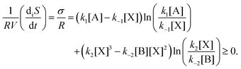
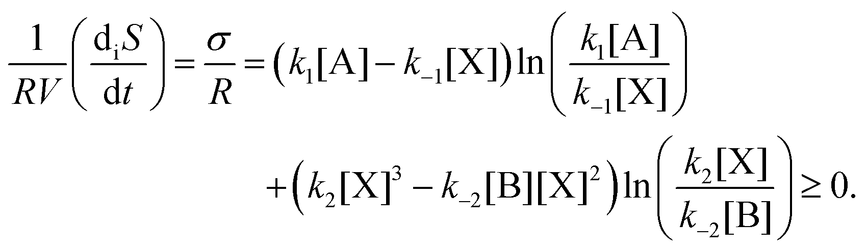
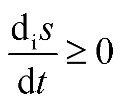
Chemical networks in far-from-equilibrium scenarios are conditioned by boundary conditions, and are paradigms of how systems function and evolve following the dictates as set down by non-equilibrium thermodynamics. In particular, the entropy production, that is, the rate of dissipation, the entropy exchanged between a system and its environment, and the overall balance of entropy are fundamental concepts in the thermodynamic characterization of far-from-equilibrium open systems, because they take into account the irreversibility of natural phenomena, as exemplified by (bio)chemical reactions, and by the functioning of biological cells. Moreover, a general inequality for the evolution of the entropy production, valid for the entire range of macroscopic physics and for fixed boundary conditions, was established by Glansdorff and Prigogine.20 This general evolution criterion (GEC), actually a theorem, has been extended recently to encompass well-mixed open-flow reaction systems.21 The new result is an inequality constraining the time rate of change of the entropy balance: the sum of the entropy production and the exchange entropy, or entropy flux, eqn (1), in open-flow chemical reacting systems. The fundamental importance of this extended inequality is that it governs the joint evolution of the reactions occurring within the system volume in conjunction with the input/output matter fluxes that couple the system with its environment (the boundary conditions). The GEC imposes a constraint on the way the chemical forces, or the affinities, can change in time. Its range of validity encompasses systems for which the assumption of local equilibrium holds (see Chapter II.2 of ref. 20 and Section 5 for further details).
The chemical Schlögl model has multiple steady states and represents a simple model for a first-order non-equilibrium phase transition.22,23 It has been widely used as a simple minimal model of bistability and bifurcation and for which thermodynamic analysis has been developed, for both deterministic and stochastic settings,24 see the review in ref. 25. The model was originally defined and analyzed under the assumption of a single time dependent species and two clamped or chemostated species. This clamped species approximation model continues to be used as a simple model of bistability to the present day. The approximation was most likely motivated for the purposes of mathematical convenience, but it is unrealistic from the entropic point of view. Indeed, it is known that non-equilibrium thermodynamics is founded on the balance equation for entropy:20
where
S is the total entropy, d
iS ≥ 0 is the entropy production, and d
eS is the entropy exchange (entropy flow) with the environment outside the system. For the original clamped Schlögl model, there is no entropy flow d
eS = 0, hence
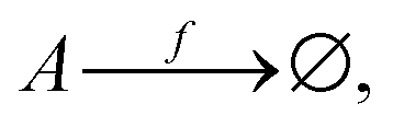
eqn (1) and (2) imply that the system's entropy increases asymptotically without limit, d
S/d
t > 0, and even for stationary states in the composition (concentration). When an entropy flux is established, say by a hydrodynamic flow of matter, then d
eS = −d
iS < 0 holds for all the possible stationary states;
26 the entropy flux cancels and compensates, or balances, the internal positive entropy production, and hence d
S/d
t = 0 on these states, so the system entropy
S remains constant. Nowadays, there are no valid arguments for continuing to use approximations which exclude the matter and energy exchange with the surroundings.
27–29
In this paper, our aim is to provide an entropic analysis of the Schlögl model, subject to open-flow and with a critical comparison to the clamped version. We place an important emphasis on the entropic exchanges and explore the specific non-equilibrium thermodynamic conditions under which bifurcation and bistability take place. We begin with a survey of the clamped model, bifurcation, and evaluate the entropy production on the non-equilibrium stationary states (NESS). We calculate the entropy production, showing how fluctuations about the unstable branch of NESS will lead either to the stable NESS of higher, or else lower, entropy productions, depending only on the sign of the concentration fluctuation about the unstable NESS. The general evolution criterion is validated in both cases, and we indicate how the GEC distinguishes qualitatively between the alternative transitions between unstable and stable states. We evaluate the kinetic potential associated with the change of the entropy balance with respect to the temporal derivative of the chemical forces (the affinities) which provides information regarding the relative stability of the stable NESS in the clamped version.
We next define and analyze a volumetric open-flow version of the Schlögl model, for which all three species evolve in concert dynamically, and calculate the entropy production and the exchange entropy thus confirming the compensation deS = −diS < 0 of the positive entropy production by the (negative) entropy flux for all NESS. The open-flow system possesses NESS that are absent in the clamped model, indicating that the dynamics of all three species is sensitive to how the system is maintained out of equilibrium. The open flow models considered here are bistable. Small concentration perturbations about the unstable NESS will lead either to the stable NESS of either higher, or else of lower, entropy productions, depending only on the sign of the compositional fluctuation about the unstable NESS, and we validate the generalization of the GEC for these fluctuations. The GEC distinguishes between these alternative transitions to stable states. In contrast to the one-dimensional clamped model, a global kinetic potential for these three-dimensional open flow models does not exist, since the corresponding differentials that would define the putative potential, are not exact.
Stoichiometric proportions reveal the topological structure of reaction networks, and their properties may be regarded as structural invariants. Important conclusions can be derived from stoichiometry, which complement the kinetic properties of the reaction network. We use stoichiometric network analysis (SNA)30 to obtain the so-called extreme flux modes (EFMs) corresponding to both the clamped and the open-flow models. These flux modes constitute the irreducible set of reaction pathways of the system. We evaluate the (hybrid) combinations of the partial entropy productions and exchange entropies associated with each uni-directional EFM. These partial reaction path dissipations indicate how the overall entropy production and exchange entropy are distributed, or partitioned, over each irreducible reaction pathway. The sum of the partial dissipations and entropy exchanges over the full set of EFMs yields the complete entropy balance, eqn (1).
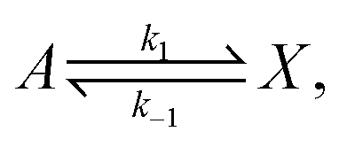
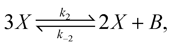
2 Schlögl: clamped
The original model22,23 is defined by the following reversible reactions:| |  | (3) |
| | 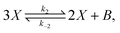 | (4) |
The concentrations [A] and [B] are held fixed (clamped), thus describing a scenario of infinite volume and static homogeneous concentrations in A and B, so that the only kinetic rate equation is that for the intermediate species [X], and is| | 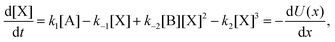 | (5) |
where U(x), with x = [X], defines the kinetic potential (see below). The NESS are plotted in Fig. 1 showing the bifurcation from the region of unstable NESS, delimited by the pair of red dots, to one of the two stable (upper or lower) regions of NESS. The external clamped concentration [B] serves as a measure from equilibrium, and the family of all stationary states continuously connected to equilibrium defines the thermodynamic branch.26 The set of all the stable and unstable NESS, belong to this thermodynamic branch, which is many-valued, Fig. 1. When the system becomes unstable, it makes a transition to one of the two stable regions of this branch (see below).
 |
| | Fig. 1 Thermodynamic branch. The bifurcation of non-equilibrium steady states [X]* as a function of the external clamped concentration [B]. Parameters: [A] = 1, k1 = 0.5, k−1 = 3, k2 = k−2 = 1. The lower and upper portions of the curve correspond to the stable NESS, the middle segment (delimited by red dots) to the unstable NESS. Compare to the graph of the kinetic potential in Fig. 3, calculated for [B] = 4. The equilibrium point is at  , see eqn (26). , see eqn (26). | |
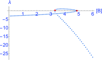
The local stability of the NESS is indicated by the sign and value of the eigenvalue λ, obtained by expanding the right hand side of eqn (5) about the stationary solutions [X]*, see Fig. 2:
| | | λ = −k−1 + 2k−2[B][X]* − 3k2[X]*2. | (6) |
This is evaluated in
Fig. 2 for all the individual NESS displayed in
Fig. 1, confirming the instability of the middle segment, that is, the hysteresis loop for which
λ > 0. Positivity implies any small fluctuation
δ[X](
t) about the stationary state [X]* will grow exponentially. In contrast, both the lower and upper portions of the thermodynamic branch, respectively, have
λ < 0, so here the fluctuations in concentration decrease with time exponentially returning the system to the initial stationary state [X]*. Note that the absolute values of
λ < 0 do not provide information about the relative stability of the two stable NESS. For this, the kinetic potential, when it exists, is required.
 |
| | Fig. 2 The eigenvalue λ, eqn (6), as a function of the external clamped concentration [B]. The interval of positive values λ > 0, delimited by the pair of red dots, corresponds to the unstable middle segment of the hysteresis loop in Fig. 1. The eigenvalues corresponding to the upper segment of stable NESS in Fig. 1 are more negative than those of the lower segment of stable NESS, implying that the associated potential well in Fig. 3, is locally more attractive than the other well. Parameters are as for Fig. 1. | |
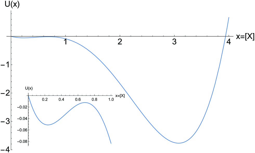
The function U appearing in eqn (5) defines an effective global kinetic potential, where we define a = [A], x = [X], b = [B]:
| |  | (7) |
(see
Fig. 3). The points in
U with vanishing derivative

correspond to the NESS. The other regions indicate the rate of change of the concentration [X]. In the region of bistability, for approximately 3.5 ≤ [B] ≤ 4.8, inspection of
Fig. 3 shows that the NESS corresponding to the absolute minimum are the more stable of the two. The NESS of the upper portion in
Fig. 1 are more stable than the NESS of the lower portion. Moreover, a relatively small fluctuation in concentration
δ[X] > 0 will take the system out of the stable NESS corresponding to the shallow relative minimum in
U(
x) into the lower absolute minimum. A very large concentration fluctuation would be required to overcome the now large potential barrier, in order to knock the system out of this absolute minimum.
 |
| | Fig. 3 The kinetic potential U(x), eqn (7). For [B] = 4, and the other parameters as in Fig. 1. The deep absolute minimum corresponds to the upper segment of stable NESS for large [X]. Inset: The region of small 0 < [X] ≤ 1 showing the relative minimum and the relative maximum, corresponding to the stable NESS on the lower segment, and the unstable NESS on the hysteresis loop, respectively. Compare to the two stable NESS and the one unstable NESS in Fig. 1 located at [B] = 4. | |
The entropy production per unit volume V is (R is the gas constant):
| |  | (8) |
This is plotted in
Fig. 4, for all the NESS calculated in
Fig. 1. This indicates that there is a bifurcation in the region of bistability 3.5 ≤ [B] ≤ 4.8 in the entropy production: the production is either less than or greater than that corresponding to the unstable segment of NESS, and which of these two outcomes depends only on the sign (±) of the compositional fluctuation about the unstable NESS: [X]* ±
δ[X]. From inspection of
U(
x), the NESS in the bistable region, having the greater entropy production are the more stable. Note there is no exchange entropy in the clamped model: d
eS = 0 (see Section 3).
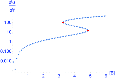 |
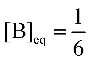
| | Fig. 4 Thermodynamic branch. The bifurcation in the entropy production eqn (8), where  , for the clamped model. Units are (J K−1 s−1 L−1). Parameters: [A] = 1, k1 = 0.5, k−1 = 3, k2 = k−2 = 1. The lower and upper segments correspond to stable NESS, the middle segment (delimited by the pair of red dots) corresponds to the unstable NESS. The entropy production goes to zero at [B] = 1/6 corresponding to the equilibrium state of the system. , for the clamped model. Units are (J K−1 s−1 L−1). Parameters: [A] = 1, k1 = 0.5, k−1 = 3, k2 = k−2 = 1. The lower and upper segments correspond to stable NESS, the middle segment (delimited by the pair of red dots) corresponds to the unstable NESS. The entropy production goes to zero at [B] = 1/6 corresponding to the equilibrium state of the system. | |
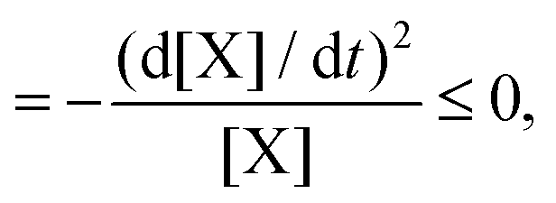
For macroscopic physics with fixed boundary conditions, the general evolution criterion (GEC),20 states that the change of the so-called generalized forces proceeds always in a way as to lower the value of the entropy production. In the case of chemical reactions, these forces are the chemical affinities. For the above reaction model, the GEC is (dA/dt stands for the change due to temporal derivatives of the affinities A)
| |  | (9) |
| |  | (10) |
and is zero on any NESS. The second line follows by using the rate equation
eqn (5), and so renders the inequality of the GEC manifest. We evaluate this expression in
Fig. 5 using
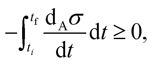
eqn (9) for the transition from an unstable NESS to first one, and then to the other, of the two stable NESS's. As predicted by the GEC, this quantity vanishes on the NESS, and is strictly negative definite along the dynamic transition from one NESS to another. Note that the GEC holds for the transition from an unstable NESS to either one of the two stable NESS's. However, the integrated dissipation, due to the changes in the chemical affinities along each individual transition (minus the integral over the transition time),
| |  | (11) |
is not the same: see
Fig. 5. This follows since the integrated dissipation increases with the distance (in the concentration [X]*) from the unstable to the stable NESS. This distance decreases for transitions from the unstable to the stable NESS on the lower portion, but increases for transitions to the stable NESS on the upper portion, respectively, as [B] increases in the range 3.3 ≤ [B] ≤ 4.9, see
Fig. 1.
 |
| | Fig. 5 Validation of the GEC eqn (9) at [B] = 4. (A) Starting from the unstable NESS with a small negative compositional fluctuation δ[X] < 0 initiates the evolution of the system toward the lower stable NESS (see Fig. 1). (B) A small positive compositional fluctuation δ[X] > 0 initiates the evolution of the system toward the higher stable NESS (see Fig. 1). The quantity  is zero at both the initial and final NESS, and is manifestly negative during the transition from the unstable to the stable NESS. The units are (J K−1 s−2 L−1). The integrated dissipations are distinct for each transition, as quantified by (minus) the integrals over the transition times eqn (11). The behavior depicted here is qualitatively similar if we start the system off from any one of the unstable NESS in Fig. 1 for increasing [B] > 3.3: the (absolute value of the) time-integrated dissipation for the transit to the upper segment of stable NESS is greater (right) than that for the transit to the lower segment of stable NESS (left). is zero at both the initial and final NESS, and is manifestly negative during the transition from the unstable to the stable NESS. The units are (J K−1 s−2 L−1). The integrated dissipations are distinct for each transition, as quantified by (minus) the integrals over the transition times eqn (11). The behavior depicted here is qualitatively similar if we start the system off from any one of the unstable NESS in Fig. 1 for increasing [B] > 3.3: the (absolute value of the) time-integrated dissipation for the transit to the upper segment of stable NESS is greater (right) than that for the transit to the lower segment of stable NESS (left). | |
2.1 Kinetic potential for GEC
For a single variable, a global kinetic potential Φ exists such that TdXσ = dΦ ≤ 0, and can be calculated straightforwardly.20 Following that development, we find that| |  | (12) |
Then the potential is| |  | (13) |
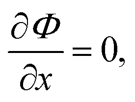
where α is a constant and we write a = [A], x = [X], b = [B]. Note that in a steady state, the potential has extremum at| |  | (14) |
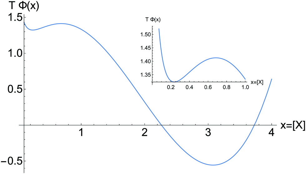
As it follows immediately from eqn (12) or eqn (13). This extrema (NESS) can be appreciated in the graph of Φ plotted in Fig. 6. The stability conditions for these stationary states implies20| |  | (15) |
which holds for both the relative minimum and the absolute minimum in Fig. 6. The extrema coincide with those for U(x), and TΦ indicates that the more stable of the two stable NESS corresponds to the stationary states located on the upper region of Fig. 1. If we imagine the system is initially at the unstable NESS, located at the relative maximum in Fig. 6, then a small negative concentration fluctuation will tip the system to the left and toward the relative minimum. The distance down the potential well is approximately TΔΦ = 0.10 (in arbitrary units), whereas a small positive fluctuation tips the system to the right, toward the absolute minimum, and the distance down the well is greater: TΔΦ = 1.92. Thus the greater dissipation is along this latter transition, as reflected in Fig. 5.
 |
| | Fig. 6 The global kinetic potential for the GEC eqn (13) evaluated at [B] = 4 and scaled by the temperature T and for α = 0. Note the positions of the relative minimum and maximum and the absolute minimum in the stationary composition x = [X]. Inset: The region 0 < x ≤ 1. The absolute minimum is that reached by the system in a transition from the unstable NESS (the relative maximum) leading to the larger integrated dissipation due to changes in the affinity. Compare and contrast to Fig. 5 and 4. | |
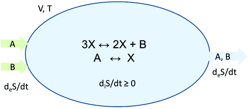
3 Schlögl: open flow
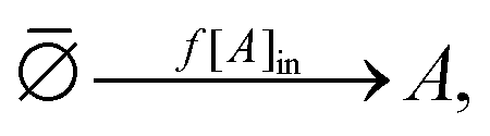
In keeping with the specification of the original clamped model, Section 2, and to facilitate comparisons, we maintain X within the reactor volume V, and allow input and output volumetric flow terms for both the A and B species (see Fig. 7), where ∅ represents the environment external to the reactor:| |  | (16) |
| |  | (17) |
| |  | (18) |
| |  | (19) |
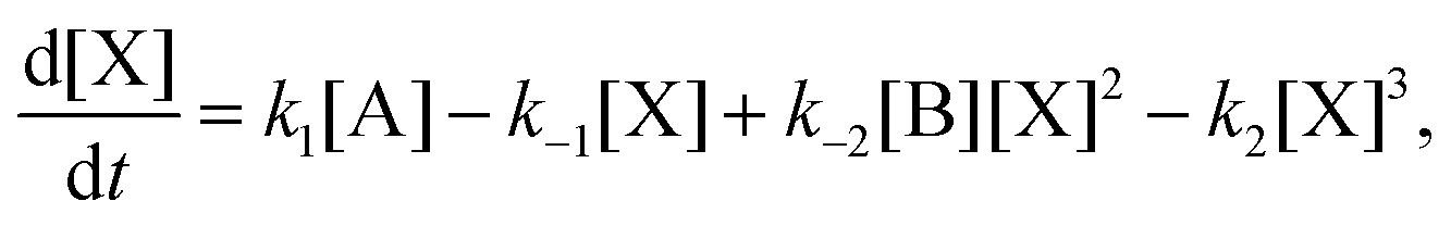
[A]in and [B]in are the input concentrations, and f = q/V, with q in units of L s−1, is the volumetric flow rate. In this case, there are now three coupled differential rate equations:| |  | (20) |
| |  | (21) |
| |  | (22) |
 |
| | Fig. 7 Open-flow version of the Schlögl model in a well-stirred isothermal reaction tank of volume V. Species A and B flow in at fixed concentrations [A]in and [B]in, respectively, and both flow out (represented by the pseudo-reactions eqn (16)–(19)) with their instantaneous concentrations as determined by the rate equations, eqn (20)–(22). X remains in the reactor, as in the original clamped version, see Section 2. The volumetric flow terms give rise to the exchange entropy per unit volume,  , which is required for achieving entropy balance at any NESS: , which is required for achieving entropy balance at any NESS:  , see eqn (1). , see eqn (1). | |
The stationary solutions are plotted in Fig. 8. In marked contrast to the clamped model in Section 2, all three species A, X, and B actively participate in the bifurcation. The input concentration [B]in provides a measure of the distance from equilibrium; and this is given by [B]in − [B]eq, where [B]eq is calculated from eqn (26). The input rate of fluid flow is fixed and equal to the outflow rate. This boundary condition takes the internal reaction network away from equilibrium as [B]in increases beyond [B]eq, thus increasing the chemical forces (the affinities)  and
and  acting on the internal reaction network. The system is then near (far from) equilibrium when
  .
.
 |
| | Fig. 8 Thermodynamic branches. The bifurcations of non-equilibrium steady states (a) [X]*, (b) [A]*, and (c) [B]*, as functions of the input concentration [B]in. Parameters: [A]in = 10−2, k1 = 2, k−1 = 30, k2 = k−2 = 10, f = 10−3. The lower and upper parts of each thermodynamic branch of steady states for each concentration correspond to stable NESS, while the middle segments (delimited by the pair of red dots) correspond to the unstable NESS. The thermodynamic branch for [B]* in (c) is inverted (“turned over”) with respect to the branches of [A]* in (b) and [X]* in (a), while the latter two are qualitatively similar to each other, differing only by overall scale. | |
The family of all steady states continuously connected to equilibrium defines the thermodynamic branch.26 There is a thermodynamic branch for each species. The thermodynamic branches are many-valued, so that the system can suffer a bifurcation from an unstable region of a branch to a different stable region, of the same branch. Whereas the branches of the set of NESS for A and X are qualitatively similar to each other and to that of X in the clamped model, and that of B is inverted or “turned-over” with respect to those of A and X, see Fig. 8. This implies that the concentrations [A], and [X] will both either increase or decrease in tandem, whereas the concentration of [B] will evolve always in the opposite sense to A and X during a transition from an unstable to a stable NESS. Note the overall net reaction in eqn (3) and (4) is A ⇌ B and so “un-clamping” the externally supplied species allows for the alternance, or switching, in the relative magnitudes of their steady state concentrations within the bistable regime. This “see-saw” phenomena in [A], and [B] is entirely absent in the clamped model. See also the entropic analysis of the associated extreme flux modes in Section 4.
The local stability of the NESS is determined from the eigenvalues of the 3 × 3 Jacobian associated with the kinetic equations eqn (20)–(22):
| |  | (23) |
where [B]*, [X]* denote the concentration values at the NESS (see
Fig. 8). The three eigenvalues
λ1,
λ2, and
λ3 are calculated for each NESS, for a range of input concentrations [B]
in, as displayed in
Fig. 9. The eigenvalue
λ3 is positive on the hysteresis loop of the NESS, indicating its instability. All three eigenvalues are strictly negative on all the other NESS, indicating their local stability.
 |
| | Fig. 9 The three eigenvalues of the Jacobian eqn (23) calculated as functions of the input value [B]in, the other parameters are the same as for Fig. 8. Since (a) λ1 < 0 and (b) λ2 < 0 are negative, the region of instability is tracked solely by (c) λ3 > 0, and its domain of positivity corresponds to the NESS on the middle segments (bounded by the red dots) of the thermodynamic branches in Fig. 8. | |
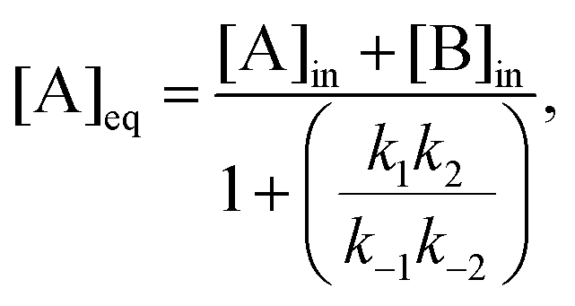
The entropy production per unit volume V is given in eqn (8), and the exchange entropy per unit volume, due to the volumetric open flow eqn (16)–(19), is27
| |  | (24) |
where the equilibrium concentrations are given by
| |  | (25) |
| |  | (26) |
| |  | (27) |
These are the values of the concentrations the system would relax to (detailed balance) if the reactor were to be isolated, or the fluid flow suddenly shut off (
f = 0) after the system is allowed to reach a NESS, see
Fig. 7. These equilibrium values correspond to the total chemical mass of the system, determined by the input concentrations [A]
in, [B]
in of the open system, as well as by the reaction rate constants. Due to entropy balance
eqn (1), the exchange entropy
eqn (24) will be negative
σe < 0 on all the NESS, see
Fig. 10 where entropy production and exchange entropy are calculated. The exchange entropy, calculated independently, using
eqn (24), mirrors the behavior of
σ with respect to the abscissa: see
Fig. 10.
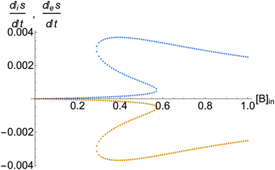 |
| | Fig. 10 The upper curve: the entropy production per unit volume:  , eqn (8). The lower curve: the exchange entropy per unit volume: , eqn (8). The lower curve: the exchange entropy per unit volume:  eqn (24), evaluated at the NESS as functions of the input concentration [B]in. System entropy is balanced on all the NESS: eqn (24), evaluated at the NESS as functions of the input concentration [B]in. System entropy is balanced on all the NESS:  , see eqn (1). Units are (J K−1 s−1 L−1). Compare to Fig. 4, for the clamped model, for which there is no exchange entropy. , see eqn (1). Units are (J K−1 s−1 L−1). Compare to Fig. 4, for the clamped model, for which there is no exchange entropy. | |
The statement of the general evolution criterion (GEC)21 corresponding to this open-flow model is as follows:
| |  | (28) |
and is strictly zero at any NESS. This result follows from adding the expressions for the entropy production
eqn (8) and exchange entropy
eqn (24) and differentiating the forces (the chemical affinities) with respect to time. Using the rate equations
eqn (20)–(22) allows us to cast the results of that calculation back in terms of the rate equations and concentrations, resulting in the manifestly negative definite quadratic form.
We validate the GEC in Fig. 11, which shows the calculation of  for the transition, at [B]in = 0.4, from the unstable NESS to the stable NESS on the upper portion of the bifurcation curves for A and X (and lower portion of the B-bifurcation curve) (see also Fig. 8). Fig. 12 shows the dynamics and the GEC for the transition to the other stable NESS located on the lower portion of the bifurcation curves for A and X (and on the higher portion of the B-bifurcation curve). The behavior of the transitions from the segment of the unstable NESS to either one of the two alternative stable NESS's, is qualitatively similar to the results displayed here. A positive fluctuation in concentration added to either A or to X, or a negative fluctuation in concentration added to B leads to results qualitatively similar to those in Fig. 11. On the other hand, a negative fluctuation added to either A or to X, or a positive fluctuation added to B leads to results qualitatively similar to those in Fig. 12. We have validated the GEC for all these cases. The GEC is obeyed for all the transitions between unstable and stable NESS.
 |
| | Fig. 11 (a) Dynamic transition from the unstable NESS to the stable NESS located at [B]in = 0.4, when a small positive fluctuation δ[A] > 0 is added to [A]* (see Fig. 8(a)). Concentrations [A] and [X] both increase in tandem to reach their respective higher stable values, while [B] decreases to its lower stable value; compare to Fig. 8. (b) Validation of the GEC for this transition; the units are (J K−1 s−2 L−1). | |
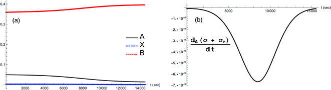 |
| | Fig. 12 (a) Dynamic transition from the unstable NESS to the stable NESS located at [B]in = 0.4, when a small negative fluctuation δ[A] < 0 is added to [A]* (see Fig. 8(a)). Concentrations [A] and [X] both decrease in tandem to reach their respective lower stable values, while [B] increases to its higher stable value; compare to Fig. 8. (b) Validation of the GEC for this transition; the units are (J K−1 s−2 L−1). | |
Finally, an attempt to define and calculate a kinetic potential for the coupled reaction rate equations (eqn (20)–(22)) fails because we can prove that the differential form,
| | | dΦ = Fa(a, x, b)da + Fx(a, x, b)dx + Fb(a, x, b)db, | (29) |
where
Φ stands for the putative potential and the functions
Fa,
Fx, and
Fb are given by the right-hand sides of the rate equations
eqn (20)–(22), respectively, is not exact (see the ESI
†). By the same token, there is no global kinetic potential for the GEC,
i.e., for

. Conditions for the existence of a local potential however are given in Chapter IX of
ref. 20, but even the existence of a local potential beyond the linear regime is not guaranteed.
4 Dissipation and entropy exchange along elementary flux modes
Additional insight for describing reaction networks is provided by stoichiometric network analysis (SNA).30–34 The description in terms of the so-called elementary flux modes (EFM), or extreme currents (the irreducible set of linear combinations of the one-way rate velocities) is built up from both the chemical reactions and the volumetric matter flows. The EFMs reveal the explicit mechanisms of dissipation and of entropy exchange in a given network. SNA is based on stoichiometry, involves the system as a whole, and treats both the one-way reactions and flow terms on an equal footing.
The differential kinetic rate equations corresponding to the set of reactions and flows in eqn (20)–(22) can be written in compact matrix form, where x denotes the vector of concentrations, ν is the stoichiometric matrix and v is the vector of reaction rates (including the pseudoreactions corresponding to input output matter flows):
| |  | (30) |
The chemical pathway structure is an invariant property of the reaction network.
30 This pathway structure follows from the steady state condition
0 =
νv, which defines the right null space of
ν, and corresponds to the set of all stationary solutions
v of
eqn (30). Since the reaction rates are positive-definite
vj ≥ 0, ∀
j, these stationary solutions must belong to the intersection of this null space with the positive orthant
Rr+. This intersection defines a convex polyhedral cone
Cv spanned by a set of
M minimal generating vectors or elementary flux modes (EFM)
Ei's:
| |  | (31) |
These vectors {
Ei}
Mi=1 have
r-components, equal to the number of unidirectional reactions (including the flow terms)
30 and point along the
M edges of the cone
Cv. The
Ei correspond to subsets, or combinations, of several of the unidirectional reactions in
eqn (3), (4) and (16)–(19). Some of these EFMs may involve the coupling of the pseudoreaction fluxes with the chemical transformations, and may not necessarily include simultaneously both the forward and reverse steps of a specific chemical reaction.
The partitioning, or distribution, of the entropy production and entropy exchange over these EFMs gives a unique way to see how the coupling between reactions and matter currents determines the physical and chemical behavior of the complete network. Below we deduce the EFMs corresponding to the clamped and the open-flow versions of the Schlögl model, calculate the partial (and generally hybrid) entropy productions and exchanges along each EFM on the NESS. We analyze and contrast the results between these models. For further details regarding the methodology and applications of SNA, see ref. 21, 27 and 34.
4.1 Clamped model
According to SNA, the clamped model has the two extreme flux modes (EFMs):| | | E1 = 3X → 2X + B, B + 2X → 3X | (32) |
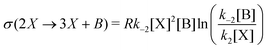
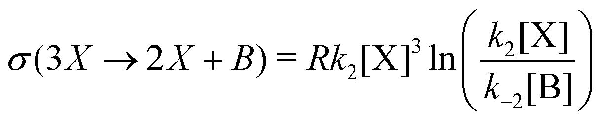
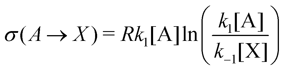
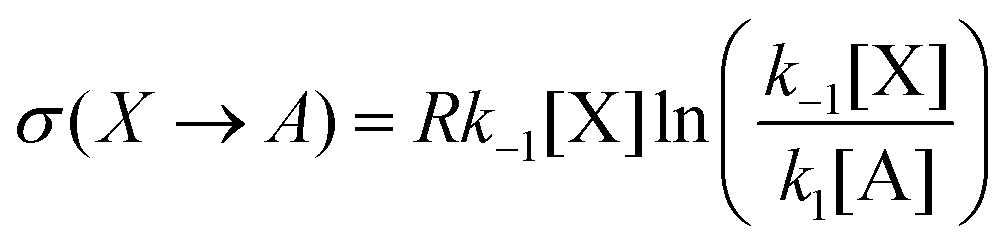
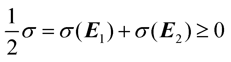
In this case, the forward and reverse transformations of each of the two reversible reactions, eqn (3) and (4), defines an EFM. Then from Table 1, we can calculate the amount of entropy production along each individual EFM:| | | σ(E1) = σ(3X → 2X + B) + σ(B + 2X → 3X) ≥ 0, | (34) |
| | | σ(E2) = σ(A → X) + σ(X → A) ≥ 0, | (35) |
and give the sought-after decomposition of the overall entropy production (per unit volume) σ = σ(E1) + σ(E2), see eqn (8). The overall net entropy production is distributed over each EFM as indicated in Fig. 13. For NESS up the first turning point, the greater relative dissipation is along E1 with respect to E2. It continues to increase along each EFM for the hysteresis loop of unstable NESS. Beyond the second turning point, it subsequently decreases for E1 while increasing monotonically for E2. The sum of the entropy production along both EFMs yields Fig. 4. There is no exchange entropy σe = 0.
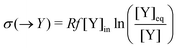
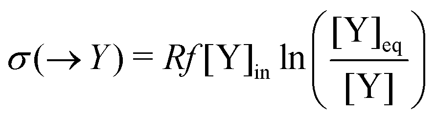
Table 1 The one-way transformations involved in the Schlögl model, eqn (3) and (4), and the corresponding one-way partial entropy “productions” and the entropy exchanges (per unit volume); R is the gas constant. Y may stand for A, X or B, respectively, depending on the input/output flow configuration, eqn (16)–(19), of the model. [Y]eq is the equilibrium concentration that [Y] would relax to if the flow were shut-off: f = 0, after the system reaches a NESS, see eqn (25)–(27)
| Transformation |
Partial entropy production or exchange |

|

|

|
|

|

|

|

|

|
|

|

|
 |
| | Fig. 13 Partitioning of the entropy production along the two elementary flux modes of the clamped Schlögl model, Section 2. (a) σ(E1), eqn (34) and (b) σ(E2), eqn (35). The sum of these two contributions yields the total entropy production, see eqn (8) and Fig. 4. The region of unstable NESS and bistability is bounded by the pair of red dots. Units are (J K−1 s−1 L−1). | |
4.2 Open flow
From SNA, the open flow version, Fig. 7, has the following six extreme flux modes (EFMs), each one made up from a particular subset of one-way reactions and flow terms as follows:| | | E1 = 3X → 2X + B, B + 2X → 3X | (36) |
| | | E5 = →B, B + 2X → 3X, X → A, A→ | (40) |
| | | E6 = →A, A → X, 3X → 2X + B, B→ | (41) |
E1 and E2 correspond to the two reversible reactions, eqn (4) and (3), whereas E3 and E4 represent the unreactive flow-through from the input to the output of B and A, respectively; see eqn (16)–(19). The EFM E5 represents the sequence of the two reverse reactions driven by the input of B and the output of A. The EFM E6 represents the sequence of the two forward reactions in eqn (3) and (4) driven by the input of A and the output of B. The overall pathways E5 and E6 are traversed in opposite flow directions: either from B to A, or else from A to B, and both these open pathways are productive. The opening of the Schlögl model to such volumetric matter flows creates the four additional EFMs that are absent from the clamped version.
The partial entropy productions and exchanges associated with each EFM, or pathway, are defined as follows:
| |  | (42) |
| |  | (43) |
| |  | (44) |
| |  | (45) |
| |  | (46) |
| | 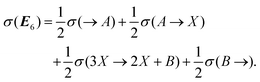 | (47) |
The coefficient factors of one-half are due to the fact that each one-way chemical transformation and flow term in
eqn (36)–(41) appears in two distinct EFMs. The expressions on the right hand side are evaluated explicitly with the help of
Table 1. We note that the entropy production

and exchange entropy

. In contrast to the clamped model, exactly half of the entropy production is distributed over the first two EFMs. And half of the exchange entropy, void in the clamped model, is distributed over the second pair of EFMs; see
Fig. 14. The other halves

are distributed over the final two EFMs, and in a hybrid, or composite, way; as concatenations of one way entropy “productions” and one-way exchange entropies, see
Fig. 15.
 |
| | Fig. 14 Open-flow model. The partial entropy productions (a) σ(E1) ≥ 0 and (b) σ(E2) ≥ 0 and the partial exchange entropies (c) σ(E3) ≤ 0 and (d): σ(E4) ≤ 0 evaluated on the NESS, versus the input concentration [B]in. For each curve, the region of unstable NESS and bistability is enclosed by the pair of red dots. These four contributions, two entropy productions plus two exchange entropies, sum to zero on the NESS: see eqn (48) when  . Units are (J K−1 s−1 L−1). . Units are (J K−1 s−1 L−1). | |
 |
| | Fig. 15 Open-flow model. The hybrid one-way entropy “productions” and exchange entropies. Top curve: σ(E6) and bottom curve: σ(E5). These satisfy σ(E5) = −σ(E6) on the NESS: eqn (48) when  . The region of unstable NESS bistability and switching is indicated for σ(E6) (σ(E5)) by the pair of red (black) dots. Units are (J K−1 s−1 L−1). . The region of unstable NESS bistability and switching is indicated for σ(E6) (σ(E5)) by the pair of red (black) dots. Units are (J K−1 s−1 L−1). | |
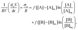
The entropy balance equation eqn (1), where s = S/V is the entropy per unit volume, can be written in terms of the EFMs as follows:
| |  | (48) |
Hence for all NESS we have

and
σ(
E5) = −
σ(
E6). The latter two EFMs can undergo a mutual switching in their relative ± signs when the system is in an unstable NESS. A compositional fluctuation about the unstable region in
σ(
E6) (or about the mirror image point in
σ(
E5)) can provoke a transition to either a greater positive or to a lesser negative value in
σ(
E6) and correspondingly, to a more negative value or a greater positive value in
σ(
E5). The latter case gives rise to the switching in signs. The entropy balance is maintained, see
Fig. 15. These EFMs
E5 and
E6 are related by time-reversal. The time-reversal operation flips the direction of the reaction and flow arrows, interchanging forward and reverse transformations, we see that
E5 and
E6 form a time-reverse pair of pathways. The first four EFMs are then singlets under time-reversal: they transform into themselves under this operation. Note the contrast with models of SMSB whose EFMs can be classified as being either parity (enantiomeric) singlets or doublets.
21
Other possibilities for implementing volumetric open-flow, include, for example, having only A or B flow in to the reactor, while allowing for all three species A, X, and B to flow out with their instantaneous concentrations. In the former case, when only A flows in, there is no regime of bistability, but there is in the latter case, when only B flows in. For both scenarios, there are now five EFMs, instead of six, and the difference between either the A or the B input flow arrangement is readily appreciated in the structure of these five extreme flux modes, as well as in the forward or reverse directions the chemical transformations in the reactor are driven by these flows; see the ESI.†
5 Conclusions
We may summarize our main results in the following points:
(1) Clamped versus open flow. Connecting the reacting system to volumetric flows leads to important dynamic and thermodynamic differences with the clamped model. On the one hand, all three species A, X and B participate fully in the dynamics of the bistability, as manifested in the overall reaction A ⇌ B, which is suppressed when the external concentrations are held fixed. Secondly, the flows allow for entropy exchange with the environment, and these entropy fluxes together with the entropy production, obey the entropy balance equation eqn (1). The entropy production is now exactly compensated by the entropy exchange on all the stationary states, implying that the system entropy remains constant on all these states.
Further information distinguishing the clamped from the open-flow versions is provided by the EFMs, as determined by SNA. We have shown how these flux modes indicate the way in which both the entropy production and the exchange entropy are distributed, or partitioned, over the complete reaction network, including the flows. We distinguish three types of EFMs: (i) closed pathways, which can be described as micro-reversible transformations, made up from the pair of forward and reverse one-way reactions, (ii) open un-reactive pathways formed by the input and output flows, which involve no reactions per se and, (iii) open pathways which are hybrid concatenations of strictly one-way chemical reactions plus one-way input and output flows, which are at the heart of the irreversibility of the system. The latter two types are absent from the clamped model. The significance of type (ii) is that they impose the constraint of the boundary condition on the entropy balance eqn (1). For type (iii) pathways, there is an overall unidirectional flow of matter which begins at the input, passes through a specific sequence of one-way reactions for type (ii), and then exits from the output to the environment. These describe the thermodynamic irreversibility of the system, and are absent from the clamped model. For the closed EFMs of type (i), the associated fraction of the overall entropy production is always positive and there is no exchange entropy. By contrast, for the open EFMs, the weighted hybrid sum of the corresponding one-way entropy “productions” and one-way exchange entropies can be either positive or negative. For type (ii), the sum over one-way entropy exchanges yields the overall entropy exchange for that EFM, which can be either positive or negative. We have seen moreover, in the open flow model, that this algebraic sign can switch in the bistable regime between a specific pair of hybrid type (iii) EFMs. Most importantly, the sum of all the one-way entropy productions and entropy exchanges over the complete set of EFMs yields the entropy balance equation, eqn (1), and hence this sum over the extreme flux modes is strictly zero for all NESS.21,27,28,35
(2) General evolution criterion (GEC). This is a general inequality valid for the evolution of a macroscopic system under fixed boundary conditions.20 Recall that the entropy production per unit volume can be expressed as the sum over products of the generalized forces Fi times the currents Ji:26
| |  | (49) |
The GEC states that the generalized forces (the affinities in the case of chemical reactions) will change in time so as to lower the entropy production:
| |  | (50) |
with equality to zero holding at a NESS. However, this result by itself does not imply that the entropy production will actually be lowered or even minimized, since the GEC does not involve a total derivative in the time. Indeed, apart from the evolution of the generalized forces
Fi, there is a second contribution to the total time derivative of the entropy production d
σ/d
t which involves the change in time of the currents
Ji, and this contribution d
Jσ/d
t can be either positive or negative in the non-linear regime of non-equilibrium thermodynamics. In macroscopic physical and chemical systems, the GEC is the only established theorem (it is not a “principle”) governing the evolution of the entropy production (and the entropy exchange in well-mixed chemical systems) for non-equilibrium thermodynamics. It is only in the restricted linear regime of non-equilibrium thermodynamics where the change with respect to the currents is linearly proportional to the change with respect to the forces, and then here and only here does the GEC reduce, as it must, to Prigogine's theorem of minimum entropy production.
26 But in the much more interesting and complicated non-linear regime, to date there is no rigorously proven maximum/minimum entropy production theorem (see below).
Eqn (10) is a special case of the general result derived for GEC for well-mixed reacting systems.21 The calculation, in passing from eqn (9) to eqn (10), demonstrates that dAσ/dt is manifestly semi-negative definite, and is strictly zero for stationary states. See also the expression of the GEC for the open-flow case which includes the exchange entropy. The manifestly semi-negative definite inequality again results automatically and manifestly, in accord with the general result obtained in ref. 21.
We have focused our attention on the limit of large volumes and large number of molecules: the thermodynamic limit, for which the reaction-rate equations work very well.36 For small enough systems, and for molecular populations not too many orders of magnitude larger than one, discreteness and stochasticity may play important roles.37 In this discrete and stochastic domain, an inequality reminiscent of the Glansdorff and Prigogine GEC, was established by Nicolis and coworkers38 and involves the probability distribution P(X, t) where X is the state vector:
| |  | (51) |
and A is the chemical affinity. The inequality is manifest, since
P(
X,
t) ≥ 0. The equality to zero holds for stationary configurations. Thus, the affinities (now stochastic variables) must evolve in time so as to lower the entropy production. Yet, just as for the deterministic case, this result by itself does not imply that the entropy production will actually be lowered or even reach a minimum, since there is a second contribution to the total time derivative of the entropy production due to the temporal change in the stochastic fluxes.
38 Again, it is only in the linear regime that the entropy production reaches a minimum value, as demonstrated for stochastic dynamics.
38 Note the formal correspondence between the deterministic and stochastic versions of the GEC, in which the deterministic concentrations are replaced by the probability distribution of the particle numbers:
and the sum over species is replaced by the sum over configurations; compare
eqn (9) and (28) to
eqn (51) and see also
ref. 21.
Some comments concerning the domain of validity of the GEC are warranted. The proof of the GEC appeals to the local equilibrium hypothesis, or assumption; see Section II.2 in ref. 20. This assumption is valid for complex systems of chemical reactions with highly nonlinear kinetics provided the rate of elastic collisions remains larger than the rate of reactive collisions. This includes the Schlögl model treated here. Convective and transport effects described by Navier–Stokes equations are also within the domain of validity of the local description. On the contrary, shock waves, and plastic deformations of solids lie outside the range of this local equilibrium approach. Clearly then, in these exceptional situations, where the local equilibrium hypothesis does not hold, we would a priori not expect the GEC to be valid.
The GEC in general gives no information concerning the putative stability of the non-equilibrium stationary states (NESS) in the non-linear regime of non-equilibrium thermodynamics. This is because the GEC cannot be related in general to a kinetic potential. On the other hand, it does govern the way the generalized forces evolve, and this force-evolution connection is the purpose of this paper. In the original proofs of the GEC, equilibrium stability conditions are carried over to non-equilibrium thermodynamics by appealing to the local equilibrium hypothesis. On the other hand, the stability question of the NESS is a major goal of studying the temporal dependence of the so-called excess entropy production, and its relation to Lyapunov functionals, a rather different problem than the topics treated here. In these stability investigations, the NESS need not arise from local equilibrium, as shown in ref. 39.
(3) Entropy production. For the model studied here, a compositional fluctuation about the unstable non-equilibrium stationary state in the bistable region can initiate the evolution of the system toward either the upper or lower regions of stable stationary states on the many-valued thermodynamic branch, and hence toward final states yielding either greater or lesser entropy productions with respect to the unstable states. This conclusion holds for both the clamped and volumetric open flow versions of the Schlögl model. Previous reports on the bistability and spontaneous mirror symmetry breaking in enantioselective catalysis show a qualitatively similar behavior but, when the thermodynamic branch becomes unstable, moreover, the increase or decrease in the change in the entropy production does not correlate with an increase or decrease of the affinities.35 We emphasize this because the only theorem21 concerning the temporal behavior of the entropy production (and the exchange entropy in open flow systems) is the general evolution criterion (GEC) eqn (28). Therefore, we find no evidence for the validity of an entropy maximization “principle”, such for example, as has been proposed in climate science40 and in physics.41 Careful refutations have already been made elsewhere arguing against such a principle,42,43 and we are in agreement with the counterexamples offered therein. The sole theorem concerning the temporal behavior of the entropy production in far-from-equilibrium situations is the general evolution criterion (GEC), and it holds in both deterministic and stochastic non-equilibrium thermodynamics. In far-from-equilibrium situations, a flow of energy may either increase the entropy production, by adding a new mechanism of dissipation, or it can decrease it, as in symmetry breaking instabilities.20 In the latter, some of the existing mechanisms of dissipation that are involved in maintaining the symmetry are suppressed, or greatly diminished in their productivity and reactivity, after the symmetry is broken. Thus, for example, mirror symmetry involves two subsets of enantiomerically related mechanisms of dissipation. After mirror symmetry breaking, the subset of reaction pathways involving the minority enantiomer becomes practically inoperative,21,28,29,35 and this lowers the overall entropy production.
Concerning the relevance of this work for actual chemical systems presenting bistable behavior, we may mention the replicator and catalytic networks giving rise to an array of emergent phenomena such as cooperation, chemical computation, bifurcation, and chemical oscillations, as reviewed in ref. 44. As emphasized there, the most interesting emergent phenomena leading to complexification and emergence requires open systems. In these latter cases, entropy will be continuously produced and exchanged with the environment. The general evolution criterion then dictates that the chemical forces will change in time so as to lower the dissipation during the system's approach to the (stable) non-equilibrium stationary state (NESS). For oscillations, there are no NESS's, so the rate of change of the dissipation with respect to the chemical affinities will be always negative and oscillating. This has been confirmed numerically for the chiral oscillations that result from the mirror symmetry breaking in chiral catalytic networks.45 A recent report on bistability in a thiodepsipeptide replicator network involves switching between a (high) NESS populated by coiled-coil peptides and a (low) NESS populated by unfolded precursors.46 Our work here indicates that the coiled peptide state will have the larger entropy production in the region of bistability. Moreover, since the model operates under clamped conditions, it may be possible to estimate a kinetic potential associated with the changes of the entropy production with respect to the affinities. Such a potential could then be used to study the relative stability of the two stationary states (coiled and unfolded) with respect to variations in the system parameters: rate constants, the (clamped) thiol concentration, the temperature, the denaturation factor, etc., and hence explore the bistability parameter space based on entropic principles alone, and to check against the experimental exploration of this parameter space.
Conflicts of interest
There are no conflicts to declare.
Acknowledgements
The authors acknowledge the coordinated research grants CTQ2017-87864-C2-1(2)-P (MINECO), Spain.
Notes and references
- J. E. Lisman, Proc. Natl. Acad. Sci. U. S. A., 1985, 82, 3055–3057 CrossRef CAS PubMed.
- A. W. Murray and M. W. Kirschner, Science, 2006, 246, 614–621 CrossRef PubMed.
- D. Gonze and A. Goldbeter, J. Theor. Biol., 2000, 210, 167–186 CrossRef PubMed.
- K. C. Chen, A. Csikasz-Nagy, B. Gyorffy, J. Val, B. Novak and J. J. Tyson, Mol. Biol. Cell, 2000, 11, 369–391 CrossRef CAS PubMed.
- F. R. Cross, V. Archambault, M. Miller and M. Klovstad, Mol. Biol. Cell, 2002, 13, 52–70 CrossRef CAS PubMed.
- W. Sha, J. Moore, K. Chen, A. D. Lassaletta, C.-S. Yi, J. J. Tyson and J. C. Sible, Proc. Natl. Acad. Sci. U. S. A., 2003, 100, 975–980 CrossRef CAS PubMed.
- A. R. Reynolds, C. Tescher, P. J. Verveer, O. Rocks and P. I. H. Bastiaens, Nat. Cell Biol., 2003, 5, 447–453 CrossRef CAS PubMed.
- W. Xiong and J. E. Ferrell, Nature, 2006, 426, 460–465 CrossRef PubMed.
- N. I. Markevich, J. B. Hoek and B. N. Kolodenko, J. Cell Biol., 2004, 164, 353–359 CrossRef CAS PubMed.
-
I. Epstein and J. Pojman, An Introduction to Nonlinear Chemical Dynamics: Oscillations, Waves, Patterns and Chaos, Oxford, New York, 1st edn, 1996 Search PubMed.
- G. Craciun, Y. Tang and M. Feinberg, Proc. Natl. Acad. Sci. U. S. A., 2006, 103, 8697–8702 CrossRef CAS PubMed.
- J. Kim, S. W. Kristin and E. Winfree, Mol. Syst. Biol., 2006, 2, 68 CrossRef PubMed.
- F. Muzika, T. Bansagi, I. Schreiber, L. Schreiberova and A. F. Taylor, Chem. Commun., 2014, 50, 11107–11109 RSC.
- R. Mukherjee, R. Cohen-Luria, N. Wagner and G. Ashkenasy, Angew. Chem., Int. Ed., 2015, 54, 12452–12456 CrossRef CAS PubMed.
- S. N. Semenov, L. J. Kraft, A. Ainla, M. Zhao, M. Baghbanzadeh, V. E. Campbell, K. Kang, J. M. Fox and G. M. Whitesides, Nature, 2016, 537, 656–660 CrossRef CAS PubMed.
- N. Wagner, R. Mukherjee, I. Maity, E. Peacock-López and G. Ashkenasy, ChemPhysChem, 2017, 18, 1842–1850 CrossRef CAS PubMed.
- N. Wagner, R. Mukherjee, I. Maity, S. Kraun and G. Ashkenasy, ChemSystemsChem, 2019, 1, e1900048 Search PubMed.
- L. Goncalves and D. Hochberg, Phys. Chem. Chem. Phys., 2018, 20, 14864–14875 RSC.
- S. Tsokolov, Astrobiology, 2010, 10, 1031–1041 CrossRef PubMed.
-
P. Glansdorff and I. Prigogine, Thermodynamic Theory of Structure, Stability and Fluctuations, Wiley, New York, 1971 Search PubMed.
- D. Hochberg and J. Ribó, Phys. Rev. Res., 2020, 2, 043367 CrossRef CAS.
- F. Schlögl, Z. Phys., 1971, 248, 446–458 CrossRef.
- F. Schlögl, Z. Phys., 1972, 253, 147–161 CrossRef.
- P. Gaspard, J. Chem. Phys., 2004, 8898–8905 CrossRef CAS PubMed.
- M. Vellela and H. Qian, J. R. Soc., Interface, 2009, 6, 925–940 CrossRef CAS PubMed.
-
I. Prigogine and D. Kondepudi, Modern Thermodynamics From Heat Engines to Dissipative Structures, Wiley, Chichester, 2nd edn, 2015 Search PubMed.
- D. Hochberg and J. Ribó, Phys. Chem. Chem. Phys., 2018, 20, 23726 RSC.
- D. Hochberg and J. Ribó, Life, 2019, 9, 9010028 CrossRef PubMed.
- J. Ribo, J. Crusats, Z. El-Hachemi, A. Moyano and D. Hochberg, Chem. Sci., 2017, 8, 763–769 RSC.
- B. L. Clarke, Cell Biophys., 1988, 12, 237–253 CrossRef CAS PubMed.
-
R. Heinrich and S. Schuster, The Regulation of Cellular Systems, Chapman and Hall, New York, 1996 Search PubMed.
- H. Qian, D. Beard and S. Liang, Eur. J. Biochem., 2003, 270, 415–421 CrossRef CAS PubMed.
- L. Kolar-Anić, Ž. Čupić, G. Schmitz and S. Anić, Chem. Eng. Sci., 2010, 65, 3718–3728 CrossRef.
- D. Hochberg, R. B. García, J. Á. Bastidas and J. Ribó, Phys. Chem. Chem. Phys., 2017, 19, 17618–17636 RSC.
- J. Ribó and D. Hochberg, Phys. Chem. Chem. Phys., 2006, 22, 14013 RSC.
-
R. Chang, Physical Chemistry for the Chemical and Biological Sciences, University Science, Sausaulito, 1st edn, 2000 Search PubMed.
- D. Gillespie, Annu. Rev. Phys. Chem., 2006, 58, 35–55 CrossRef PubMed.
- L. Jiu-li, C. V. den Broeck and G. Nicolis, Z. Phys. B: Condens. Matter, 1984, 56, 165 CrossRef.
- C. Maes and K. Netocny, J. Stat. Phys., 2015, 159, 1286–1299 CrossRef.
- A. Kleidon, Philos. Trans. R. Soc., B, 2010, 365, 1303–1315 CrossRef CAS PubMed.
- L. Martyushev and V. Seleznev, Phys. Rep., 2006, 426, 1–45 CrossRef CAS.
- C. Nicolis and G. Nicolis, Q. J. R. Meteorol. Soc., 2010, 136, 1161–1169 CrossRef.
- J. Ross, A. D. Corlan and S. C. Müller, J. Phys. Chem. B, 2012, 116, 7858–7865 CrossRef CAS PubMed.
- N. Wagner, D. Hochberg, E. Peacock-López, I. Maity and G. Ashkenasy, Life, 2019, 9, 9020045 CrossRef PubMed.
- D. Hochberg, A. Sánchez-Torralba and F. Morán, Phys. Chem. Chem. Phys., 2020, 22, 27214–27223 RSC.
- I. Maity, N. Wagner, R. Mukherjee, D. Dev, E. Peacock-López, R. Cohen-Luria and G. Ashkenasy, Nat. Commun., 2019, 10, 4636 CrossRef PubMed.
Footnote |
| † Electronic supplementary information (ESI) available: Discussion of non-exact differentials and extreme flux modes for other open flow models. See DOI: 10.1039/d1cp01236c |
|
| This journal is © the Owner Societies 2021 |
Click here to see how this site uses Cookies. View our privacy policy here. 
 Open Access Article
 This Open Access Article is licensed under a Creative Commons Attribution-Non Commercial 3.0 Unported Licence
 *a and
Josep M.
Ribó
*a and
Josep M.
Ribó


 , see eqn (26).

 correspond to the NESS. The other regions indicate the rate of change of the concentration [X]. In the region of bistability, for approximately 3.5 ≤ [B] ≤ 4.8, inspection of Fig. 3 shows that the NESS corresponding to the absolute minimum are the more stable of the two. The NESS of the upper portion in Fig. 1 are more stable than the NESS of the lower portion. Moreover, a relatively small fluctuation in concentration δ[X] > 0 will take the system out of the stable NESS corresponding to the shallow relative minimum in U(x) into the lower absolute minimum. A very large concentration fluctuation would be required to overcome the now large potential barrier, in order to knock the system out of this absolute minimum.

 , for the clamped model. Units are (J K−1 s−1 L−1). Parameters: [A] = 1, k1 = 0.5, k−1 = 3, k2 = k−2 = 1. The lower and upper segments correspond to stable NESS, the middle segment (delimited by the pair of red dots) corresponds to the unstable NESS. The entropy production goes to zero at [B] = 1/6 corresponding to the equilibrium state of the system.

 is zero at both the initial and final NESS, and is manifestly negative during the transition from the unstable to the stable NESS. The units are (J K−1 s−2 L−1). The integrated dissipations are distinct for each transition, as quantified by (minus) the integrals over the transition times eqn (11). The behavior depicted here is qualitatively similar if we start the system off from any one of the unstable NESS in Fig. 1 for increasing [B] > 3.3: the (absolute value of the) time-integrated dissipation for the transit to the upper segment of stable NESS is greater (right) than that for the transit to the lower segment of stable NESS (left).
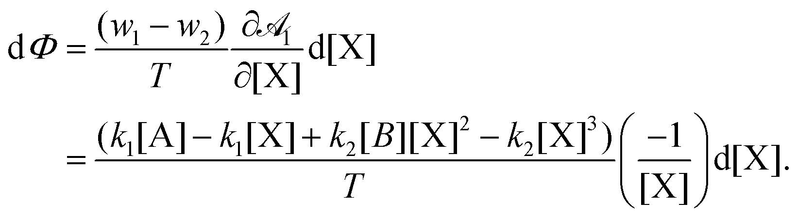


 , which is required for achieving entropy balance at any NESS:
  , see eqn (1).
 and
and  acting on the internal reaction network. The system is then near (far from) equilibrium when
  .
.


 , eqn (8). The lower curve: the exchange entropy per unit volume:
  eqn (24), evaluated at the NESS as functions of the input concentration [B]in. System entropy is balanced on all the NESS:
  , see eqn (1). Units are (J K−1 s−1 L−1). Compare to Fig. 4, for the clamped model, for which there is no exchange entropy.
 for the transition, at [B]in = 0.4, from the unstable NESS to the stable NESS on the upper portion of the bifurcation curves for A and X (and lower portion of the B-bifurcation curve) (see also Fig. 8). Fig. 12 shows the dynamics and the GEC for the transition to the other stable NESS located on the lower portion of the bifurcation curves for A and X (and on the higher portion of the B-bifurcation curve). The behavior of the transitions from the segment of the unstable NESS to either one of the two alternative stable NESS's, is qualitatively similar to the results displayed here. A positive fluctuation in concentration added to either A or to X, or a negative fluctuation in concentration added to B leads to results qualitatively similar to those in Fig. 11. On the other hand, a negative fluctuation added to either A or to X, or a positive fluctuation added to B leads to results qualitatively similar to those in Fig. 12. We have validated the GEC for all these cases. The GEC is obeyed for all the transitions between unstable and stable NESS.

 . Conditions for the existence of a local potential however are given in Chapter IX of ref. 20, but even the existence of a local potential beyond the linear regime is not guaranteed.


 and exchange entropy
 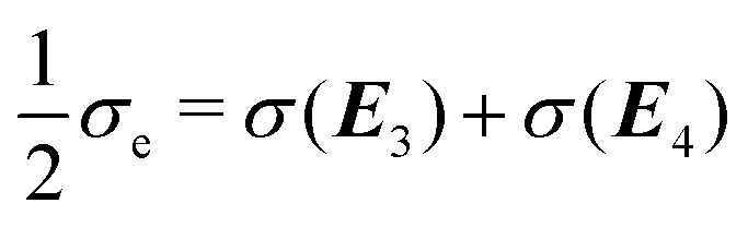 . In contrast to the clamped model, exactly half of the entropy production is distributed over the first two EFMs. And half of the exchange entropy, void in the clamped model, is distributed over the second pair of EFMs; see Fig. 14. The other halves
  are distributed over the final two EFMs, and in a hybrid, or composite, way; as concatenations of one way entropy “productions” and one-way exchange entropies, see Fig. 15.

 . Units are (J K−1 s−1 L−1).
 . The region of unstable NESS bistability and switching is indicated for σ(E6) (σ(E5)) by the pair of red (black) dots. Units are (J K−1 s−1 L−1).
 and σ(E5) = −σ(E6). The latter two EFMs can undergo a mutual switching in their relative ± signs when the system is in an unstable NESS. A compositional fluctuation about the unstable region in σ(E6) (or about the mirror image point in σ(E5)) can provoke a transition to either a greater positive or to a lesser negative value in σ(E6) and correspondingly, to a more negative value or a greater positive value in σ(E5). The latter case gives rise to the switching in signs. The entropy balance is maintained, see Fig. 15. These EFMs E5 and E6 are related by time-reversal. The time-reversal operation flips the direction of the reaction and flow arrows, interchanging forward and reverse transformations, we see that E5 and E6 form a time-reverse pair of pathways. The first four EFMs are then singlets under time-reversal: they transform into themselves under this operation. Note the contrast with models of SMSB whose EFMs can be classified as being either parity (enantiomeric) singlets or doublets.21


