
 Open Access Article
 This Open Access Article is licensed under a
 Creative Commons Attribution 3.0 Unported Licence
Lifting the lid on the potentiostat: a beginner's guide to understanding electrochemical circuitry and practical operation†
Alex W.
Colburn
 a,
Katherine J.
Levey
ab,
Danny
O'Hare
c and
Julie V.
Macpherson
*a
a,
Katherine J.
Levey
ab,
Danny
O'Hare
c and
Julie V.
Macpherson
*a
aDepartment of Chemistry, University of Warwick, Coventry, CV4 7AL, UK. E-mail: j.macpherson@warwick.ac.uk
bCentre for Diamond Science and Technology, University of Warwick, Coventry, CV4 7AL, UK
cDepartment of Bioengineering, Imperial College London, SW7 2BP, UK
First published on 9th March 2021
Abstract
Students who undertake practical electrochemistry experiments for the first time will come face to face with the potentiostat. To many this is simply a box containing electronics which enables a potential to be applied between a working and reference electrode, and a current to flow between the working and counter electrode, both of which are outputted to the experimentalist. Given the broad generality of electrochemistry across many disciplines it is these days very common for students entering the field to have a minimal background in electronics. This article serves as an introductory tutorial to those with no formalized training in this area. The reader is introduced to the operational amplifier, which is at the heart of the different potentiostatic electronic circuits and its role in enabling a potential to be applied and a current to be measured is explained. Voltage follower op-amp circuits are also highlighted, given their importance in measuring voltages accurately. We also discuss digital to analogue and analogue to digital conversion, the processes by which the electrochemical cell receives input signals and outputs data and data filtering. By reading the article, it is intended the reader will also gain a greater confidence in problem solving issues that arise with electrochemical cells, for example electrical noise, uncompensated resistance, reaching compliance voltage, signal digitisation and data interpretation. We also include trouble shooting tables that build on the information presented and can be used when undertaking practical electrochemistry.
1. Why do we care?
Electrochemists typically make two types of measurement. One is a dynamic measurement where a current is measured in response to an applied electrode potential (voltage) e.g. voltammetry, amperometry etc. the second is where the electrode potential is measured between two electrodes (potentiometry), under conditions of negligible current flow. The former requires the use of a potentiostat, which to many starting electrochemists, especially those with little electronics knowledge, is often treated as a plug and play box, without any understanding of the internal workings. Whilst this can suffice on one level, not understanding how the potentiostat works can lead to problems including: possible misinterpretations of the resulting current–voltage signals; experimental errors in making the measurement, difficulties in solving noise problems associated with the system etc. For potentiometry, it may be tempting to measure the voltage using standard laboratory based digital voltmeters (DVMs), however for certain potentiometric systems especially measuring pH using the popular glass bulb electrode,1 the wrong type of DVM will lead to errors. Again an understanding of why this is, is important.This introductory guide thus aims to introduce the starting electrochemist to fundamental electronic circuitry and concepts that underpin voltammetric and potentiometric measurements. In doing so the electrochemist: (i) is equipped with a greater understanding of how these measurements are made; (ii) acquires confidence in problem solving experimental issues; (iii) understands the specifications and suitability of commercially available instrumentation for use in different experimental settings; (iv) understands where noise pick-up can occur; (v) how filters work and; (vi) can interpret the outputted electrochemical data correctly. Table 1 lists a glossary of terms used when describing a potentiostatic circuit; the first time the term is used in the text it is bolded. Tables 2 and 3 are troubleshooting tables covering factors which contribute to Ohmic drop and noise respectively in an electrochemical system, and methods to combat them.
| Term | Definition |
|---|---|
| Voltage | A measure of the difference in electric potential between two points |
| Current | The amount of electric charge passing per unit time |
| Voltage follower | An op-amp circuit which does not produce any amplification to the voltage signal, i.e. the output voltage follows the input voltage. This configuration is used to measure a voltage while drawing negligible current from the source, Fig. 3b |
| Current follower | An op-amp circuit which produces a voltage that is proportional to an input current, whose gain is determined by the selected feedback resistor. Also known as a current-to-voltage (i–E) converter in potentiostat circuits, Fig. 4 and 5a |
| Control amplifier | An op-amp circuit that controls the potential difference between RE and WE by varying the potential on CE using negative feedback, Fig. 3d and 5 |
| Negative feedback | A technique in which a defined proportion of Vout is fed back to the inverting input of an amplifier to accurately set the gain of the amplifier thereby producing an instrumental element capable of accurate measurement |
| Ground | Connects a point in a circuit to 0 V (sometimes called an earth) with very low resistance (≪1 Ω) and as a result maintains the 0 V potential regardless of the current flowing into or out of it. A point possessing these properties provides a stable reference to measure and compare voltages with respect to each other |
| Virtual ground | A point that is not physically connected to ground but maintains its voltage electronically and has the same property of current-invariant potential as a conventional ground. Virtual grounds are generally at 0 V, but can take a finite value |
| Compliance voltage | The maximum voltage that can be delivered by any part of a potentiostat circuit to an electrode or signal output, e.g. control amplifier on the CE and current follower output voltage |
| Source of resistance | Possible solutions |
|---|---|
| Low solution conductivity | (1) If possible, increase the ionic strength of the solution, e.g. with a total ionic strength adjustment buffer |
| (2) Move RE closer to the WE, or use a Luggin probe which is designed to enable very close RE to WE separation5 | |
| (3) Reduce electrode size to decrease the current | |
| (4) Reduce analyte concentration to decrease the current | |
| Poor electrode conductivity | (1) Use another electrode! |
| (2) Reduce analyte concentration to decrease the current | |
| (3) Reduce electrode size to decrease the current | |
| High electrode contact resistance resulting from e.g. corroded crocodile clips | (1) Regularly clean crocodile clips, abrade the connectors with fine emery paper to re-expose metals and wipe down with ethanol |
| (2) Use alternatives to crocodile clips e.g. (i) soldered and insulated connections; (ii) gold plated push fit connectors | |
| Blocked RE frit resulting in increased resistance | A well-maintained frit should have a resistance of around 100 Ω27 but this will rise considerably when blocked. Check the frit regularly and clean or replace as necessary |
| Sources of noise | Noise mitigation strategies |
|---|---|
| Pick-up from power cables, usually identifiable as 50 Hz (UK and Europe) or 60 Hz (USA) and harmonics 100 kHz from switch mode power supplies | (1) Move experiment as far away as possible from power cables |
| (2) Shorten cell and instrument leads as much as possible and keep the cables straight | |
| (3) Use a Faraday cage | |
| (4) Use shielded cables. Unshielded mains or other cables passing into the Faraday cage from nearby equipment e.g. pH meters, can also be problematic even when unplugged from the mains. Therefore consider moving the equipment and cables far from the experiment, when not in use, or enclose all the cables inside the Faraday cage with the equipment | |
| (5) Connect all metals, including clamp stands, helping hands, etc. to a good earth | |
| (6) Ensure any unused connector wires e.g. the second WE/RE connections of a bipotentiostat (when using as a potentiostat) are grounded or at least placed within the Faraday cage and spaced separately | |
| EM-generating equipment e.g. electric motors, switches, etc. | (1) Move external noise sources away from the experiment, where possible e.g. electric motors |
| (2) Unplug any unused high power equipment and move far away | |
| (3) Keep the experiment as far away as possible from digital equipment, such as computers, mobile phones etc. | |
| (4) Use a Faraday cage | |
| Magnetic fields from motors, magnets and high current devices generally | (1) Shorten cables as much as possible and instrument leads |
| (2) Keep cables straight and immobile | |
| (3) Minimize vibration | |
| Ground loops i.e. ground connections made to multiple earthing points | (1) Connect all equipment earths individually to a single point: “star earthing” |
| (2) Get a separate earth connection in the lab for grounding | |
| Poor connections, leaks to earth | (1) Avoid crocodile clips or at least if you are using them make sure they are always clean and corrosion free |
| (2) Use high quality e.g. gold-plated connectors or soldered and insulated connections | |
| (3) Check all connectors for corrosion. Corrosion introduces another electrochemical cell into your circuit | |
| (4) Replace cell leads regularly. Poor connections add resistance and increase noise pick-up | |
| (5) Wipe electrical connectors with alcohol at the start of the experiments to remove moisture | |
| (6) Keep the instrumentation away from electrolyte solutions: a “dry shelf” above the bench | |
| (7) Avoid using dissimilar metals in connectors | |
| Reference electrode resistance | (1) Check the filling solution is topped up |
| (2) Check the frit for blockage. A blocked frit results in an increase in resistance. This in turn slows the response of the potentiostat, increases the susceptibility of the cell to environmental noise (particularly power line noise) and can result in overloads in the system | |
| (3) Check cabling to RE: the higher the resistance of the RE the more it is prone to noise pick-up. It must be shielded at all times | |
| Stray capacitance | (1) Use short cables where possible |
| (2) To minimize stray capacitance when measuring small currents, the electrochemical cell should not be positioned too close to the walls of the cage | |
| (3) Do not run cables close to one another, maintain reasonable spacing as shorter cables will allow |
2. Introduction to voltammetry and potentiometry
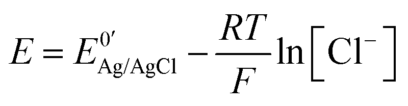
In potentiometry, an electrode potential, E, is measured between at least two electrode/electrolyte interfaces in solution, with at least one being a reference electrode (RE). The Nernst equation is used to relate E to the concentration (or strictly activity) of potential determining ions in the solution. In redox voltammetry, an applied E is used to drive faradaic electron transfer i.e. oxidation or reduction, of a redox species at the surface of a working electrode (WE), resulting in a current flow, i. WE's are electrically conducting electrodes of known material composition and geometry e.g. metal or carbon disc electrodes with a surrounding insulating sheath. As E cannot be applied to one electrode alone, there has to be a second in solution to complete the circuit. This electrode is the RE. E is thus reflective of this potential difference between WE and that of a fixed reference point, the RE, measured in volts.2,3 As the RE potential is constant, any change in E appears across the WE–solution interface only, isolating the WE as the electrode under investigation.There are many excellent reviews and articles written about RE's and the purpose here is not to discuss them in detail, we simply highlight key features of importance for this article.4,5 In particular, the potential of the RE, governed by the Nernst equation, ideally should not change even if a small current flows across the electrode–electrolyte interface; this property is referred to as non-polarizability. However, whilst no electrode truly fulfils this condition, there are some which come close and are characterized by very high electron transfer rate constants. Popular RE's include metal/metal halide/halide ion systems, for example silver chloride coated Ag wire in contact with a chloride solution (Ag|AgCl|Cl−) and the calomel electrode (Hg|Hg2Cl2|Cl−), mercury in contact with solid mercurous chloride, also in contact with a chloride solution. For the Ag|AgCl|Cl− RE, which undergoes electron transfer in accordance with eqn (1), applying the Nernst equation results in eqn (2):
| AgCl (s) + e− ⇌ Ag (s) + Cl− | (1) |
 | (2) |
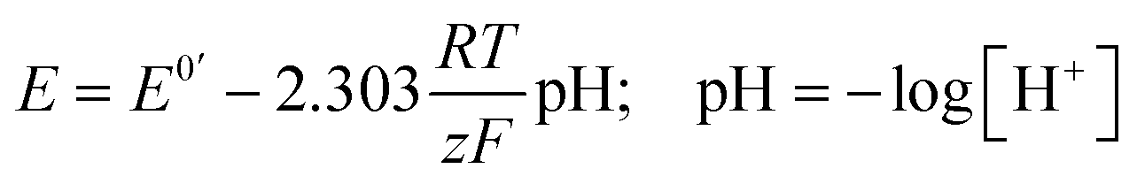
For potentiometric applications, the analyte of interest can only be measured accurately if the RE potential is stable. Consider the glass bulb pH electrode which contains two REs either side of a thin glass membrane. Differences in proton concentration across the membrane results in a potential difference which varies logarithmically with [H+] in accordance with eqn (3):
 | (3) |
 | (4) |
In voltammetric experiments the RE stability requirements are dependent on the measurement made. For example, if a peak potential is being used to identify an analyte then its determination to ±5 mV would usually be more than adequate. In contrast for electron transfer kinetic analysis the requirements are much more stringent. In voltammetry as a current always passes, to provide a stable RE reading with no time-dependent drift, then ideally no current should flow through the RE. Current flow results in perturbation in the concentration of the potential determining ion via e.g.eqn (1). The same is true of a potentiometric circuit. Whilst it is normally considered in potentiometry that negligible current is flowing when you measure an electrode potential, it is important to consider that under some circumstances this might not be the case. A small current flow coupled to high resistance in the circuit, can lead to problems.
In fact for any circuit which has current flowing it is important to consider the impact of Ohmic drop (or loss). It arises as a consequence of Ohm's Law which states that a voltage is required to move current through a resistive component of an electrical circuit. Our electrical circuit is the electrochemical cell, and there are many factors which contribute to the resistance. Moving current through this resistance results in voltage “lost” from that which is applied. Most potentiostats are used under conditions where the potentiostat is unaware of Ohmic drop and will output a value believed to be the applied electrode potential. However, if Ohmic drop is significant, the potential the WE experiences (versus the RE) is actually less than the value the potentiostat outputs. This leads to problems in correctly interpreting the data. When measuring an electrode potential, one way to avoid Ohmic drop is to use a measuring device which has a high internal resistance, so that negligible current flows. The common laboratory DVM, which has an internal resistance of ∼10 MΩ, suffices for many applications. However, as shown later, this approach is not appropriate when measuring the electrode potential associated with the glass bulb pH electrode.
In voltammetry, the current generated at the WE must flow somewhere. To prevent current flow through the RE, an alternative current path is provided through the use of a third electrode, called the counter electrode (CE). The same magnitude current flows through the CE as WE, but is opposite in direction. The voltage applied to the CE is typically not outputted automatically by most potentiostats but is accessible. It is possible to use a two electrode set-up comprising WE and RE (where the RE serves as both a RE and CE) but only if small currents are passed through the RE in order to prevent a measurable change in the potential across the RE–electrolyte interface. This is achieved when working with WE's in the micro- and smaller regime. See SI 1 (ESI†) for an estimation of the maximum current that should be passed in a two electrode system.
Thus in the conventional voltammetric three-electrode set-up, E is controlled between WE and RE and current passes between CE and WE. The set-up can be represented schematically in many different ways, for example as shown in Fig. 1. The output of this experiment, a voltammogram, typically plots i on the y axis and E (vs. RE) on the x axis. This experiment is carried out using a potentiostat, first introduced in 1942 by Archie Hickling (University of Leicester, UK),9 which for many electrochemists is bought from a commercial entity and is often operated as a plug and play device. There are many different commercial potentiostats on the market today. There are also less sophisticated, home-built potentiostats now being described more routinely in the literature, which can prove useful for many applications.10–12 Lifting the lid off the commercial potentiostat and working to understand every component along with its function can prove confusing and is time-consuming for a starting electrochemist. However, there are certain key concepts which hold true for all systems. Reading this article, we hope, will give you confidence in your understanding and encouragement to have a go yourself.
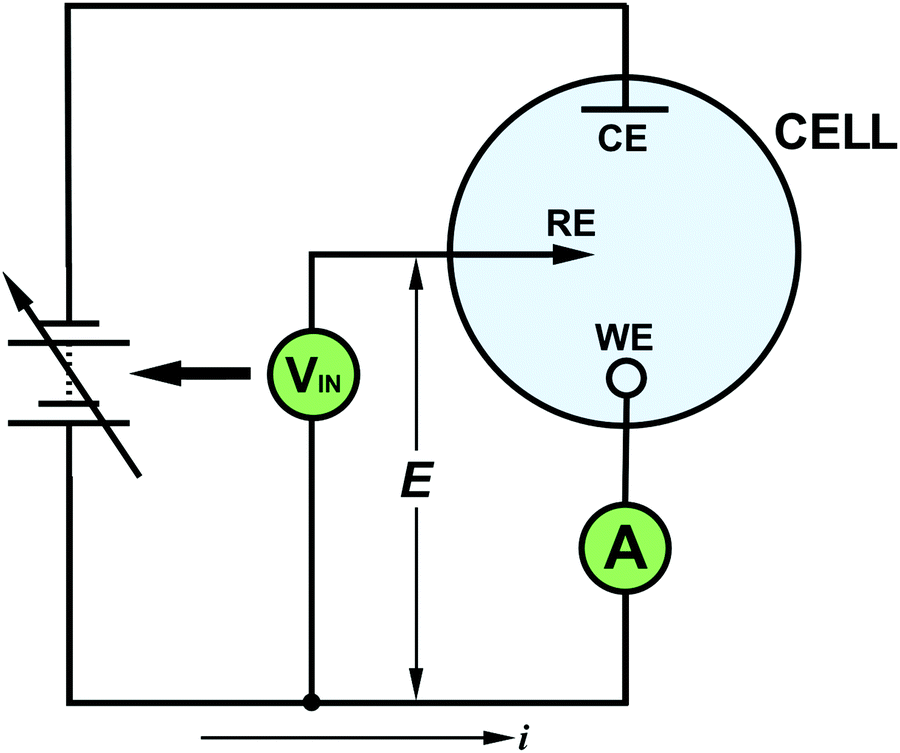 | ||
| Fig. 1 Schematic of a typical three electrode electrochemical set-up, with the appropriate symbols used for WE (O), RE (arrow) and CE (⊥). Current flows between CE and WE whilst E is controlled between WE and RE. | ||
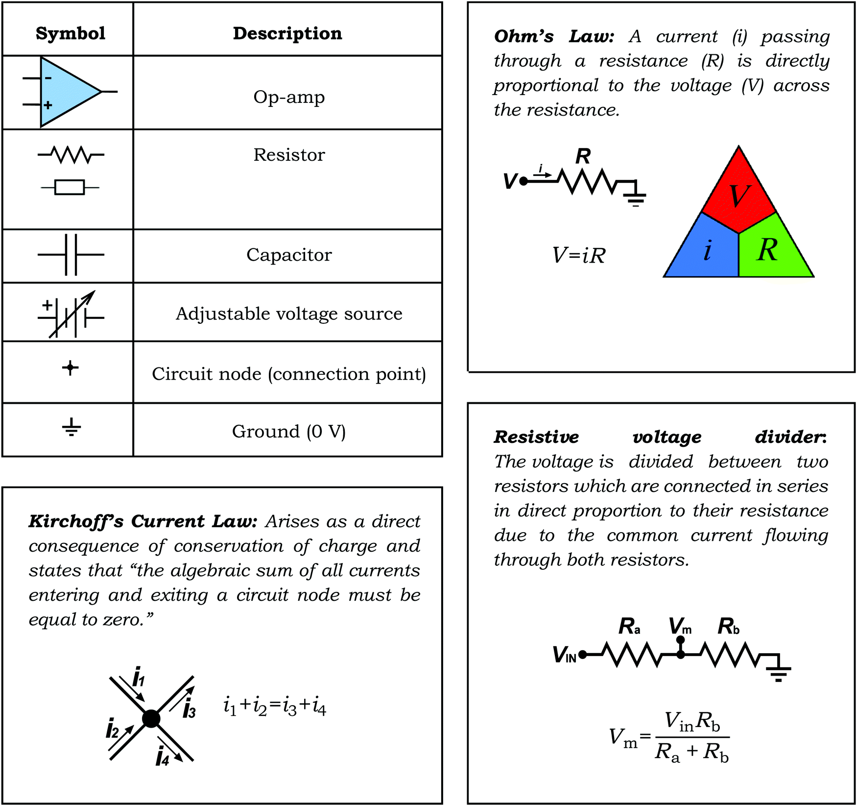
3. Electronic symbols of importance
In this section we introduce the electrochemist to electronic symbols and highlight simple yet important electronic circuits and concepts; Ohm's Law has already been introduced. We describe an important electronic component critical in potentiostat design and potential measurement: the operational amplifier, referred to as op-amp. The circuits will be described in terms of their application in a potentiostat and electrochemical potential measurement. Box 1 details seven electronic symbols that an electrochemist should be familiar with and highlights electrical laws/rules that are often used when interpreting electrochemical cells and circuits; Ohm's Law, Kirchoff's Current Law and Voltage Divider Circuits. Note, (i) for the resistor we have included two symbols as both are commonly used; each has been approved by a different electrical standards organisation. (ii) When using Ohm's Law, the symbol V is used for voltage as this applies to all electrical circuits.The op-amp is the principal active component of all electrochemical instrumentation. The op-amp is so named because of the devices developed for use in 1960's analogue computers, which were used to simulate the function of mathematical operators, for example addition, subtraction, integration and differentiation.13 Though the original devices were built from discrete electronic components, modern op-amps are integrated circuits with many components miniaturized onto a single silicon die. The electronic symbol for the op-amp is given in Box 1.
The op-amp has important characteristics, highlighted in Fig. 2. Note, as shown in Fig. 2, two vertical negative and positive power supply connections are often added to the op-amp symbol as they are required to operate the op-amps internal circuitry. An op-amp has two voltage inputs and one voltage output. The two voltage inputs are very high resistance, typically >1012 Ω in order to draw negligible currents and prevent loss of voltage due to Ohm's Law. In this article, we use resistance rather than impedance as all the electrochemical applications discussed are effectively dc i.e. where the current/voltage is not continually varying from positive to negative (impedance is an ac resistance). The output is low resistance, generally less than 100 Ω, typically down to 1 Ω for most applications, meaning current can easily flow from the output. The two voltage inputs are labelled + and − and are referred to as the non-inverting input (+) and inverting input (−) respectively. Vdiff defines the difference in voltage between the two inputs = [Vin(+) − Vin(−)].
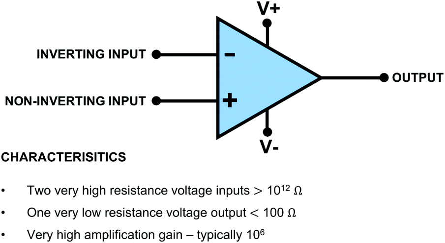 | ||
| Fig. 2 Symbolic representation of an op-amp and key characteristics. | ||
Op-amps have characteristic high gain values (G). This is an amplification factor and is defined by eqn (5) where Vout is the output voltage.
 | (5) |
The most common method of operating the op-amp is in the feedback mode; all the circuits discussed below are feedback circuits, where the output voltage is fed back to one of the voltage inputs. Due to the high gains, to keep the output voltage within an operable range the two input voltages must always be kept extremely close in value. For example, for a typical 106 gain op-amp, this means not exceeding a voltage difference across the two inputs of ±0.015 mV to prevent an operating voltage of ±15 V being exceeded. Given voltages are at best measured with an accuracy of 0.1 mV, using a standard laboratory based DVM, for practical operation in a feedback circuit the voltage inputs of an op-amp are effectively maintained at the same voltage. This concept is very important and will help when interpreting the op-amp circuits in this article.
4. Measuring voltages
It was highlighted earlier that a standard lab based DVM (often at the cheaper end of the market) would not suffice to measure the potential difference across a glass bulb pH probe. We now provide an explanation as to why and introduce an op-amp voltage measuring circuit. In the glass pH probe the highest resistance component results from the thin glass membrane, Rp, with values typically between 50–500 MΩ;14,15 the thinner the membrane the lower the resistance. These high values create a problem, Rp is now greater than that of the internal resistance, RM, of a typical laboratory DVM (ca. 10 MΩ). To illustrate this in more detail, consider the worst case scenario which is measuring the voltage across the 500 MΩ glass pH membrane using a 10 MΩ DVM. Fig. 3a shows a typical circuit to do this where the glass probe is in series with the DVM. At pH 6, if the system produces a voltage of, let's say, +59.16 mV at 298 K, we can use Ohm's Law to calculate the current flowing. As the total resistance in the system is Rp + RM and the voltage is +59.16 mV, the current flowing through the DVM and pH probe = 116 pA (most likely arising from the redox processes associated with the two RE's).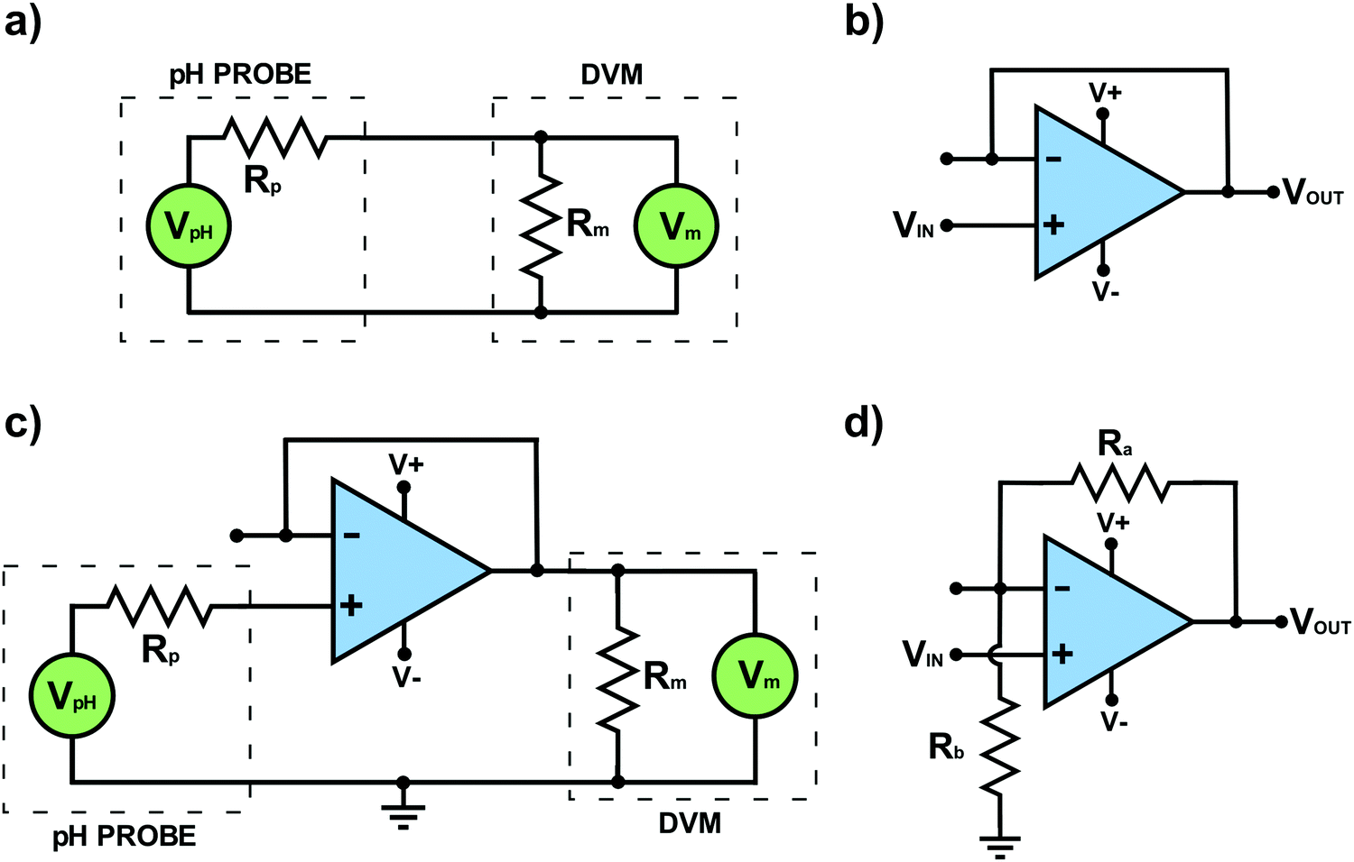 | ||
| Fig. 3 Schematic diagrams showing (a) circuit for measuring the pH at a potentiometric glass probe using a DVM only; (b) voltage follower op-amp circuit; (c) circuit for measuring pH using an op-amp voltage follower circuit (d) amplification using a negative feedback loop op-amp circuit. The semicircle in the line running from the node point (+) at Vin(−) to ground through Rb indicates that the wire is not connected to Vin(+) and simply passes over it. | ||
On the face of it this current seems very small and unproblematic. However, the current has to flow through both resistors associated with the DVM and the glass pH probe, with the total voltage across both resistors equalling +59.16 mV. Considering the voltage divider circuit in Box 1, we can work out how much voltage is dropped across each resistor. In this case given the much higher resistance of the glass probe compared to the DVM (×50) almost all the 59.16 mV voltage is now dropped across the glass membrane = 58.00 mV, with only the remaining 1.16 mV registered across the DVM. As the resistance of the membrane increases the situation worsens. As the DVM now reads 1.16 mV it erroneously reads a pH value nearer to 7 than 6, a whole order of magnitude error in the determination of [H+]. The system has experienced a form of Ohmic drop. To prevent such errors, one way is to use a very expensive DVM with a much higher internal resistance e.g. 1013 Ω, so that virtually all the voltage now drops across the DVM and not the glass membrane resistance.
Voltage follower op-amp circuit
However, as we shall now show this is completely unnecessary when a considerably cheaper op-amp circuit that works to precisely measure the voltage can be adopted for glass bulb pH potentiometric measurements. Using the concept of negative feedback it is possible to build a simple voltage follower op-amp circuit that can do the required job. Here the circuit works such that the input voltage to the op-amp is the same as the output voltage. This may on the face of it, seem like a rather pointless activity. Why employ an electronic circuit that does this? If the potential established at the glass pH probe could have been fed to the voltage input of this op-amp circuit and a DVM connected to the output, the output voltage would now correct itself to ensure that the DVM measures the same voltage as that generated at voltage input (=the pH probe). The question is how does the op-amp circuit do this?Fig. 3b shows the voltage follower circuit which is also called a “buffer with unity gain”. The input voltage is fed into Vin(+) and Vout is fed back to Vin(−). To satisfy the feedback operating requirement that both voltage inputs must be at effectively the same voltage, any voltage applied to Vin(+) drives Vout to a value where Vout equals Vin(+). Note, as Vout is typically within a few μV of Vin(+), it is appropriate to say that the two voltages are effectively the same. For completeness, as voltages should always be defined between two points, in Fig. 3b the input voltage is applied between Vin(+) and zero volts (called ground); in Fig. 3b the ground symbol has not been shown. Vout is also that between Vout and ground. A discussion on ground and virtual ground is given in Table 1. The voltage follower circuit has the advantage of very high internal resistance (negligible current flows) and at the same time provides a low resistance output to drive measurement instrumentation.
Fig. 3c shows a typical pH measuring circuit which employs a voltage follower op-amp circuit. The op-amp is used as an interface between the glass pH probe and the DVM. The glass pH probe registers a potential, which is input into Vin(+), whilst the output (Vout) is fed into the DVM. In this negative feedback mode, the DVM is now accurately measuring the potential established at the pH probe, as any voltage loss due to a current flowing through Vout and RM of the DVM, has been corrected for. Further information on electronic circuitry for open-source pH instrumentation is given in ref. 16 and 17. Voltage follower circuits are also ideal for use in other potentiometric measurements. A 10 MΩ laboratory based DVM is only appropriate in situations where the resistance of the potentiometric electrode system is significantly lower than that of the internal resistance of the DVM. If using a 10 MΩ DVM also beware blocked frits on e.g. commercial RE's, as they result in much higher probe resistances than expected.
In order to measure small voltages, typically mV's, a more flexible adaptation of the negative feedback circuit is required, which incorporates resistors in a “feedback loop” in order to amplify the measured output voltage, as shown in Fig. 3d. The loop running from Vout to ground (0 V), in Fig. 3d contains a voltage divider chain of two resistors, Ra and Rb. This has the effect of supplying a known fraction of Vout to Vin(−). As shown in Box 1, Ohm's Law governs the effect of the divider chain and enables the voltage drop across each resistor to be calculated. For example, consider the case where Ra and Rb are the same. If we imagine an input voltage, Vin(+) of +1 mV, due to the divider chain in the feedback loop only half the voltage at Vout will appear at Vin(−). As the op-amp functions to maintain its inputs at the same voltage, Vout must therefore increase to +2 mV in order to deliver +1 mV at Vin(−). This circuit has a voltage gain (Gv) of two, with GV defined by eqn (6), where Vin is the voltage at Vin(+).
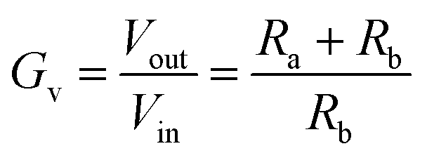 | (6) |
5. Measuring current
There is one other feedback op-amp circuit to highlight before considering the circuits which are useful in a potentiostat and that is one that can be used to measure a current as shown in Fig. 4. This type of circuit is usually referred to as a current to voltage converter or “current follower”. Here Vin(+) is directly connected to ground (0 V) and thus, via the operating principles of the op-amp in feedback, the node point (see Box 1) connected to Vin(−) is also held effectively at “virtual” ground. We use the term virtual (see Table 1) as this point is not directly connected to ground. All previous op-amp circuits have been analysed in terms of voltages appearing at their various terminals. However, when one of the inputs is directly connected to ground or virtual ground the circuit must be analysed in terms of the currents flowing in the surrounding circuit since analytically descriptive voltages no longer appear at the inputs.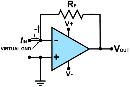 | ||
| Fig. 4 Op-amp current to voltage converter (current follower) circuit. | ||
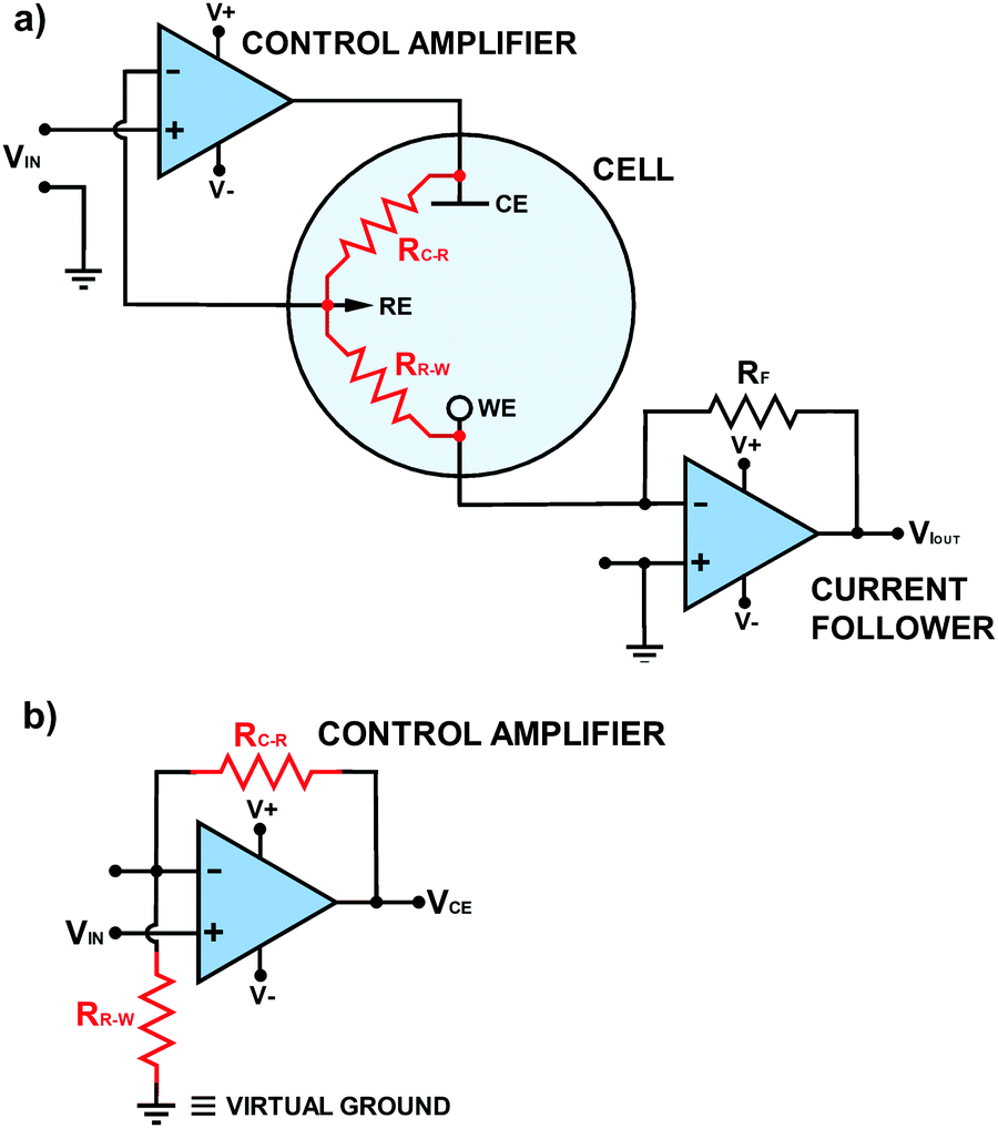 | ||
| Fig. 5 (a) Electronic circuit version of Fig. 1 including solution resistances between RE and CE (RC–R) and RE and WE (RR–W). Other resistances also contribute to RC–R and RR–W but are not explicitly shown on this diagram. (b) The control amplifier circuit presented in the same form as Fig. 3d, where VCE represents Vout. | ||
In Fig. 4 current flows into the virtual ground node point at Vin(−); there is a negligible current flowing into the Vin(−) input itself due to the extremely high resistance of the input. Kirchhoff's current law (Box 1) states that the algebraic sum of all currents entering and exiting a node must equal zero. If the current flowing into the node point is positive a negative counteracting current must flow out of the node point. To produce this negative current, in accordance with Ohms Law, Vout moves to an appropriate negative value dependent on the magnitudes of RF and the current. Hence Vout is inverted in sign with respect to the current flowing into the input.
6. Potentiostatic circuits
Now let's consider the requirements of a potentiostatic circuit and how op-amps can help. A known potential difference must be applied between the WE and RE and the current flowing through WE must be appropriately recorded. Wherever possible Ohmic drop is accommodated. This can be achieved using two op-amp circuits as shown in Fig. 5a.As these circuits also now represent the real system there are two electrochemical cell resistances to take note of, one which exists between RE and CE (RC–R) and the other between RE and WE (RR–W), as shown in red in Fig. 5a. These resistances contain contributions from the solution resistance between the two electrodes but also charge transfer resistance (Rct) associated with either the WE, CE and RE electrode/electrolyte interfaces. Other contributions are highlighted later in Table 2. Solution resistance is governed by the electrolyte concentration, electrical mobility of the ions in solution and the separation/area of the appropriate electrodes,18 whilst Rct is dependent on the ease of electron transfer of a redox analyte; the higher Rct the slower the electron transfer kinetics.
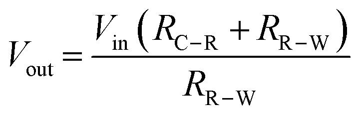
To a starting electrochemist it is often tempting to think that the potential is applied directly to the WE, but in most potentiostats, the desired potential is applied (indirectly) to the RE (see Fig. 5a) and the WE is held at a virtual ground (if you trace back to the WE connection). The op-amp circuit that controls the RE potential is referred to as the control amplifier and is a negative feedback circuit. It is very similar to the circuit described in Fig. 3d, but with Ra replaced by RC–R and Rb replaced by RR–W, as shown in Fig. 5b. The desired voltage is input into Vin(+) and RE is connected to Vin(−). Vout is connected to the CE. Current flows from the CE through both RC–R and RR–W to WE. These two resistances form a potential divider circuit with RE at their junction. The voltage between Vout and Vin(−) contains the resistor RC–R, whilst RR–W lies between Vin(−) and virtual ground. Depending on the ratio of the values of RC–R and RR–W to RR–Wthe op-amp adjusts the potential on the CE (Vout) until the RE electrode voltage attains a value equal to the desired Vin(+), eqn (7), in accordance with eqn (6). Depending on the magnitude of RC–R, Vout can be ∼equal to Vin (if RC–R is negligible) but is normally larger.
 | (7) |
As the op-amp maintains the voltage at RE equal to Vin(+), it automatically compensates for any changes in the resistance of RC–R, due to RC–R being in the circuit between Vout and Vin(−). Unfortunately this also means the op-amp is blind to changes in RR–W, as in this part of the circuit the potential difference is simply maintained, irrespective of RR–W; we will return to this point later as it is very important when interpreting real data. An additional problem arises if the RE is disconnected with the potentiostat still applying a potential; the same arises if you have a very poor contact to the RE. The control amplifier circuit can no longer see a potential on the RE, considers it to be zero, and applies higher and higher potentials up to the maximum of the power supply unit. This can have devastating consequences for your WE which experiences, as a consequence, the full potential capabilities of the potentiostat. The current response will also be seen to flat-line.
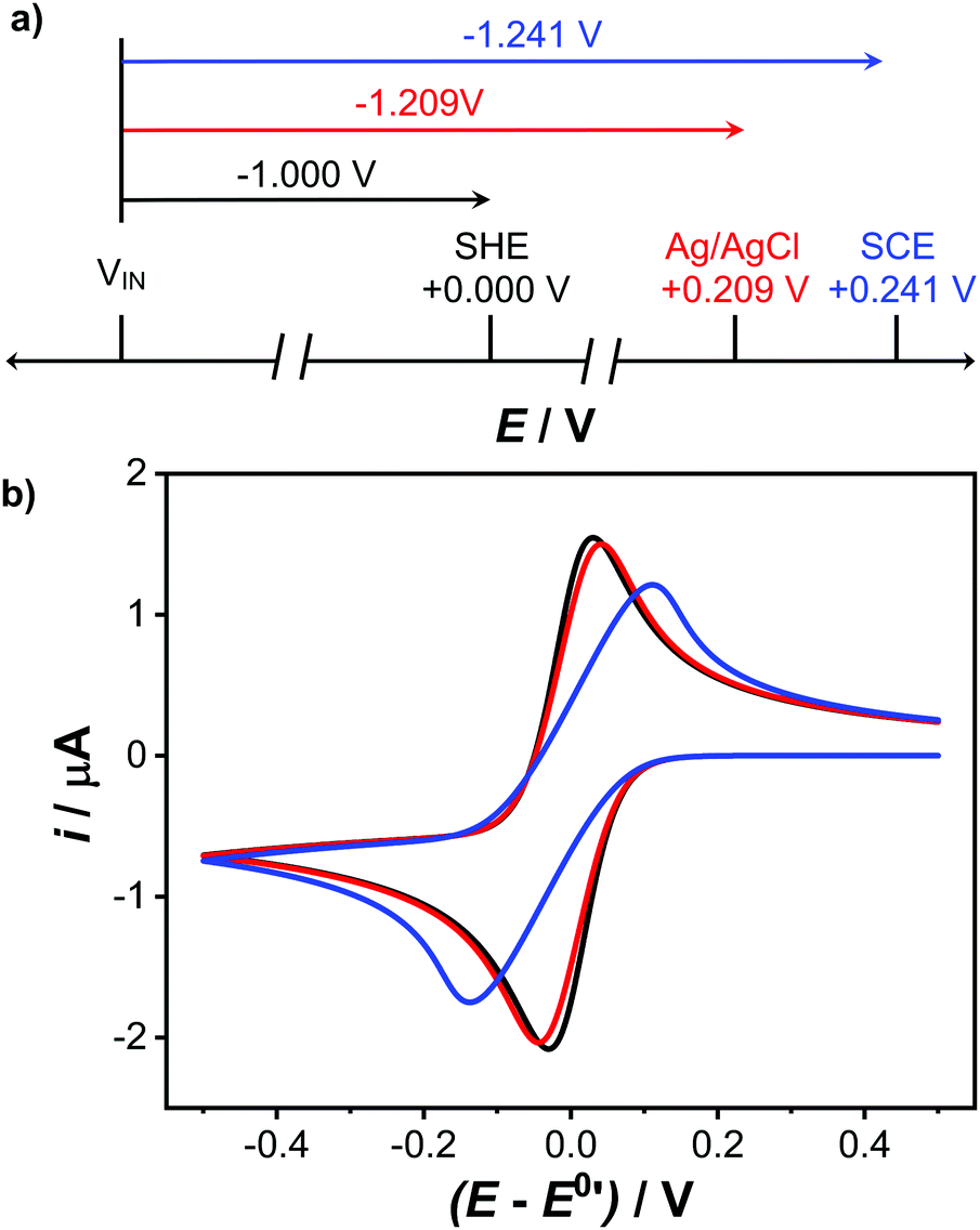
One further important point. As each RE already has its own intrinsic potential, when the external voltage source supplies a known voltage to the RE, this value is added to its intrinsic potential, as shown in Fig. 6a. This is why it is necessary to shift the position of a voltammogram along the potential axis, when comparing the same voltammetric system recorded with different RE's. For example, if we assume the RE is held at an input voltage of +1.000 V, versus the WE held at ground (0 V), for a standard hydrogen electrode, SHE (=0 V), E (WE vs. RE) = −1.000 V. However, if we use an Ag/AgCl RE = +0.209 V for 3 M Cl−, E is −1.209 V, whilst for a SCE = +0.241 V, E = −1.241 V.19
 | ||
| Fig. 6 (a) Comparison of WE vs. different RE potentials for an input voltage of +1.000 V, (b) the reduction of 1 mM [Ru(NH)3]3+ at a 1 mm diameter disc electrode, simulated using COMSOL Multiphysics 5.5™ for no uncompensated resistance (black), Ru = 5 kΩ (red) and 50 kΩ (blue) Full details of the simulation can be found in SI 2 (ESI†). | ||
The control amplifier has a maximum Vout, which is known as the compliance voltage, this is the maximum voltage of its power supply (e.g. ±15 V). If reached the control amplifier will overload, resulting in a flat-lined current response. What may cause the control amplifier to reach compliance? One of the main reasons is if RC–R is significant and the user is trying to access high potentials; Vout is forced to higher potentials to accommodate the higher RC–R, see eqn (7). Solutions of low conductivity or low dielectric constant will result in high RC–R values, along with the use of electrodes which show a high Rct. Using high conductivity solutions and/or electrocatalytically active (low Rct) CE's such as Pt-black on Pt,20 help in preventing the compliance voltage being reached. Switching to a far less electrocatalytically active electrode material, such as boron doped diamond,21 will increase Rct and thus result in larger Vout values. Reducing the area of the CE with respect to the WE also results in increased resistive contributions as a result of the same magnitude current being forced through a smaller electrode area. This is why CE's of areas typically much bigger than the WE are recommended.
Accessing the voltage on the CE (Vout) is useful in order to understand how hard the CE (Vout) is working, whilst also providing information on which electrochemical reactions may be contributing to the CE current. For example, knowing Vout is at a potential where water breakdown occurs is important since this will lead to changes in pH (if unbuffered) and generation of oxygen or hydrogen; although bubble formation does provide a visual clue of CE potential. If oxygen is present in solution, and the WE reaction is oxidative, then it is highly likely a component of the CE reaction will be oxygen reduction. Depending on the CE material, this can result in hydrogen peroxide formation.22 Production of unwanted CE products is one of the reasons placing the CE behind a glass frit should be considered, although this may introduce more resistance (to RC–R) into the system. For some electrochemical applications such as e.g. electroplating, electrosynthesis,23 the use of pouch cells in battery research, where high potentials are needed, it may be necessary to use potentiostat op-amps with much higher compliances and current capacities.
To measure the current flowing through the WE it is necessary to convert it to a voltage. This is important since the vast majority of recording devices e.g. computers, only log voltages, not currents. An added bonus of converting the current from a high resistance electrical cell to a low resistance voltage source is a reduction in noise pickup. To do this a current follower circuit is adopted as shown in Fig. 5a. For the circuit given, the output voltage has the opposite polarity to the input current. The circuit could be modified further by adding an inverting amplifier to restore the correct polarity. However, it is beyond the scope of this article to describe all electrochemically useful op-amp circuits in detail and the interested reader is instead directed to ref. 24 and 25 for further information. The value of RF on the current follower determines the range of input currents that can be measured. For example, a 1 MΩ resistor gives a current sensitivity (referred to also as a current gain) of 1 μA V−1 whereas a 1 GΩ resistor gives a current sensitivity of 1 nA V−1. The maximum output voltage (compliance) governs the maximum current that can flow. By employing different RF's one potentiostat can operate over nA to mA current ranges, with the same output voltage range. The potentiostat simply selects a current range by switching between different RF values.
Whilst it is always possible to measure a current by passing it through a resistance and simply recording the voltage drop, using for example an instrumentation amplifier, there is a significant advantage to using the op-amp current follower and related circuits. In particular, WE is kept at virtual ground which makes it possible to measure low currents accurately without having to take exceptional and expensive engineering precautions. Furthermore, since the WE is at the same potential as ground, short circuits to earth, which can arise from having electrolyte films on the electrode leads, for example, present less of a problem, as currents can only flow between points at different electric potentials.
So having achieved both a user-defined potential difference between the RE and WE and established a way to measure the current passing through the WE there is still one outstanding issue for the electrochemist to consider, RR–W. This resistance contains Rct and solution resistance but also other resistances not associated with electron/ion transfer, collectively referred to as the uncompensated resistance, Ru. Current passing through Ru, results in an Ohmic drop, and is not compensated by the potentiostat circuit, unlike RC–R. This is true of the circuit in Fig. 5a and most commercial potentiostats unless they explicitly state they have added an additional feedback compensation circuit.26
Thus in a real electrochemical cell, Ohmic drop must be considered, eqn (8).
| E = EWE − ERE + iRu | (8) |
Sloping CVs, poorly formed peaks, peak–peak potential separations for reversible couples >57 mV/n, peak widths at half-height >59 mV/n (where n is the number of electrons passed)28,29 and excessive noise are all indicators that you may be having Ru issues. As a potentiostat user it is thus always recommended to have an understanding of Ru for your system. A common way to quantify Ru includes recording a non-faradaic charging current, ic–time curve in electrolyte-only conditions in response to a potential step of ΔE,28,30 where eqn (9) applies ic, is characterized by the time constant (RuCdl in seconds) where Cdl is double layer capacitance.
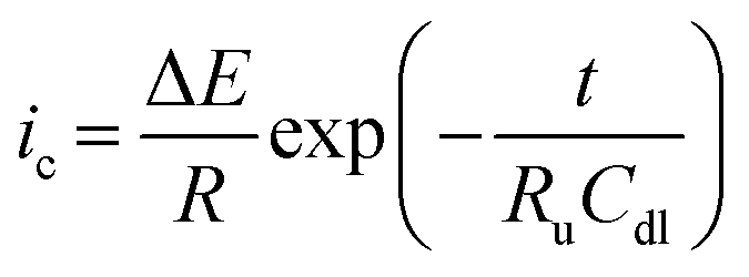 | (9) |
The vast majority of potentiostat users will employ three electrode systems. For electrochemical systems where small currents are passed e.g. when using micro/nano electrodes,32,33 for e.g. the measurement of fast electron transfer kinetics, spatial mapping of surface (electro)chemical activity,32,33etc. it is possible to use two electrodes. Here the RE serves as a quasi RE/CE electrode, and as only small currents flow through the RE, it is possible to maintain a stable potential (SI 1, ESI†). Practically, a potentiostat can be used and the CE/RE leads connected to the RE or bespoke electronic circuitry can be designed and employed. SI 3 (ESI†) shows an exemplar op-amp circuit diagram for a two-electrode set-up.
7. Signal conversion, processing and noise
Whilst the above has provided an understanding of how a potentiostat works and insight into experimental factors which must be considered when setting up the electrochemical cell, it is prudent to highlight three other aspects of experimental electrochemistry linked to potentiostat use. (1) How the output current and voltage signals are recorded digitally for the user; (2) what causes noise on these signals and how to combat noise and finally; (3) use of filters in the potentiostat for removing noise.Signal conversion techniques
The most common technique encountered by the electrochemist is CV and signal conversion techniques are illustrated using CV as a guide. The potentiostat records three variables: (1) Vout which is proportional to the cell current (Vout = iRF); Fig. 5a, (2) the applied voltage, Vin(+) which equates to E (vs. RE) and (3) the time, t, at which these values are recorded. The electrochemical cell outputs analogue signals i.e. continuous signals that vary in amplitude and frequency (time) without quantization, in theory allowing for an infinite number of i, E and t values to be represented.In the early years of electrochemistry, the cell was controlled with analogue instrumentation e.g. triangular wave generators using an integrating op-amp circuit and the outputs recorded on chart recorders. This approach resulted in truly linear potential ramps, defined by a constant voltage scan rate, v in V s−1, and was the method that underpinned the seminal theory of linear sweep and CV.29 Desktop computers have now moved the experiment to the digital domain, which means a finite, not infinite, set of values, for time, current and voltage. Understanding the digitization process and its relationship to the analogue electronics is thus vital for obtaining useable data that is correctly interpreted. For the electrochemist it is important that the digitized points for i and E are recorded close enough together to enable a reliable estimate of the position of the maximum of a peak and its value. This requires optimization of the sampling rate i.e. how frequently the measurement can be taken, and an understanding of the maximum number of data points that can be recorded. The latter is governed by the maximum file size. An understanding of Nyquist sampling theory is also important, which states that in order to obtain a faithful representation of data, you must sample at least twice as fast as the highest frequency component of that data (we will return to this later).13 Furthermore, since the process of digitization leads to discrete steps in the data, it is also essential to optimize the potential step size and the gain of the current to voltage converter i.e. i to V setting, so that these steps are insignificantly small.
In a typical CV experiment the digital computer will generate a data stream for the potentiostat to convert into a varying voltage waveform, where the voltage is increased linearly with time and then decreased, resulting in a triangular voltage waveform. This is sent to the input of the potentiostat's control amplifier (Fig. 5a). The process requires a digital to analogue converter (DAC), whereby digital numbers, generated by the computer, are used to reproduce this waveform and are converted to voltages with respect to the input number, using a technique called digital frequency synthesis. The resulting output from the DAC consists of a series of discrete voltage steps timed to approximate the waveform shape. Note the output is not strictly analogue in the truest sense, it serves as an approximation, which approaches ideality as the number of data points increases and time taken to complete each digitization (conversion rate) decreases. The computer must also acquire (sample) and store the resulting i versus E(t) data. This requires the continuously varying analogue i versus E(t) data to be converted to digital numbers for storage; analogue to digital conversion (ADC). The choice of DAC/ADC is important as it impacts the maximum number of data points that the potentiostat can record, the conversion rate (DAC) and the sampling rate (ADC). Having an understanding of ADC/DAC is thus extremely helpful.
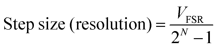
The maximum number of discrete voltage data points a potentiostat can deliver is governed by the bit depth of the DAC/ADC convertor. In theory a DAC/ADC can have any integer bit depth but the most commonly encountered have 8, 12, 16, 24 or 32 bits, where the number of data points (or steps) associated with N bits is 2N. For example, an 8 bit DAC/ADC has 28 = 256 points, whilst a 16 bit has 216 = 65![[thin space (1/6-em)]](https://www.rsc.org/images/entities/char_2009.gif) 536 points and therefore improved measurement resolution. The potentiostat will also have a maximum full-scale voltage range (VFSR) that it can work over, again governed by the DAC/ADC used. The smallest voltage resolution (smallest step size) of the potentiostat is intrinsically linked to VFSR and bit size and is given by eqn (10).
536 points and therefore improved measurement resolution. The potentiostat will also have a maximum full-scale voltage range (VFSR) that it can work over, again governed by the DAC/ADC used. The smallest voltage resolution (smallest step size) of the potentiostat is intrinsically linked to VFSR and bit size and is given by eqn (10).
 | (10) |
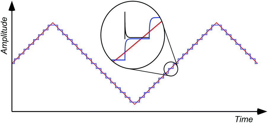 | ||
| Fig. 7 4 bit digitally synthesized triangular waveform. On this scale the 16 bit waveform would appear indistinguishable from the straight lines of the triangular waveform. The insert shows an individual current–time decay curve which is the result of the potential step applied. | ||
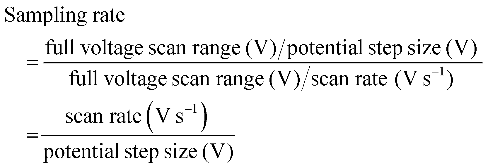
In CV the user is always asked to input start potential, voltage limit, number of cycles and scan rate. In some systems step potential is also requested, if not the potentiostat automatically sets this value based on the scan rate inputted. From these values the sampling rate can be determined, i.e. the number of data points recorded per second (in Hz), as shown in eqn (11). Having knowledge of the sampling rate is important, especially when it comes to understanding the impact of noise (discussed later) on the data. For most commercial potentiostats, the sampling rate is not explicitly specified.
 | (11) |
For example, consider a CV where the potential is scanned at 0.1 V s−1 from 0.0 V to +1.0 V and back; a full voltage scan range of 2.0 V which takes 20 s. If a potential resolution (step size) of 1 mV is chosen (typical for this scan rate) this means recording 2000 data points for current (and E) in 20 s, which equates to a sampling rate of 100 Hz. As eqn (11) shows, doubling the scan rate or halving the potential step size results in a doubling of the sampling rate to 200 Hz.
The staircase nature of the CV also means that for each step in potential, an i–t curve is obtained (see inset to Fig. 7). The potentiostat will analyse the current over some part of this curve, this could be at the end of the step, or averaged over a defined percentage of the step; some potentiostats offer the option of choosing where the current is sampled on the i–t curve. A single current measurement per potential step is reported, but this will differ between commercial potentiostats depending on where sampling takes place so it is useful to know how your potentiostat samples, especially if you are seeing slightly different data recorded using different potentiostats. The question is does this matter? To address this it is useful to consider experimental results which compare digital staircase to linear (analogue) scans. Whilst this topic warrants a review in its own right the salient points are featured here. For a simple reversible, solution phase redox system, recorded at a macroelectrode, it has been shown that noticeable differences are observed when staircase currents are sampled at the end of each potential step.34,35 Ref. 36 summarizes the results of comparative studies. The situation is often worse when CVs for surface-bound processes are recorded e.g. Hads/des on Pt37 or surface-bound redox electrochemistry.38,39 For example, depending on where sampling takes place, digital staircase voltammetry can over or under estimate the true Cdl or surface coverage of species, compared to linear scan voltammetry. It has been shown that for certain systems averaging the current over the entire i–t curve can produce similar results to linear scan CV.40 Most commercial potentiostats do offer add-on options for performing linear scan (analogue) CVs.
One problem often encountered by potentiostat users is setting the current gain too low and producing digitization noise. An important consideration is thus matching the voltage of the signal being measured to the input voltage range of the ADC. For example, if the current gain on the potentiostat is set to 1 μA V−1, for a VFSR of 20 V (±10 V) the current resolution is 0.305 nA. If the measured current is varying between 100–900 nA then the gain is sufficient to provide a very good approximation to the continuous analogue current. However, if the current is only varying by 1 nA, this variation would appear clearly in the data as three or four discrete steps, rather than varying smoothly. This digitization noise or step-like change in current can always be seen if you zoom in enough, even on the best recorded CVs. To prevent digitization noise from distorting the voltammetric data, it is useful to choose a gain such that the expected current falls somewhere in the interquartile range (25–75%) of the ADC's input voltage range. This can present a challenge in chronoamperometry where the current varies significantly over the course of a transient. The experimentalist must decide which part of the current transient requires the best resolution.
The same concept also applies in potentiometry. Consider again the potentiometric measurement of pH. The pH electrode output sensitivity is 59.16 mV per pH at 298 K giving an output range of +414.12 mV at pH 0 (strong acid) and −414.12 mV at pH 14 (strong base), assuming pH 7 = 0.00 mV. To provide the necessary resolution use of a 16 bit ADC with an input voltage range of −10 V to +10 V i.e. VFSR of 20 V, is required, since the 0.305 mV resolution represents a measurement resolution of 0.005 pH, which is more than sufficient. Decreasing to a 12 bit ADC reduces resolution to 4.88 mV and hence measurement resolution to 0.083 pH. Alternatively, rather than increasing bit number, measurement resolution can be increased by using the op-amp circuit shown in Fig. 3d to amplify the pH probe output. If a gain of 20 is used the amplifier increases the output sensitivity from 59.16 mV per pH to 1183 mV per pH and the output range from −8.282 V to +8.282 V (still within the ADC input voltage range of −10 V to +10 V). The ADC retains the same voltage resolution as previously calculated resulting in an amplified pH probe signal measurement resolution of 0.004 pH. This further highlights how the addition of simple amplifier stages can significantly increase the resolution of electrochemical measurements in the digital domain.
8. Electronic noise
Electronic noise is generally ac in nature, and therefore can be easily characterized by a frequency. It can encompass a large range of frequencies which can easily propagate, in theory over infinite distances. Noise typically results in unwanted ac voltage or current perturbations on the measured signals and broadly falls into two categories: (1) noise generated internally in the electronic circuits themselves from the movement of charge and the mere fact of being above absolute zero. Such noise places an absolute limit on the precision of any electronic measurement and can only be ameliorated by cooling the circuits, for example the Peltier-cooled headstages that are routinely used in patch-clamp measurements in neuroscience.41 However, this noise is rare in most electrochemistry experiments. (2) Noise from the outside world; “electromagnetic pollution”. This is where external electromagnetic or electric fields (or both) couple with the electrochemical system, inducing unwanted currents in the cell, cell leads or circuits. Capacitive coupling effects should also be considered and occur when conductors carrying ac voltages run close to your electrochemical cell signal cables, allowing noise to be induced via stray capacitance between the two. The impact of such phenomena are all too familiar to the experimental electrochemist, but can nonetheless be minimized, if not entirely eliminated, by some straightforward practical actions.The sources of noise in a typical laboratory results from numerous man-made sources including: mains power cables carrying 50 Hz (e.g. UK and Europe) or 60 Hz (e.g. USA) electric power, 100 kHz from switch mode power supplies (in almost everything now!), electric motors, including laboratory equipment, but also lifts (elevators), switches, digital electronic equipment, fluorescent lights, transformers (including power supplies for lab equipment), Wi-Fi or other radio transmitters e.g. Bluetooth, computers, mobile (cell) phone transmissions. Nature also plays a role, so beware solar storms and lightning! Electrical noise is a particular problem for electrochemists as it can be amplified or rectified (such that the positive or negative component only remains) by the potentiostat leading to offsets, distortions and ac signatures in the CV which in some cases filtering or signal processing cannot put right. Keeping noise out should thus be an over-riding priority.
A further problem arises if there is noise in the data that is at a higher frequency than the sampling rate. This results in the noise being under-sampled (as a result of violating Nyquist sampling theory) and as a consequence is shifted to lower frequencies, a process called aliasing.13 This is illustrated by the two cases shown in Fig. 8. In Fig. 8a simulated 50 Hz sinusoidal noise signal (red line) is sampled at 40 Hz and the recorded data points are shown in black (connected by the black line). In Fig. 8b a CV scanning from +0.5 V to 0.5 V at a scan rate of 0.1 V s−1, with a potential step size of 0.5 mV i.e. a current sampling rate of 200 Hz (eqn (11)) has had 210 Hz sine wave noise (of amplitude 50 nA) artificially added to the data. In both examples, as the sampling frequency is below the noise frequency, thus violating Nyquist sampling theory, the noise now appears at a lower frequency, 10 Hz in both Fig. 8a (black line data) and 8b (inset data), as a result of aliasing. This phenomenon is the explanation for the frequent observation that noise levels appear to vary as experimental conditions, such as CV scan range or sweep rate are changed (eqn (11)). Noise aliased to very low frequencies can even appear as low frequency drift.42
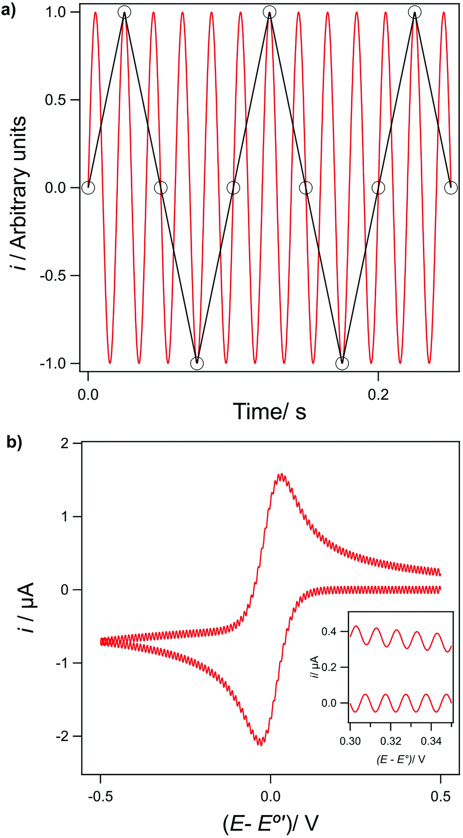 | ||
| Fig. 8 (a) A 50 Hz sine wave sampled at 4000 Hz (red), which gives high fidelity. The black trace shows the same 50 Hz sine wave sampled at 40 Hz at points marked with black open circles, which results in aliasing of the 50 Hz down to 10 Hz. (b) COMSOL simulated CV data sampled at 200 Hz. When a 210 Hz sine wave is added, the noise is aliased down to 10 Hz, as can be seen from the inset. | ||
In electrochemistry, low currents e.g. nA and smaller and high resistance (potentiometry) circuits are particularly susceptible to noise interference and even very modest electromagnetic coupling of noise can lead to spurious signals that swamp the signal being measured. The electrochemists often go-to tool to defeat such noise is the Faraday cage, an enclosure with a continuous covering of conductive material which effectively blocks the ingress of electromagnetic fields. The presence of holes in the Faraday cage are problematic as any electromagnetic radiation which has a wavelength less than double the longest dimension of the aperture is not attenuated by the cage and is likely to be rectified by instruments inside. This results in the detection of these signals as AC noise which often has a 50 Hz, 60 Hz or even 100 kHz fundamental. In theory a Faraday cage does not need to be connected to ground to block electromagnetic fields. However, as most practical cages require a door for access and wiring connections between the inside and outside of the cage, it must be grounded for operational and safety reasons in order to prevent electrical shock.
In most experimental situations the potentiostat sits outside the Faraday cage. Under these conditions the Faraday cage should be connected to the same ground point (common earth) as the potentiostat, using separate earth cables. This is referred to as “star earthing” and is true of all instrumentation which is used in conjunction with the electrochemical experiment but sits outside the Faraday cage. Instrumentation inside the grounded cage can be simply grounded to the cage itself. Most commercial potentiostats have a ground connector, usually a socket or threaded bolt to which a ground connection can be made. A chassis connector (chassis is the metal box of the potentiostat) is also common, which also should be grounded for both safety reasons and to protect the internal circuitry from noise.
The ideal ground connection is a certified local earthing rod (clean earth) buried in the ground (very dry ground is not good!) adjacent to the laboratory to which the external contacts e.g. Faraday cage, potentiostat can be made. Labs often have a hole drilled in the wall to make the external connection between the equipment and the rod. If your laboratory does not have this it is possible to run a separate earth wire back to the consumer unit i.e. local sub-station, but this could be impractical based on distance. If all else fails the mains earth of a power outlet will suffice i.e. connecting your potentiostat ground point to a specialty plug which only contains an earth pin, which is then plugged into a mains plug socket. However, this is likely to be noisier. If you are using this route, noise may be further reduced by plugging the potentiostat power cable first into an isolation transformer, and then plugging this transformer into the mains; the transformer acts to isolate the potentiostat from the mains supply. The potentiostat ground point must still be connected to a star earth point. Note, if the potentiostat is directly connected to the mains supply, laboratory equipment that intermittently draws significant current, such as an oven or hotplate, should definitely not be powered using the same branch circuit as the potentiostat. Whilst battery powered potentiostats will generate lower internal noise they are still sensitive to external noise.
Wires and cables demand special attention since in addition to electromagnetically coupled noise they may also carry internally generated noise from the instrumentation they are connected to outside of the cage. All wires and cables, wherever possible, should be electrically shielded from the instrument to the cage and again once inside the cage, from the entry point to as close as possible to the electrochemical cell. Shielded or screened cables are ones in which the conductive wire or wires are encased in insulator but contain a second conductive layer, on top of the insulating layer, usually in the form of a copper braid which acts as a mini Faraday cage. The wire which contains the two conducting layers is referred to as a co-axial cable. If possible cables carrying alternating high voltages such as mains should be avoided because the alternating high voltages radiate as noise inside the Faraday cage. Piezo-electric cables have a similar effect, which can be problematic for electrochemical researchers developing electrochemical scanning probe instruments, which will also be measuring small currents.
Any wire or other conductive object, such as “helping hands” entering the Faraday cage should be thought of as an antenna picking up electromagnetic noise from the outside environment and radiating it inside the cage. To minimize this effect, all conductive objects placed inside the cage should be grounded to the Faraday cage, which itself is grounded. For coaxial wires the outer conductive layer should be electrically coupled to the cage at the entry point. This is typically implemented in practice through the use of double-ended chassis mounted connectors directly incorporated into the cage or capacitively decoupling the wire at the point it enters the cage; a capacitor attached between the outer conductive layer of the wire and ground will conduct ac noise to ground. Keeping digital equipment, for example computers or mobile (cell) phones and their earth connections away from the cage is also always helpful. Desktop computers are also often sources of high frequency noise.
Fig. 9a shows an interesting example of noise pick-up under conditions where noise issues will be especially prevalent i.e. when measuring very small currents. In particular it highlights the problem of having a mobile (cell) phone too close to the experiment. Here a current of ∼90 pA is being recorded as a result of measuring the conductivity of an electrolyte-filled nanopipette.43 The current is measured using a HEKA EPC10 USB patch clamp amplifier, with the preamplifier (headstage) and nanopipette placed inside a home-built Faraday cage. The mobile phone produces a series of bursts of radio frequency “chirps” at variable intervals in the 2.5 GHz to 5 GHz region. Fig. 9b shows an expanded view of one burst and the effect it has on the signal. Each chirp of radio frequency is rectified by the amplifier to produce a step in voltage with additional spikes as the chirp starts and stops. A careless experimenter could leave their mobile phone on the lab bench next to this experiment and be totally oblivious to the potentially drastic effect it may be having on their results!
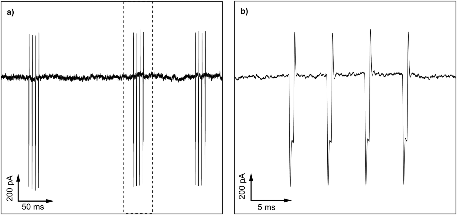 | ||
| Fig. 9 (a) Noise on the i–t signal for a glass nanopipette conductivity measurement recorded using a HEKA EPC10 USB Amplifier induced by a mobile phone, (b) zoomed in region, highlighted by the dotted line in (a). | ||
A useful guide to minimizing or ideally eliminating noise, including a noise troubleshooting table (Table 3) is included below. Practical guidelines on how to look for, measure and reduce noise experimentally are also given in SI 4 (ESI†). After reading the information in 1–9 below, Table 3 and SI 4 (ESI†), the researcher is encouraged to investigate for themselves the sources of noise in their set-up and to experiment with noise reduction strategies.
(1) Use a Faraday cage, this is essential for low current, high resistance measurements.
(2) Set your kit up away from obvious noise sources e.g. electric motors, switches, lifts (elevators), mobile (cell) phones.
(3) Use wires, where possible, that are electrically shielded and keep them short.
(4) Consider whether there is any advantage to using battery powered laptops and potentiostats.
(5) Ground the Faraday cage and potentiostat to the same earth “star earthing”.
(6) Use a good clean (low noise) earth connection.
(7) Switch Bluetooth and wireless off in any nearby device unless essential to operation.
(8) Minimize vibration.
(9) Allow the equipment to warm up and minimize temperature changes.
Only when noise sources have been correctly dealt with should filtering be employed, and this should be done with great care to avoid what can be undetectable and misleading distortion in the signals.
9. Filters
Once all possible precautions have been taken to minimize noise pick-up, the use of analogue electronic filters, applied during data collection and possibly also digital filters (applied using computer software post data collection) to further clean up the signal may still be required. The purpose of the filters are to reduce the amplitude or intensity of the noise in the signal without affecting important features of the signal such as time constant, peak potential, peak width etc. This is only possible if the signal and the noise have different frequencies. Typically the noise most commonly encountered on the CV response will be 50 Hz or 60 Hz from the power supply. Hence a filter needs to act like an amplifier where the gain is one for the frequencies of interest and ideally much less than one, for noise frequencies. The majority of commercial potentiostat instrumentation comes with various levels of analogue filters built in which the user may or may not be aware of.Potentiostat analogue filters
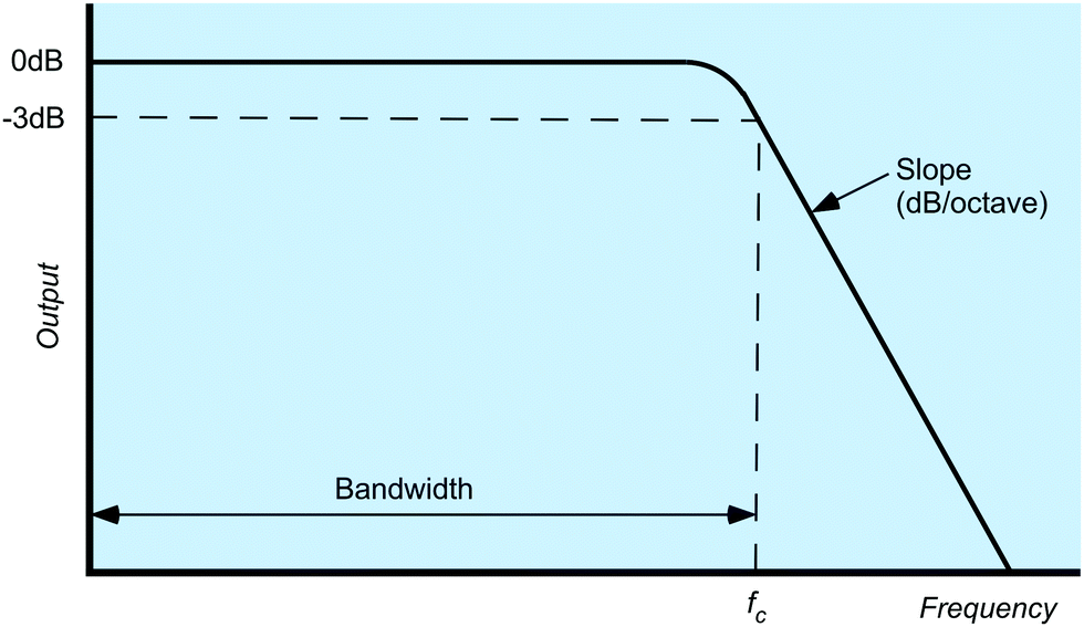
There are broadly four categories of electronic filter: (1) the low pass filter, the most common type of filter employed in electrochemical potentiostats, which attenuates higher frequencies and allows low frequencies to pass unhindered; noise is typically of a higher frequency than the desired signal. (2) The high pass filter which allows higher frequencies to pass but attenuates lower frequencies (3) the notch filter which blocks a specific frequency; and (4) a bandpass filter which allows all frequencies between two characteristic frequencies to pass. Given its importance the low pass filter is often a user-selected feature in the potentiostat software. Furthermore, analogue-to-digital conversion of the current (as a voltage) requires the use of a low pass filter to prevent signal fluctuations during the time it takes to convert the voltage to a digital number. All commercial potentiostats will therefore have both low pass filtering which cannot be switched off and optional additional user-selected low-pass filters.Fig. 10 shows, the frequency-output response of a low pass filter. The point at which frequencies start to be attenuated is called the “cut-off frequency” (fc) or “turnover point” and by convention is defined as the frequency when attenuation reaches −3 decibels (dB), where a dB is defined by eqn (12) for voltage signals:
| dB = 20log (signal voltage out/signal voltage in) | (12) |
 | ||
| Fig. 10 Frequency response of an analogue low pass filter. | ||
Proper application of electronic filters requires that the frequencies of all experimental signals fall within the bandwidth of the filter and all the frequencies of any undesirable signals fall as deeply as possible into the slope region of the filter to maximize attenuation. A fast Fourier transform (FFT) of the signal being measured is a valuable tool in working out the frequency of the noise (see FFT data in SI 4 and Fig. S5b, ESI†). Once the noise frequencies are known there are many on-line tools which enable you to calculate fc and order of the filter required to reduce the amplitude of a specific frequency signal by a defined amount. For example to reduce a 50 Hz signal by an order of magnitude a second order filter with fc of 5 Hz can be used. However, take care, if the signal also has characteristic components with frequencies of 5 Hz or more as this can lead to distortion of voltammetric peak shapes. For example, a voltammetric peak 100 mV wide, scanned at 0.5 V s−1 (=0.2 s) has an “effective” frequency of ca. 5 Hz. Furthermore, the peak itself will have sharp features which will have higher frequencies still. Such a peak would therefore be severely distorted with a low pass filter of fc = 5 Hz. To avoid distortions, it is best to eliminate this external noise in the first place or, in this case, scan more slowly.
Box 1: The basic electronic components (and symbols) the electrochemist should be familiar with. Definitions of Ohm's and Kirchoff's laws and voltage dividers
|
To further illustrate the point, Fig. 11 shows the effects of low pass filters on COMSOL simulated CV data (Fig. 6b, Ru = 0 Ω) to which 50 Hz sinusoidal noise (50 nA amplitude ca. 2.5% of the peak current) has been deliberately added via simulation (IgorPro). The COMSOL CV has 4000 data points and was recorded at 0.1 V s−1 (sampling frequency = 200 Hz). Fig. 11 shows the effects of using three different second order low pass filters with fc values of (b) 50 Hz; (c) 5 Hz and (d) 0.5 Hz. (a) is the unfiltered CV. With fc = 50 Hz, the filter barely attenuates the simulated 50 Hz noise, bringing the amplitude down to 35 nA. Decreasing fc to 5 Hz this filter almost completely removes the 50 Hz noise, reducing the noise amplitude by two orders of magnitude to 0.6 nA, but without unduly distorting the voltammogram; peak potentials and peak widths are essentially unaltered. The important characteristics of the CV fall within the bandwidth of the filter and pass through with unity gain. With fc = 0.5 Hz whilst the noise is effectively removed (dotted line) the CV is now distorted compared to the unfiltered CV (solid line) and the key important voltammetric parameters are all incorrectly represented: peak potential, peak width, peak height and peak separation.
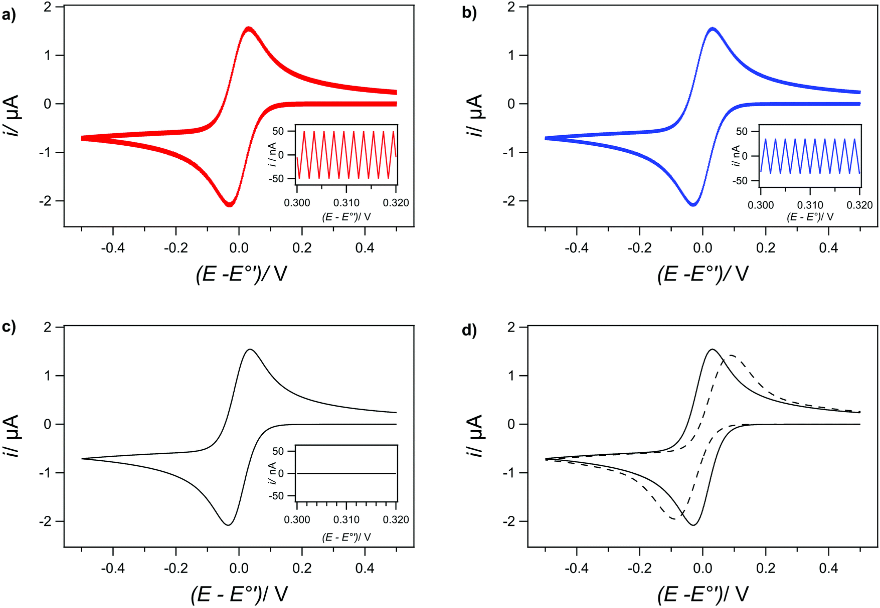 | ||
| Fig. 11 (a) 50 Hz, 50 nA amplitude noise added to a simulated CV data. The inset shows a zoom of the noise. Also shown is the same data after being passed through a digitally simulated second order filter with fc values of (b) 50 Hz; (c) 5 Hz and (d) 0.5 Hz (dotted line). The solid line shows the noise free original CV data for comparison. | ||
10. Conclusions
Having an appreciation of how a three electrode potentiostat works when recording a CV is incredibly beneficial to the electrochemist. This tutorial paper outlines the important op-amp components of the potentiostatic circuit, in particular (1) the control amplifier, which is used to keep the potential at the RE at a known value with respect to the WE, by adjusting the potential on the CE, and (2) the current follower, which converts the current flowing through the WE to an output voltage proportional to the current. We highlight the importance of understanding the resistances which exist in the potentiostatic circuit in particular RC–R and RR–W the former which is compensated for by the potentiostat and Ru (the component of RR–W) which remains uncompensated. Appreciating such concepts is crucial when making practical measurements and helps understand, for example: (i) why a RE should never be disconnected when the potentiostat is actively applying a potential; (ii) how poor electrode contacts, blocked RE frits, wet cables, electrodes touching the sides of the reaction vessel can all contribute to Ru resulting in distortion of the real data; (iii) the choice of CE electrode material and associated electron transfer reactions, CE size and separation from the RE, clean RE frits, are all important in maintaining a CE potential below the compliance voltage. We also highlight the limitations of laboratory based DVMs in measuring the true potential established at a glass pH probe and discuss the advantage of using voltage follower op-amp circuits in potentiometric measurements.An understanding of how the digital computer generates a data stream for the potentiostat DAC to convert into a voltage waveform and how the potentiostat outputs the experimental data via ADC is shown to be important. Knowledge of bit size which defines the resolution of the measurement is necessary when selecting an appropriate current sensitivity (or gain) setting. Given much of the original electrochemical theory was developed before the digital age using analogue techniques, an appreciation of the difference between recording an analogue CV versus a digital staircase CV is also highlighted. Practical methods for reducing or removing noise on the CV are also provided. Given all potentiostats use filters, in particular low pass filters, the basic concept of filters are discussed and in particular what happens to CV data when the wrong filter is employed.
Finally, whilst it is generally the case that mysterious or uninterpretable data usually arise as a result of the electrochemical cell being set up badly, potentiostat failures are regrettably not unknown. A dummy cell (often supplied with the potentiostat) is a useful check on instrument performance, typically consisting of two resistors and a capacitor. The first resistor reflects Ru, for example, for work in background electrolyte containing aqueous solutions, 10 Ω is a useful value. The second resistance should be selected to give a maximum current similar to the range expected from the electrochemical experiment. For example if currents ca. 10 μA are expected (at 1 V) then a 100 kΩ resistance is appropriate. The capacitor is often chosen to reflect Cdl. For Pt or Au electrodes, Cdl values are in the range 20–50 μF cm−2; a 2 mm diameter electrode would be represented by a capacitor of 0.6–1.5 μF. A CV recorded with such a dummy cell should show a slope consistent with Ohm's law (1/Ru) and a hysteresis consistent with Cdl.
Author contributions
Alex W. Colburn performed, conceptualisation, writing-original draft, writing – review and visualisation. Katherine J. Levey performed, investigation, formal analysis, writing – review and visualisation. Danny O’Hare performed formal analysis, writing – review and visualisation. Julie V. Macpherson performed, conceptualisation, writing-original draft, writing – review and editing, supervision and project administration.Conflicts of interest
There are no conflicts to declare.Acknowledgements
This article is one that the authors have been wanting to write for a significant period of time. The first UK lock-down period of COVID-19 provided the opportunity to finally commence. We acknowledge the Centre for Doctoral Training in Diamond Science and Technology (EP/L015315/1) for funding for KJL. We thank Dr Martin Andrew Edwards (Department of Chemistry, University of Arkansas, US) for providing the data for Fig. 9 and Mr James Colburn for designing the TOC image. We thank Dr Gabriel Meloni and the following members of the Macpherson and O’Hare research groups for their helpful discussion of the paper and various potentiostat related issues they have encountered over the years: Irina Terrero Rodríguez, Sophie Webb, Zhaoyan Zhang, Daniel Houghton, Georgia Wood, Emily Braxton, Nicole Reily, Joshua Tully, Teena Rajan, Dana Druka, Dr Sally Gowers, Dr Dave Freeman, James Mcleod, Saylee Jangam, Dr Isobel Steer, Nathanael Tan.References
- A. A. Belyustin, J. Solid State Electrochem., 2011, 15, 47–65 CrossRef CAS.
- A. J. Bard and L. R. Faulkner, Electrochemical Methods: Fundamentals and Applications, Wiley, New York, 2nd edn, 2000 Search PubMed.
- S. W. Boettcher, S. Z. Oener, M. C. Lonergan, Y. Surendranath, S. Ardo, C. Brozek and P. A. Kempler, ACS Energy Lett., 2021, 6, 261–266 CrossRef CAS.
- H. Kahlert, in Electroanalytical Methods, ed. F. Scholz, Springer Berlin Heidelberg, Berlin, Heidelberg, 2005, pp. 261–278 Search PubMed.
- A. W. Bott, Curr. Sep., 1995, 14, 64–68 CAS.
- J. J. Fritz, J. Solut. Chem., 1985, 14, 865–879 CrossRef CAS.
- R. P. Buck, S. Rondinini, A. K. Covington, F. G. K. Baucke, C. M. A. Brett, M. F. Camões, M. J. T. Milton, T. Mussini, R. Naumann, K. W. Pratt, P. Spitzer and G. S. Wilson, Pure Appl. Chem., 2003, 74, 2169–2200 Search PubMed.
- K. Diem and C. Lentner, Scientific Tables, Ciba-Geigy Limited, 7th edn, 1970, pp. 653–654 Search PubMed.
- A. Hickling, Trans. Faraday Soc., 1942, 38, 27–33 RSC.
- G. N. Meloni, J. Chem. Educ., 2016, 93, 1320–1322 CrossRef CAS.
- M. W. Glasscott, M. D. Verber, J. R. Hall, A. D. Pendergast, C. J. McKinney and J. E. Dick, J. Chem. Educ., 2020, 97, 265–270 CrossRef CAS.
- A. A. Rowe, A. J. Bonham, R. J. White, M. P. Zimmer, R. J. Yadgar, T. M. Hobza, J. W. Honea, I. Ben-Yaacov and K. W. Plaxco, PLoS One, 2011, 6, e23783 CrossRef CAS PubMed.
- P. Horowitz and W. Hill, The Art of Electronics, Cambridge University Press, 3rd edn, 2015 Search PubMed.
- P. T. Kerridge, Biochem. J., 1925, 19, 611–617 CrossRef CAS PubMed.
- D. Woermann, Ber. Bunseng. Phys. Chem., 1973, 77, 737 Search PubMed.
- H. Jin, Y. Qin, S. Pan, A. U. Alam, S. Dong, R. Ghosh and M. J. Deen, J. Chem. Educ., 2018, 95, 326–330 CrossRef CAS.
- S. C. Costa and J. C. B. Fernandes, J. Chem. Educ., 2019, 96, 372–376 CrossRef CAS.
- J. C. Myland and K. B. Oldham, Anal. Chem., 2000, 72, 3972–3980 CrossRef CAS PubMed.
- T. J. Smith and K. J. Stevenson, in Handbook of Electrochemistry, ed. C. G. Zoski, Elsevier, 2007, pp. 73–110 Search PubMed.
- B. Ilic, D. Czaplewski, P. Neuzil, T. Stanczyk, J. Blough and G. J. Maclay, J. Mater. Sci., 2000, 35, 3447–3457 CrossRef CAS.
- J. V. Macpherson, Phys. Chem. Chem. Phys., 2015, 17, 2935–2949 RSC.
- A. Verdaguer-Casadevall, D. Deiana, M. Karamad, S. Siahrostami, P. Malacrida, T. W. Hansen, J. Rossmeisl, I. Chorkendorff and I. E. L. Stephens, Nano Lett., 2014, 14, 1603–1608 CrossRef CAS PubMed.
- D. S. P. Cardoso, B. Šljukić, D. M. F. Santos and C. A. C. Sequeira, Org. Process Res. Dev., 2017, 21, 1213–1226 CrossRef CAS.
- I. Hickman, Analog Circuits Cookbook, Elsevier, 2nd edn, 1999, pp. 653–654 Search PubMed.
- P. T. Kissinger and W. R. Heineman, eds., Laboratory Techniques in Electroanalytical Chemistry, CRC Press, 2nd edn, 1996 Search PubMed.
- P. He and L. R. Faulkner, Anal. Chem., 1986, 58, 517–523 CrossRef CAS.
- M. P. S. Mousavi, S. A. Saba, E. L. Anderson, M. A. Hillmyer and P. Bühlmann, Anal. Chem., 2016, 88, 8706–8713 CrossRef CAS PubMed.
- N. N. Elgrishi, K. J. Rountree, B. D. Mccarthy, E. S. Rountree, T. T. Eisenhart and J. L. Dempsey, J. Chem. Educ., 2018, 95, 197–206 Search PubMed.
- R. S. Nicholson and I. Shain, Anal. Chem., 1964, 36, 706–723 CrossRef CAS.
- S. J. Cobb and J. V. Macpherson, Anal. Chem., 2019, 91, 7935–7942 CrossRef CAS PubMed.
- M. E. Orazem and B. Tribollet, Electrochemical Impedance Spectroscopy, John Wiley & Sons, Inc., Hoboken, NJ, USA, 2017 Search PubMed.
- J. T. Cox and B. Zhang, Annu. Rev. Anal. Chem., 2012, 5, 253–272 CrossRef CAS PubMed.
- R. J. Forster, Chem. Soc. Rev., 1994, 23, 289–297 RSC.
- R. Bilewicz, R. A. Osteryoung and J. Osteryoung, Anal. Chem., 1986, 58, 2761–2765 CrossRef CAS.
- C. Batchelor-McAuley, M. Yang, E. M. Hall and R. G. Compton, J. Electroanal. Chem., 2015, 758, 1–6 CrossRef CAS.
- A. Bott, Curr. Sep., 1997, 1, 23–26 Search PubMed.
- B. Hai, Y. V. Tolmachev, K. A. Loparo, C. Zanelli and D. Scherson, J. Electrochem. Soc., 2011, 158, F15 CrossRef CAS.
- Z. Stojek and J. Osteryoung, Anal. Chem., 1991, 63, 839–841 CrossRef CAS.
- H. A. Heering, M. S. Mondal and F. A. Armstrong, Anal. Chem., 1999, 71, 174–182 CrossRef CAS PubMed.
- C. Montella, J. Electroanal. Chem., 2018, 817, 73–88 CrossRef CAS.
- J. Harberts, M. Kusch, J. O’Sullivan, R. Zierold and R. H. Blick, Bioengineering, 2020, 7, 46 Search PubMed.
- S. Fletcher, Fletcher S. Digital Sampling Strategies that Discriminate Against Mains Interference (Noise). A Tutorial Review. In: Microelectrodes: Theory and Applications. NATO ASI Series (Series E: Applied Sciences), Springer, Dordrecht, 1991 Search PubMed.
- M. A. Edwards, S. R. German, J. E. Dick, A. J. Bard and H. S. White, ACS Nano, 2015, 9, 12274–12282 CrossRef CAS PubMed.
Footnote |
| † Electronic supplementary information (ESI) available: SI 1 – estimating the maximum current that should be passed in a two-electrode system, SI 2 – finite element modelling of cyclic voltammetry incorporating Ohmic drop, SI 3 – electronic circuit for a two electrode set-up and SI 4 – probing and minimizing noise (PDF). COMSOL-generated report corresponding to the finite element model described in SI-2 (PDF). See DOI: 10.1039/d1cp00661d |
| This journal is © the Owner Societies 2021 |