Evaluation of nine condensed-phase force fields of the GROMOS, CHARMM, OPLS, AMBER, and OpenFF families against experimental cross-solvation free energies

Abstract

Experimental solvation free energies are nowadays commonly included as target properties in the validation of condensed-phase force fields, sometimes even in their calibration. In a previous article [Kashefolgheta et al., J. Chem. Theory. Comput., 2020, 16, 7556–7580], we showed how the involved comparison between experimental and simulation results could be made more systematic by considering a full matrix of cross-solvation free energies . For a set of N molecules that are all in the liquid state under ambient conditions, such a matrix encompasses N × N entries for considering each of the N molecules either as solute (A) or as solvent (B). In the quoted study, a cross-solvation matrix of 25 × 25 experimental value was introduced, considering 25 small molecules representative for alkanes, chloroalkanes, ethers, ketones, esters, alcohols, amines, and amides. This experimental data was used to compare the relative accuracies of four popular condensed-phase force fields, namely GROMOS-2016H66, OPLS-AA, AMBER-GAFF, and CHARMM-CGenFF. In the present work, the comparison is extended to five additional force fields, namely GROMOS-54A7, GROMOS-ATB, OPLS-LBCC, AMBER-GAFF2, and OpenFF. Considering these nine force fields, the correlation coefficients between experimental values and simulation results range from 0.76 to 0.88, the root-mean-square errors (RMSEs) from 2.9 to 4.8 kJ mol⁻¹, and average errors (AVEEs) from −1.5 to +1.0 kJ mol⁻¹. In terms of RMSEs, GROMOS-2016H66 and OPLS-AA present the best accuracy (2.9 kJ mol⁻¹), followed by OPLS-LBCC, AMBER-GAFF2, AMBER-GAFF, and OpenFF (3.3 to 3.6 kJ mol⁻¹), and then by GROMOS-54A7, CHARM-CGenFF, and GROMOS-ATB (4.0 to 4.8 kJ mol⁻¹). These differences are statistically significant but not very pronounced, and are distributed rather heterogeneously over the set of compounds within the different force fields.

---

1 Introduction

The comparison between simulation results and experimental values for the hydration free energies of small organic molecules has become a key component in the validation,^1–12 sensitivity assessment,^13–16 fine tuning,^{6,8,15,17–25} and even calibration^26–32 of condensed-phase force fields. Sometimes, solvation free energies in lower-polarity solvents (e.g. octanol, chloroform, cyclohexane, or hexane) are considered as well, and the corresponding experimental values (or the related transfer free energies from water) are also included in force-field validation^33–37 or calibration.^{25,28–30,32} In a few cases, more extensive sets of solute–solvent pairs have also been considered.^{10,11,38–42} However, in all the above situations, the selection of the systems included in the comparison is mainly based on the availability of experimental data, and the resulting sets may be rather imbalanced in terms of the intermolecular interactions they probe.

In a recent article,⁴³ we reported on an attempt to make this approach more systematic, by introducing a full matrix of standard Gibbs cross-solvation free energies . For a set of N molecules that are all in the liquid state under ambient conditions, such a matrix encompasses N × N entries for considering each of the N molecules either as solute (A) or as solvent (B). The point-to-point or Ben–Naim standard-state convention^44–46 was adopted, which implies that the same reference molar volumes are employed for the ideal-gas and the ideal-solution states. In this convention, corresponds to the reversible work for transferring one molecule of A from a fixed point in vacuum (infinitesimal-pressure limit) to a fixed point in the bulk of the solvent B (infinite-dilution limit), expressed on a per-mole basis. The transfer is performed at a constant temperature T⁻ = 298.15 K (both phases) and at a constant pressure P^o = 1 bar (solution phase). Note that these cross-solvation free energies include the self-solvation free energies as special cases, along the diagonal of the matrix.

A set of N = 25 organic molecules were considered, shown in Fig. 1 along with the acronyms used to refer to them in the article (see also Table 1 in ref. 43 for key properties of these compounds). These molecules involve one to seven carbon atoms and are representative for alkanes, chloroalkanes, ethers, ketones, esters, alcohols, amines, and amides. The set is divided into three categories based on the molecule polarity (as estimated by its molecular dipole moment), namely low-polarity (LP), medium-polarity (MP), or high-polarity (HP). Based on seven experimental data sources,^47–53 and after careful data curation (see Appendix A in ref. 43), a complete matrix of 625 entries was constructed, which is shown in Fig. 2a along with standard deviations σ over the available experimental estimates in Fig. 2b (see Table S1 in ref. 43 for the numerical values; the corresponding data files, labelled version 1.1, are also freely downloadable from the net under ref. 54).

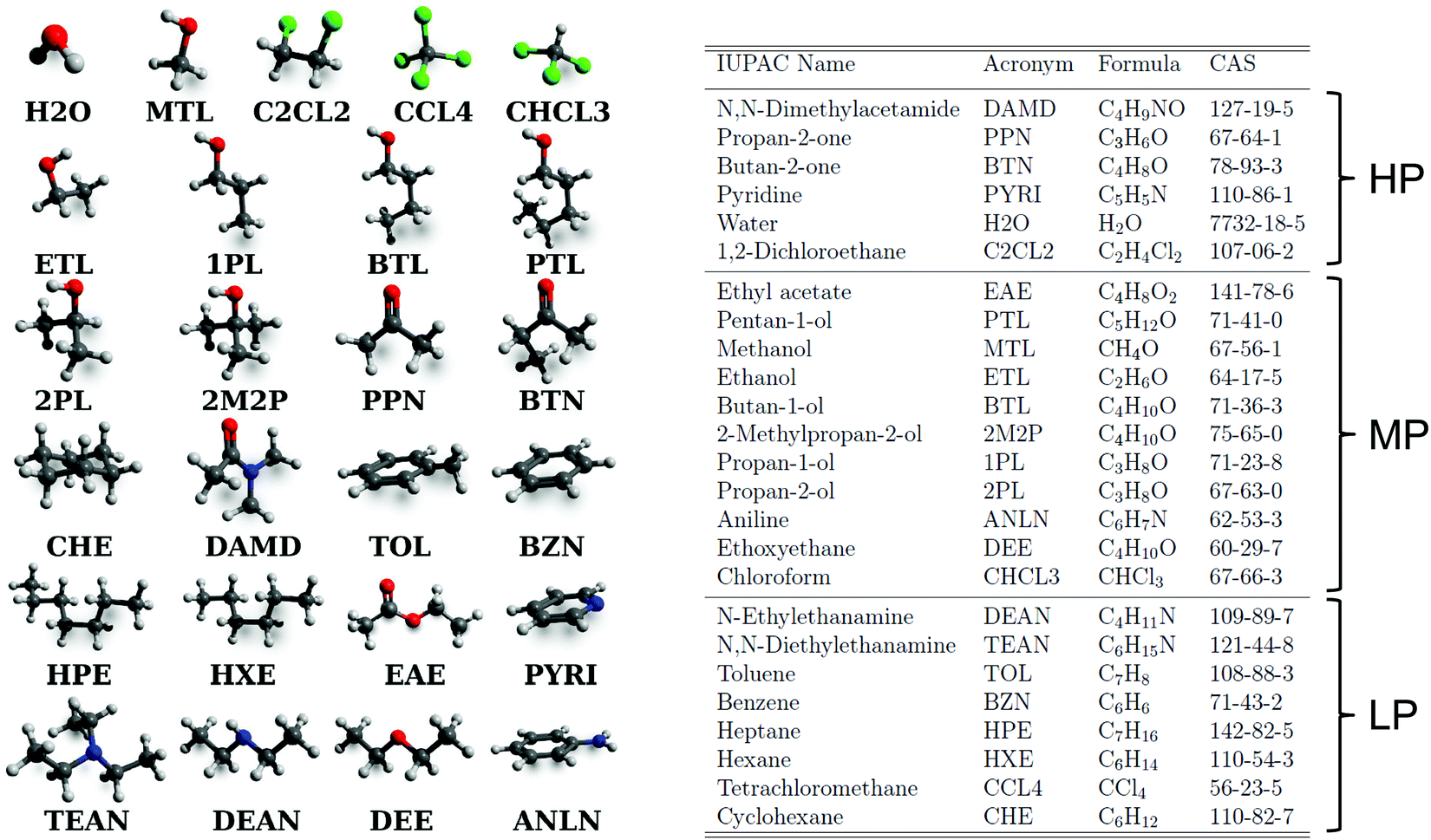Fig. 1 Molecular structures, acronyms, and identifiers of the 25 organic molecules considered in this work. The three- to five-letter acronyms are used to refer to each molecule in the text. For water, the acronym H₂O is sometimes replaced by the specification of a water model, namely the simple point charge water model¹¹⁶ (SPC) or the three-point transferable intermolecular potential TIP3P model^117,118 (TP3). The identifiers are the International Union of Pure and Applied Chemistry (IUPAC) name and the Chemical Abstract Service (CAS) registry number. Some key experimental properties (molecular dipole moment μ; melting temperature T_m, and boiling temperature T_b at 1 bar; liquid density ρ_liq, vaporization enthalpy ΔH_vap, and static relative dielectric permittivity ε at 298.15 K and 1 bar) can be found in Table 1 of ref. 43. The molecules are listed in order of decreasing polarity, as estimated by μ, and assigned to three categories of polarities, labelled high (HP), medium (MP), or low (LP) polarity.

Fig. 2 Recommended experimental values (a) for the cross-solvation free energies of 25 solutes A (rows) in the same 25 solvents B (columns), and associated standard deviations σ (b) over available experimental estimates (the gray pixels indicate 176 values that only occur once in the experimental references considered). The molecules considered and their acronyms are shown in Fig. 1. They are listed along the rows and columns in order of decreasing polarity, as estimated by the molecular dipole moment μ, and the partitioning into low (LP), medium (MP), and high (HP) polarity categories also indicated. The corresponding numerical data can be found in Table S1 of ref. 43. The corresponding data files, labelled version 1.1, are also freely downloadable from the net under ref. 54.

In the previous article,⁴³ this matrix of experimental values was used to compare the relative accuracies of four popular condensed-phase force fields, namely GROMOS-2016H66 (ref. 32), CHARMM-CGenFF (ref. 55 and 56), OPLS-AA (ref. 57–64), and AMBER-GAFF (ref. 65 and 66). In broad terms, and in spite of very different functional-form choices and parametrization strategies, the four force fields were found to perform similarly well. Relative to the experimental values, the root-mean-square errors (RMSEs) ranged between 2.9 and 4.0 kJ mol⁻¹ (lowest value of 2.9 for GROMOS-2016H66 and OPLS-AA), and the average errors (AVEEs) ranged between −0.8 and +1.0 kJ mol⁻¹ (lowest magnitude of 0.2 for CHARMM-CGenFF and AMBER-GAFF). These differences are statistically significant but not very pronounced, especially considering the influence of outliers, some of which possibly caused by inaccurate experimental data.

In the present study, we extend the comparison to five additional parameter sets, namely GROMOS-54A7 (ref. 27), GROMOS-ATB (ref. 36 and 67), OPLS-LBCC (ref. 57, 58 and 68; the OPLS-AA force field^57–64 with 1.14 × CM1A-LBCC charges⁶⁸), AMBER-GAFF2 (ref. 66 and 69; GAFF2 as distributed within the Antechamber package⁷⁰ in AmberTools16;⁷¹ see also ref. 37 and 72–75 for recent validation work), and OpenFF (ref. 72, 76 and 77; also accessible under ref. 78). The three GROMOS sets rely on a united-atom representation of the aliphatic groups, whereas all the other sets correspond to all-atom force fields.

2 Methods

2.1 Force fields

The nine force fields under comparison are listed in Table 1, along with a summary of their main differences in terms of design and parametrization. These differences are briefly explicited in the following paragraphs.

Table 1 The nine force fields compared in this work, along with a summary of their main differences in terms of design and parametrization. The force-field specification includes the family (Fam.), the specific parameter set (Set), whether the force field is all-atom (AA; as opposed to united-atom for the aliphatic groups), and whether the force field is newly considered in this article (New; as opposed to already considered in ref. 43). The treatment of the electrostatic interactions includes the method (EL Meth.), the derivation scheme for the atomic partial charges (Charge Deriv.), and the adjustment of the third-neighbor electrostatic interactions (3rd Nei. EL). The treatment of the Lennard-Jones interactions includes the method (LJ Meth.), the type of combination rules (Comb. Rules), and the adjustment of the third-neighbor Lennard-Jones interactions (3rd Nei. LJ). The standard water model (H₂O) is indicated, namely the simple point charge water model¹¹⁶ (SPC) or the three-point transferable intermolecular potential TIP3P model^117,118 (TP3). For each force field, this model is the only one considered in the present simulations (see ref. 43 for results corresponding to CHARMM-CGenFF, OPLS-AA, and AMBER-GAFF along with the SPC model). Note that the CHARMM-CGenFF simulations actually rely on a slightly modified mTIP3P model,¹²² involving non-zero Lennard-Jones interaction parameters on the hydrogen atoms (for simplicity, the same acronym TP3 is still used to refer to this model). In GROMOS-2016H66 and GROMOS-54A7, the models for CHCL3 and CCL4 are taken from ref. 115 and 123, respectively. The model for C2CL2 in GROMOS-2016H66 is taken from ref. 124. The OPLS model for CHCL3 is taken from ref. 125. Molecules that could not be simulated are also indicated (NS). This occurs when a corresponding model is unavailable in the given parameter set. The resulting numbers of molecule pairs in the FULL set (N_FULL), in the COMP set (N_COMP), and in the CONF set (N_CONF) are also indicated. Abbreviations: SMIRNOFF-99Frosst v1.0 (S99F1.0), reaction-field (RF), particle-mesh Ewald (PME), experiment (Exp.), quantum mechanics (QM), correction (Corr.), potential (Pot.), switch (Swi.), special (Spec.)

Fam.	Set	AA	New	EL Meth.	Charge Deriv.	3rd Nei. EL	LJ Meth.	Comb. Rules	3rd Nei. LJ	H2O	NS	N FULL	N COMP	N CONF
GROMOS	2016H66	—	—	RF 1.4 nm	Fit to exp.	Normal	Cutoff 1.4 nm	Geometric Mean	Spec. Set	SPC	—	25 × 25	22 × 22 − 2	340
							No Corr.
GROMOS	54A7	—	×	RF 1.4 nm	Fit to exp.	Normal	Cutoff 1.4 nm	Geometric Mean	Spec. Set	SPC	C2CL2	22 × 22	20 × 20 − 1	300
							No Corr.				DAMD, PYRI
GROMOS	ATB	—	×	RF 1.4 nm	Fit to QM	Normal	Cutoff 1.4 nm	Geometric Mean	Spec. Set	SPC	—	25 × 25	22 × 22 − 2	340
							No Corr.
CHARMM	CGenFF	×	—	PME	Fit to QM	Normal	Cutoff 1.2 nm +	Lorentz-Berthelot	Spec. Set	TP3	CHCL3,	23 × 23	22 × 22 − 2	340
							Tail Corr. + Force Swi. 0.2 nm				CCL4
OPLS	AA	×	—	PME	Fit to exp.	×0.5	Cutoff 1.1 nm +	Geometric Mean	×0.5	TP3	—	25 × 25	22 × 22 − 2	340
							Tail Corr. + Pot. Swi. 0.05 nm
OPLS	LBCC	×	×	PME	Fit to QM	×0.5	Cutoff 1.0 nm + Tail Corr. + Pot. Swi. 0.05 nm	Geometric Mean	×0.5	TP3	CCL4	24 × 24	22 × 22 − 2	340
AMBER	GAFF	×	—	PME	Fit to QM	×0.833	Cutoff 1.1 nm + Tail Corr. + Pot. Swi. 0.1 nm	Lorentz–Berthelot	×0.5	TP3	—	25 × 25	22 × 22 − 2	340
AMBER	GAFF2	×	×	PME	Fit to QM	×0.833	Cutoff 1.1 nm + Tail Corr. + Pot. Swi. 0.1 nm	Lorentz–Berthelot	×0.5	TP3	—	25 × 25	22 × 22 − 2	340
OpenFF	S99F1.0	×	×	PME	Fit to QM	×0.833	Cutoff 1.1 nm + Tail Corr. + Pot. Swi. 0.1 nm	Lorentz–Berthelot	×0.5	TP3	—	25 × 25	22 × 22 − 2	340

---

Except for GROMOS, all the force fields under comparison rely on a lattice-sum representation of the electrostatic interactions based on the particle-mesh Ewald^79,80 (PME) algorithm. In contrast, GROMOS uses a charge-group cutoff of 1.4 nm along with a reaction-field^81–84 (RF) approximation for the omitted electrostatic interactions beyond this distance.

The atomic partial charges in GROMOS-2016H66, GROMOS-54A7 and OPLS-AA are derived by optimization against experimental pure-liquid properties (and, possibly, solvation free energies) considering small organic molecules. In GROMOS-ATB, the charges are fitted to reproduce the quantum-mechanical (QM) electrostatic potential (ESP) using the Merz–Kollman (MK) scheme,^85,86 based on structures optimized at the B3LYP level of theory^87–90 with a 6-31G* basis set⁹¹ and a polarizable continuum model⁹² (PCM) for implicit solvation. The charges of chemically equivalent atoms are subsequently equalized.³⁶ In CHARMM-CGenFF, initial values for the charges are estimated either by analogy with similar groups in the CHARMM force field, or based on calculations at the second-order Møller–Plesser (MP2) level of theory⁹³ with a 6-31G(d) basis set⁹¹ and the MK scheme.^85,86 They are then further optimized to reproduce the QM gas-phase dipole moment and the interaction energy with a water molecule in different positions and orientations.^55,56 In OPLS-LBCC, the charges correspond to 1.14 × CM1A-LBCC charges, i.e. CM1A charges⁹⁴ amplified by an empirical factor^95,96 of 1.14 and further adjusted by localized bond-charge corrections⁶⁸ (BCCs). The CM1A charges are themselves derived following an empirical scheme⁹⁴ based on a Mulliken population analysis⁹⁷ of the electron density calculated at the AM1 semi-empirical level.⁹⁸ In AMBER-GAFF and AMBER-GAFF2, the charges are calculated using the restricted ESP (RESP) fitting protocol,⁹⁹ based on structures optimized at the Hartree–Fock (HF) level of theory^100,101 with a 6-31G(d) basis set⁹¹ in vacuum. Finally, in OpenFF, AM1-BCC charges^102,103 are used. These are derived from a Mulliken population analysis⁹⁷ performed at the AM1 level⁹⁸ by application of BCCs, with the goal of approximating HF/6-31G* RESP charges.

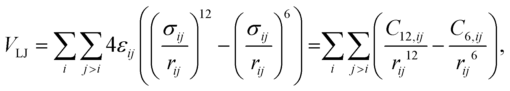
All the force fields under comparison are based on the same description of the van der Waals interactions relying on the Lennard-Jones function¹⁰⁴

where r_ij is the distance between atoms i and j, σ_ij the collision diameter, ε_ij the well depth, C_12,ij the repulsive coefficient, and C_6,ij the dispersive coefficient. The summation in this equation is restricted to pairs within the cutoff distance, which is set to 1.4 nm for GROMOS, 1.2 nm for CHARMM, 1.1 nm for OPLS-AA, AMBER and OpenFF, or 1.0 nm for OPLS-LBCC. For CHARMM, a Lennard-Jones force switch is applied over the last 0.2 nm. For OPLS, a Lennard-Jones potential switch is applied over the last 0.05 nm, while AMBER and OpenFF apply such a switch over the last 0.1 nm. The inclusion of long-range Lennard-Jones interactions (tail correction¹⁰⁵ or use of lattice summation^{13,80,106–110}) is inconsistent with the calibration of the GROMOS force fields.¹⁶ However, for CHARMM, OPLS, AMBER and OpenFF, a tail correction¹⁰⁵ is applied here in the calculation of the energy and virial.

The CHARMM, AMBER and OpenFF force fields rely on a strict Lorentz–Berthelot combination rule^111,112 for the Lennard-Jones interaction parameters. In contrast, the GROMOS and OPLS force fields rely on a geometric-mean combination rule.^113,114 For GROMOS, the application of this rule admits two exceptions. First, the repulsive coefficients C_12,ii and C_12,jj used to define C_12,ij can be taken from three alternative sets based on the types of the involved atoms, depending whether they are non-hydrogen-bonding (type I), uncharged hydrogen-bonding (type II), or oppositely charged (type III, for the negative species only). Only types I and II are relevant for the neutral molecules considered here. The second exception is that pair-specific parameter are used for the GROMOS-2016H66 and GROMOS-54A7 CHCL3 model.¹¹⁵

For all the force fields considered, first and second covalent neighbors are excluded from any non-bonded interaction. In GROMOS and CHARMM, the electrostatic interaction between third covalent neighbors is unaltered, and the Lennard-Jones interaction is defined based on a special set of third-neighbor parameters. For OPLS, both the electrostatic and the Lennard-Jones interactions are scaled by a factor of 0.5 for third neighbors. For AMBER and OpenFF, the electrostatic and Lennard-Jones interactions involving third neighbors are scaled by factors of 0.833 and 0.5, respectively.

Note that the Lennard-Jones interaction parameters of OpenFF relevant for the molecules considered here are in large part imported from AMBER-GAFF, so that the main difference between the two force fields resides in the covalent interaction parameters and the charge-derivation procedure. Similarly, since AMBER-GAFF and AMBER-GAFF2 have the same atomic partial charges, the only difference between the two force fields resides in the covalent and Lennard-Jones interactions parameters that were reoptimized for AMBER-GAFF2.

For each of the nine force fields, the compatible water model as well as a small subset of organic molecules possibly omitted from the simulations are also indicated in Table 1. The GROMOS force field is compatible with the simple point charge (SPC) water model.¹¹⁶ All the other force fields rely on the three-point transferable intermolecular potential (TIP3P) model,^117,118 further labelled TP3. This model is also adopted as a usual choice for OPLS-AA, although the force field was originally parametrized using the four-site TIP4P water model^117,118 instead^61,119,120 (unlike OPLS-LBCC, which directly¹²¹ relied on TIP3P). Note also that the CHARMM simulations actually rely on a slightly modified mTIP3P water model,¹²² involving non-zero Lennard-Jones interaction parameters on the hydrogen atoms. For simplicity, the same acronym TP3 is used to refer to this model as well. For each force field, the compatible water model is the only one considered in the present simulations (see ref. 43 for results using CHARMM-CGenFF, OPLS-AA, and AMBER-GAFF along with the SPC water model).

In GROMOS-2016H66 and GROMOS-54A7, the models for CHCL3 and CCL4 are taken from ref. 115 and 123, respectively. The model for C2CL2 in GROMOS-2016H66 is taken from ref. 124 (see ref. 43 for results with alternative CHCL3 and CCl4 models from ref. 124). The OPLS model for CHCL3 is taken from ref. 125. The simulations involving DAMD, PYRI and C2CL2 are not performed with GROMOS-54A7, as this set does not encompass building blocks for these molecules. Similarly, the simulations involving CHCL3 and CCL4 with CHARMM-CGenFF are omitted, as the corresponding parameters could not be obtained from the CHARMM-GUI server.^126–129 The same applies to CCL4 in OPLS-LBCC, where the parameters could not be derived using the LigParGen server.¹²¹ For each of the nine force fields, the resulting number N_FULL of calculated entries in the cross-solvation matrix are also reported in Table 1.

2.2 Simulation protocols

For GROMOS-2016H66, the topology building blocks³² for the molecules considered were taken directly from the GROMOS-2016H66 distribution.¹³⁰ For GROMOS-54A7, they were also obtained as topology building blocks²⁷ from the same site¹³⁰ (files used in ref. 32 for comparison between 2016H66 and 53A6, identical to 54A7 for these molecules). For GROMOS-ATB, the molecular topologies^36,67 were generated using the ATB server¹³¹ (version 3.0; the united-atom variant was selected). For CHARMM, the topologies were obtained from the CHARMM-GUI server.^126–129 For OPLS-AA, the topology files in GROMACS format were generated using the TPPMKTOP tool,¹³² and used together with the other OPLS parameters in the GROMACS distribution^133,134 (version 5.0.2). For OPLS-LBCC, the molecular topologies^57,58,68 were generated using the LigParGen server.¹²¹ For AMBER-GAFF2, the atomic partial charges were derived using the Antechamber⁷⁰ software package based on QM calculations relying on the Gaussian09 software.¹³⁵ Finally, for OpenFF, the molecular topologies were generated with the OpenForceField toolkit⁷² (version 0.5.0), using the rdkit software¹³⁶ for chemical perception and the force-field parameters from SMIRNOFF99Frosst (version 1.0.0), along with the partial charges obtained using Antechamber.⁷⁰

All simulations involved a single solute molecule in a cubic computational box containing 512 solvent molecules, except for the solvent water (1000 molecules). They were performed under periodic boundary conditions in the isothermal–isobaric (NPT) ensemble at P^o = 1 bar and T⁻ = 298.15 K. The temperature was maintained close to T⁻ by application of stochastic dynamics (SD) with a friction coefficient set to 10 ps⁻¹, except for the solvent water with GROMOS (91 ps⁻¹). The pressure was maintained close to P^o by application of a weak-coupling barostat¹³⁷ with a coupling time of 1 ps and an isothermal compressibility of 4.5 × 10⁻⁵ bar⁻¹, except for GROMOS (0.5 ps and 4.575 × 10⁻⁴ kJ mol⁻¹ nm³). The Langevin equation of motion was integrated using the leap-frog algorithm¹³⁸ (SD variant¹³⁹) with a timestep of 2 fs. The initial solute–solvent configurations were generated using the Packmol software,¹⁴⁰ and equilibrated at P^o and T⁻ during 0.2 ns, resulting in box edges ranging between 3.1 and 5.0 nm.

To calculate the solvation free energy, the solute–solvent Lennard-Jones and electrostatic interactions were gradually turned off in the Hamiltonian according to a coupling parameter λ, changing from zero (fully coupled) to one (fully decoupled). Note that the use of SD alleviates possible issues related to the lack of kinetic-energy exchange between solute and solvent close to the decoupled state. All calculations relied on simulations at fixed successive λ-values, each involving a sampling time of 3 ns after at least 0.1 ns equilibration.

For the GROMOS force field, these free-energy calculations were performed using the GROMOS software.^141–144 They relied on thermodynamic integration¹⁴⁵ with Simpson quadrature^146–148 (Kepler's wine barrel method¹⁴⁹) considering 21 equispaced λ-points. The solute–solvent electrostatic and Lennard-Jones interactions were decoupled simultaneously using a soft-core scheme¹⁵⁰ with the parameters α_LJ = 0.5 and α_C = 0.5 nm². The electrostatic interactions were calculated using a twin-range cutoff approach¹⁵¹ with short- and long-range cutoff distances set to 0.8 and 1.4 nm, respectively, and a frequency of 5 timesteps for the update of the short-range pairlist and intermediate-range interactions. A RF correction^81–84 was applied to account for the mean effect of the omitted electrostatic interactions beyond the long-range cutoff distance, using the permittivities listed in Table 1 of ref. 43, which correspond to experimental values except for water (permittivity of the SPC model). No correction was used for the corresponding long-range Lennard-Jones interactions. The SHAKE algorithm¹⁵² was applied to constrain all bond-lengths with a relative geometric tolerance of 10⁻⁴. For water (in all three GROMOS variants), as well as CHCL3 and CCL4 (in GROMOS-2016H66 and GROMOS-54A7), distance constraints were applied as well to keep the bond-angles rigid. The bond-angles in all the other molecules considered were treated as flexible. Note that GROMOS-2016H66 and GROMOS-54A7 rely on pair-specific Lennard-Jones interaction parameters for the GROMOS CHCL3 model.¹¹⁵ The center of mass translation of the computational box was removed every 2 ps. In a separate set of calculations, the electrostatic component ΔG_ELE of the solvation free energy was calculated by turning off only the electrostatic solute–solvent interactions, using a linear coupling scheme and 21 equispaced λ-points. The Lennard-Jones component ΔG_VDW was then deduced by subtracting ΔG_ELE from the total solvation free energy.

For CHARMM, OPLS, AMBER, and OpenFF, the free-energy calculations were performed using the GROMACS software^133,134 (version 5.0.2). They relied on the Bennett acceptance ratio¹⁵³ (BAR) as estimator considering a series of successive λ-points. The electrostatic and Lennard-Jones interactions were decoupled in two steps. In a first step, the electrostatic component ΔG_ELE was calculated by turning off the solute–solvent electrostatic interactions, using a linear coupling scheme and 21 equispaced λ-points. In a second step, the Lennard-Jones component ΔG_VDW was calculated by switching off the solute–solvent Lennard-Jones interactions of the uncharged solute, using a soft-core coupling scheme¹⁵⁰ with α_LJ = 0.5 and 25 λ-points at 0.00, 0.06, 0.12, 0.18, 0.24, 0.30, 0.36, 0.42, 0.46, 0.50, 0.52, 0.54, 0.56, 0.58, 0.60, 0.64, 0.68, 0.72, 0.76, 0.80, 0.84, 0.88, 0.92, 0.96 and 1.00. The electrostatic interactions were calculated using the PME scheme,^79,80 with an interpolation order of 6 and a grid spacing of 0.12 nm. A long-range Lennard-Jones correction was included in the calculation of the energy and virial.¹⁰⁵ The LINCS algorithm¹⁵⁴ was applied to constrain all bond-lengths with an order of 12, except for water (SETTLE algorithm¹⁵⁵ to enforce full rigidity; for the self-solvation of water, the LINCS algorithm was applied for the solute water, as GROMACS does not permit the application of SETTLE to more than one type of molecules). Except for water, the bond-angles in all the molecules considered were treated as flexible (i.e. not constrained). The center of mass translation was removed every 0.2 ps.

The cross-solvation free energies calculated using the above protocols automatically match the point-to-point or Ben-Naim standard-state convention adopted for . An investigation of the sensitivity of the results to the simulation time, box size, and number of λ-points is provided in Section S4 of ref. 43, and suggests that the uncertainties affecting the calculated values are on the order of 1–2 kJ mol⁻¹. The mean of the purely statistical error (estimated by block averaging) over all solute–solvent pairs evaluates to 1.0–1.1 kJ mol⁻¹ for the GROMOS calculations and to 0.2–0.3 kJ mol⁻¹ for the GROMACS calculations. This difference reflects the use of a two-step calculation procedure in GROMACS, involving about twice as much sampling time.

2.3 Analysis sets

A few compounds could not be simulated within specific force fields, due to the unavailability of a corresponding model in the parameter set. As a result, the number of molecules considered in the simulations varies slightly between the force fields, ranging from 22 to 25. The corresponding set of values is referred to as the FULL set, and the associated number N_FULL of matrix entries varies between 484 and 625. To perform comparisons at (nearly) identical set sizes, a reduced set is also introduced, referred to as the COMP set. In this set, the chlorinated compounds (CHCL3, CCL4, and C2CL2) are omitted and the strong outliers H₂O:2M2P and PYRI:ANLN (likely affected by large experimental errors⁴³) are excluded. As a result, this set includes N_COMP = 482 values for , except for the GROMOS-54A7 force field, where it only has N_COMP = 399 entries (due to the absence of PYRI and DAMD). Finally, a third set labelled CONF is also introduced for the highest-confidence experimental data points, excluding 176 entries with a single experimental value (blank cells in Fig. 2b). The CONF set corresponds to COMP, but excluding 142 such entries. This leads to N_CONF = 340 values except for GROMOS-54A7 (N_CONF = 300; here, N_COMP − N_CONF is less than 142 as some of the single-value entries are already removed in the COMP set). The values of N_FULL, N_COMP, and N_CONF are reported in Table 1 for reference. Finally, the following classes are introduced to categorize deviations relative to the experimental cross-solvation energies, referring to the thermal energy k_BT⁻ of 2.5 kJ mol⁻¹ at T⁻ = 298.15 K. The low-deviation (L-Dev) class corresponds to an error below k_BT⁻, the medium-deviation (M-Dev) class to an error between k_BT⁻ and 2k_BT⁻, and the high-deviation (H-Dev) class to an error larger than 2k_BT⁻.

3 Results and discussions

The detailed results of the calculations can be found in Section S8 of ref. 43 for the four force fields already considered in the previous article, and in Section S1 (Tables S1–S3 and Fig. S1–S4, ESI†) of the present article for the five force fields newly considered. The corresponding data files for the nine force fields, labelled version 1.1, are also freely downloadable from the net under ref. 54.

3.1 Global comparison

The correlations between the experimental cross-solvation free energies and the values calculated using each of the nine force fields are shown in Fig. 3. The resulting Pearson correlation coefficients R are reported in Table 2, along with the root-mean-square errors (RMSEs), average unsigned errors (AVUEs), and average errors (AVEEs) values considering either the FULL, the COMP, or the CONF sets (N_FULL, N_COMP, or N_CONF data points, respectively, see Table 1). To provide a baseline for assessing the accuracies of the nine force fields, RMSE, AVUE and AVEE values are also reported for two very simple models to estimate the 625 experimental cross-solvation free energies based on a highly reduced number of experimental parameters. The single-value model assumes that all cross-solvation free energies are identical and equal to −18.4 kJ mol⁻¹, which is the average of the 625 entries of the matrix (the corresponding values are −18.4 and −17.8 kJ mol⁻¹ for the COMP and CONF sets, respectively). The two-solvent model calculates the entire matrix based on an optimized linear combination of the solvation free energies of A and B in two solvents only, H₂O and CHE. These two models are described in more details in Section S3 (ESI†).

For comparing the force fields, the COMP set is considered in the first place, as it contains exactly the same number of points for eight of the force fields, and only slightly fewer for GROMOS-54A7. The propagation of the errors affecting the N_COMP individual results (estimated to 1–2 kJ mol⁻¹ based on Section S4 of ref. 43) onto corresponding errors affecting the RMSE, AVUE and AVEE values involves a scaling by N_COMP^−1/2. Differences between force fields that are larger than about 0.1 kJ mol⁻¹ are thus significant.

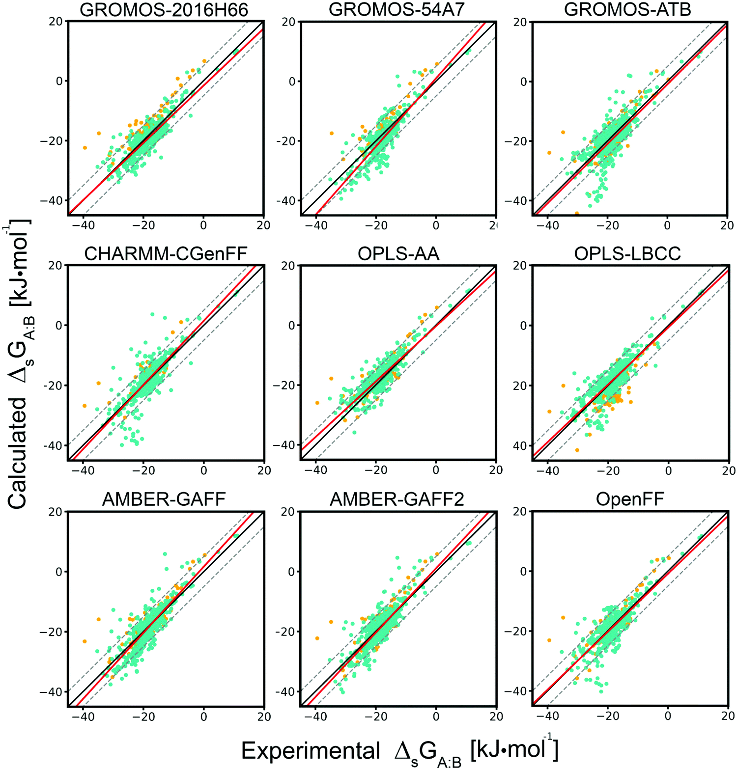Fig. 3 Correlation between experimental and calculated cross-solvation free energies for the nine force fields considered. The individual results (points), the linear-regression line (solid red line), the identity line (solid black line), and the deviation lines (identity ±2k_BT⁻, dashed black lines) are displayed for each of the nine force fields (Table 1). The values are shown for the COMP set (green; N_COMP = 482 points, except GROMOS-54A7 with N_COMP = 399 points) as well as for the extra values of the FULL set (orange; N_FULL − N_COMP points, see Table 1). The numerical values can be found in Section S8 of ref. 43 along with Section S1 (Table S1, ESI†) of the present article. See Table 2 for the associated statistical information.

Table 2 Statistical parameters characterizing the correlation between experimental and calculated cross-solvation free energies for the nine force fields considered, as well as for the single-value and the two-solvent models. The force-field specification includes the force-field family (Fam.) and specific parameter set (Set), see Table 1. The Pearson correlation coefficient (R), the root-mean-square error (RMSE), the average unsigned error (AVUE), and the average error (AVEE) are reported for the FULL set, for the COMP set, and for the CONF set. The total number of simulation points in the COMP set (N_COMP, see Table 1) is also indicated, along with the proportion of calculated solvation free energies in this set that belong to L-Dev (N^L-Dev_COMP; deviation smaller than k_BT⁻), M-Dev (N^M-Dev_COMP; deviation between k_BT⁻ and 2k_BT⁻), and H-Dev (N^H-Dev_COMP; deviation larger than 2k_BT⁻) classes. The corresponding correlations are displayed graphically in Fig. 3. Abbreviation: SMIRNOFF-99Frosst v1.0 (S99F1.0)

Fam.	Set	FULL R	FULL RMSE	FULL AVUE	FULL AVEE	COMP R	COMP RMSE	COMP AVUE	COMP AVEE	N COMP	N ^L-DevCOMP	N ^M-DevCOMP	N ^H-DevCOMP	CONF R	CONF RMSE	CONF AVUE	CONF AVEE
		[kJ mol^−1]				[kJ mol^−1]					[%]	[%]	[%]	[kJ mol^−1]
GROMOS	2016H66	0.84	3.2	2.4	−0.2	0.88	2.9	2.2	−0.8	482	66.4	24.9	8.7	0.92	2.4	1.9	−0.8
GROMOS	54A7	0.85	3.9	2.9	−1.0	0.87	4.0	3.0	−1.5	399	54.6	24.6	20.8	0.90	3.8	2.8	−1.8
GROMOS	ATB	0.75	4.6	3.3	−0.9	0.76	4.8	3.4	−1.0	482	49.4	30.3	20.3	0.83	3.7	2.8	−0.6
CHARMM	CGenFF	0.81	4.1	2.5	+0.4	0.82	4.0	2.4	+0.2	482	70.7	17.6	11.6	0.92	2.6	1.5	+0.5
OPLS	AA	0.87	3.0	2.1	+1.0	0.88	2.9	2.1	+1.0	482	66.4	24.9	8.7	0.92	2.6	1.9	+1.2
OPLS	LBCC	0.81	3.7	2.7	−0.3	0.85	3.3	2.4	+0.2	482	65.3	24.1	10.6	0.91	2.5	2.0	+0.5
AMBER	GAFF	0.85	3.5	2.5	−0.0	0.86	3.6	2.7	−0.2	482	58.3	27.4	14.3	0.91	3.0	2.2	−0.1
AMBER	GAFF2	0.85	3.5	2.5	+0.0	0.86	3.4	2.6	−0.3	482	61.6	26.4	12.0	0.90	2.8	2.1	−0.2
OpenFF	S99F1.0	0.82	3.6	2.5	−0.1	0.82	3.6	2.5	−0.3	482	62.2	25.3	12.5	0.88	2.8	2.1	+0.3
Single-value	—	—	5.3	3.7	0.0	—	5.4	3.9	0.0	482	43.6	33.0	23.4	—	5.4	3.8	0.0
Two-solvent	—	0.73	3.2	2.5	0.0	0.76	3.1	2.5	−0.2	438	57.5	34.0	8.5	0.76	3.0	2.5	−0.3

---

The four force fields already considered in ref. 43 were found to perform comparably well in reproducing the experimental data. The GROMOS-2016H66 and the OPLS-AA force fields have smaller RMSEs (2.9 kJ mol⁻¹) compared to AMBER-GAFF and CHARMM-CGenFF (3.6 and 4.0 kJ mol⁻¹, respectively). However, the AVEEs are slightly smaller in magnitude for AMBER-GAFF and CHARMM-CGenFF (−0.2 and +0.2 kJ mol⁻¹, respectively) compared to GROMOS-2016H66 and OPLS-AA (−0.8 and +1.0 kJ mol⁻¹, respectively). Although GROMOS-2016H66 and OPLS-AA have very similar distributions of errors, AMBER-GAFF has a higher proportion of M-Dev and H-Dev (fewer L-Dev), while CHARMM-CGenFF has a higher proportion of L-Dev and H-Dev (fewer M-Dev). Extending this global comparison to the five additional force fields, the differences remain limited.

Relative to GROMOS-2016H66, both GROMOS-54A7 and GROMOS-ATB present lower correlation coefficients R (0.87 and 0.76, respectively, compared to 0.88) and higher RMSEs (4.0 and 4.8 kJ mol⁻¹, respectively, compared to 2.9 kJ mol⁻¹). The AVEEs of the three sets are negative and of similar magnitudes (−1.5 to −0.8 kJ mol⁻¹), i.e. the GROMOS force fields tend to slightly overestimate the magnitudes of the solvation free energies. Relative to GROMOS-2016H66, GROMOS-54A7 has a significantly higher proportion of H-Dev (fewer L-Dev, similar M-Dev), and GROMOS-ATB a significantly higher proportion of M-Dev and H-Dev (fewer L-Dev).

Relative to OPLS-AA, OPLS-LBCC presents a slightly lower correlation (0.85 compared to 0.88) and a somewhat higher RMSE (3.3 compared to 2.9 kJ mol⁻¹). The distribution of errors is very similar to that of OPLS-AA, with a slightly higher proportion of H-Dev (fewer L-Dev and M-Dev). Whereas the AVEE of OPLS-AA was positive (+1.0 kJ mol⁻¹), suggesting a tendency to slightly underestimate the magnitudes of the solvation free energies, the AVEE for OPLS-LBCC is very close to zero (+0.2 kJ mol⁻¹).

Relative to AMBER-GAFF, AMBER-GAFF2 performs very similarly or slightly better. The correlation coefficient is the same (0.86), the RMSE is marginally lower (3.4 compared to 3.6 kJ mol⁻¹), and the AVEE is also very close to zero (−0.3 compared to −0.2 kJ mol⁻¹). The error distribution is similar as well, with a slightly lower proportion of M-Dev and H-Dev (more L-Dev). Finally, OpenFF presents a lower correlation compared to the AMBER force fields (0.82), together with comparable RMSE and AVEE (3.6 and −0.3 kJ mol⁻¹, respectively), and a similar distribution of errors. This is not entirely surprising, considering the similarity between the Lennard-Jones interaction parameters of OpenFF and AMBER-GAFF for the molecules considered here.

The single-value model (all cross-solvation free energies assumed equal to −18.4 kJ mol⁻¹) presents a RMSE of 5.4 kJ mol⁻¹, larger than the corresponding value for any of the nine force fields (range 2.9–4.8 kJ mol⁻¹). This is reassuring, as it shows that physics-based modeling outperforms this extremely primitive prediction scheme, albeit more or less pronouncedly for the different force fields. The two-solvent model (cross-solvation free energies calculated based on an optimized linear combination of the values for A and B in H₂O and CHE) presents a lower correlation (0.76) compared to the nine force fields considered, but the corresponding RMSE (3.1 kJ mol⁻¹) is actually lower compared to most of the force fields (except GROMOS-2016H66 and OPLS-AA). This observation supports the idea that solvation free energies calculated in two solvent only, one polar and one non-polar, may encompass roughly the same information as a full cross-solvation matrix. The consideration of such a unique solvent pair during force-field refinement, as nowadays commonly done,³² may thus represent a reasonable approximation in the absence of a full cross-solvation matrix. See Section S3 (ESI†) for more details on the calculations involving these two simple models.

Considering the reduced set CONF of highest-confidence experimental data points instead of the COMP set, the correlation with experiment is increased (from the range 0.76–0.88 to the range 0.83–0.92) and the RMSEs are reduced (from the range 2.9–4.8 to the range 2.4–3.8 kJ mol⁻¹). The improvement is most pronounced for CHARMM-CGenFF (4.0 to 2.6 kJ mol⁻¹) and GROMOS-ATB (4.8 to 3.7 kJ mol⁻¹), and least pronounced for GROMOS-54A7 (4.0 to 3.8 kJ mol⁻¹) and OPLS-AA (2.9 to 2.6 kJ mol⁻¹). The trend is systematic for the nine force fields, which suggests that the excluded entries (single value found in the experimental data sources considered) may encompass a higher proportion of less reliable experimental values.

3.2 Comparison for individual compounds

To compare the relative accuracies of the nine force fields for each of the 25 molecules, RMSE and AVEE values were calculated separately for every compound considered either as a solute or as a solvent. The results are shown graphically in Fig. 4 for the COMP set. The corresponding numerical values, as well as analogous material for the FULL set, can be found in Section S2 (Tables S4 and S5, along with Fig. S5, ESI†). In the following discussion, the COMP set is considered in the first place.

Fig. 4 Deviations between experimental and calculated cross-solvation free energies for the nine force fields, considering the set and individual compounds as solute or as solvent. The quantities displayed are (a) the root-mean-square error (RMSE) and (b) the average error (AVEE). Each molecule is considered as solute (blue bars) or as solvent (green bars). The force fields considered are listed in Table 1. The molecules considered and their acronyms are shown in Fig. 1. They are listed in order of decreasing polarity, as estimated by the molecular dipole moment μ. The numerical values can be found in Section S2 (Table S4, ESI†), along with a corresponding comparison considering the FULL set (Table S5 and Fig. S5, ESI†).

The RMSEs of the different compounds considered as solutes or considered as solvents are typically of comparable magnitudes. However, in CHARMM-CGenFF and OpenFF, the RMSEs of the compounds considered as solvents are larger for most molecules. In CHARMM-CGenFF, the AVEEs of both types are also noticeably smaller in magnitude compared to the eight other force fields, except for a number of outliers (most prominently DAMD, DEAN, and TEAN as solutes). The RMSEs of both types are tendentially larger in GROMOS-ATB and, to a lesser extent, GROMOS-54A7 compared to GROMOS-2016H66. The two sets also present a more pronounced (though non-systematic) sign bias towards negative AVEEs, i.e. indicative of solvation free energies that tend to be overestimated in magnitude. In the opposite, OPLS-AA presents a (non-systematic) sign bias towards positive AVEEs, i.e. indicative of solvation free energies that tend to be underestimated in magnitude. This trend is no longer visible for OPLS-LBCC. Note, however, that the absence of sign bias in the global AVEE for OPLS-LBCC, AMBER-GAFF, AMBER-GAFF2, and OpenFF, is in part fortuitous, as it results from the partial cancellation of larger positive and negative AVEEs over the present selection of compounds.

Dimethylacetamide (DAMD) as solute consistently presents large RMSEs (4.7 to 13.6 kJ mol⁻¹) along with negative AVEEs (−13.2 to −4.2 kJ mol⁻¹). The solvation free energy of this molecule is thus tendentially overestimated in magnitude for all solvents and force fields. The same applies to a lesser extent to ethyl acetate (EAE), which also presents relatively large RMSEs (2.0 to 8.7 kJ mol⁻¹) and tendentially negative AVEEs (−8.3 to +0.3 kJ mol⁻¹). Note, however, that the RMSEs for these two compounds as solvents are not anomalously high, and present no significant sign bias. For DAMD as a solute, these discrepancies might result in part from less accurate experimental data (for this compound as solute one has either a single experimental value or multiple values with a large spread, see Fig. 2b).

Water (H₂O) is associated with comparable and relatively large RMSEs as solute (3.8 to 5.5 kJ mol⁻¹) and as solvent (2.7 to 6.4 kJ mol⁻¹). The corresponding AVEEs are nearly systematically positive (+0.4 to +3.0 kJ mol⁻¹ as solute, −0.3 to +3.7 kJ mol⁻¹ as solvent), i.e. the solvation free energies involving H₂O as solute or as solvent are tendentially underestimated in magnitude by all force fields. For H₂O as solvent, the best agreement with experiment is obtained for the GROMOS-2016H66 force field, with values of 2.7 and +0.8 kJ mol⁻¹ for the RMSE and AVEE, respectively. This is in line with the fact that hydration free energies have been included as target during the force-field calibration.³² In contrast, GROMOS-54A7, GROMOS-ATB, and CHARMM-CGenFF present the largest discrepancies, with RMSEs of 5.6, 6.0, and 6.4 kJ mol⁻¹, respectively. The corresponding AVEEs are positive (+1.2 to +2.2 kJ mol⁻¹), i.e. the magnitudes of the hydration free energies tend to be underestimated by these three force fields. For AMBER-GAFF2 and OpenFF, the RMSEs are similar to those for AMBER-GAFF (5.4 and 5.2 kJ mol⁻¹, respectively, compared to 5.5 kJ mol⁻¹). The corresponding AVEEs are also positive (+2.1 to +2.9 kJ mol⁻¹), i.e. the magnitudes of the hydration free energies tend also here to be underestimated. Finally, for OPLS-LBCC, the RMSE is smaller than for OPLS-AA (3.2 compared to 4.6 kJ mol⁻¹), and the AVEE is now very close to zero (−0.3 compared to +3.7 kJ mol⁻¹). Thus, although the magnitudes of the hydration free energies tend to be underestimated by OPLS-AA, this bias is removed in OPLS-LBCC. This is in line with the fact that the 1.14 × CM1A-LBCC charge-derivation scheme involves an empirical upscaling of the charges by a factor of 1.14 and the use of localized bond-charge corrections which are optimized precisely to improve agreement with the experimental hydration free energies.^68,95,96

The amines (ANLN, DEAN, and TEAN), which can be challenging compounds in terms of force-field design,^{61,120,156,157} also tend to have relatively large errors compared to experiment, both as solutes and as solvents. However, the extent of disagreement varies from force field to force field, with AVEEs of different signs. For these three compounds, the RMSEs of both types are generally somewhat larger in GROMOS-54A7 and GROMOS-ATB (3.3 to 6.6 kJ mol⁻¹; see, however, ref. 157 for a recent GROMOS-compatible reparametrization) compared to GROMOS-2016H66 (2.7 to 5.6 kJ mol⁻¹). They are also large in CHARMM-CGenFF (2.7 to 8.4 kJ mol⁻¹), especially for DEAN. The smallest RMSEs for the three compounds are obtained for OPLS-LBCC (2.2 to 4.4 kJ mol⁻¹) and OpenFF (2.3 to 4.6 kJ mol⁻¹). Here, OPLS-LBCC performs slightly better than OPLS-AA (2.3 to 5.5 kJ mol⁻¹), and OpenFF slightly better than AMBER-GAFF and AMBER-GAFF2 (3.7 to 5.9 kJ mol⁻¹). For DEAN as solvent and, to a lesser extent, TEAN as solvent, these discrepancies might result in part from less accurate experimental data (for the different solutes in these two solvents, one has mostly or exclusively a single experimental value, see Fig. 2b).

For the alcohols (PTL, MTL, ETL, BTL, 2M2P, 1PL, and 2PL), both as solutes and as solvents, four sets are affected by comparatively large errors. The RMSEs are larger in GROMOS-ATB (2.3 to 7.0 kJ mol⁻¹) and, to a lesser extent, in GROMOS-54A7, CHARMM-CGenFF and OpenFF (1.6 to 5.2 kJ mol⁻¹) compared to the five other parameter sets (1.4 to 4.4 kJ mol⁻¹). The signs and magnitudes of the corresponding AVEEs differ significantly and non-systematically depending on the compound, its consideration as solute or as solvent, and the chosen force field.

For the chlorinated compounds (CHCL3, CCL4, and C2CL2), which were omitted from the COMP set, the FULL set must be considered (Fig. S5, ESI†), keeping in mind that some of these molecules are unavailable in specific force fields (Table 1). For this class of compounds, considered both as solutes and as solvents, OPLS-LBCC stands out as presenting comparatively large RMSEs (3.5 to 6.3 kJ mol⁻¹) along with tendentially negative AVEEs (−5.5 to −0.8 kJ mol⁻¹). The eight other force fields present smaller RMSEs (1.8 to 4.1 kJ mol⁻¹) and less sign bias in the AVEEs (−2.6 to +2.9 kJ mol⁻¹).

The GROMOS-2016H66 parameters set³² is the only one that has included solvation free energies in an apolar solvent, cyclohexane (CHE), as a calibration target. Interestingly, however, the eight other force fields reproduce similarly well the solvation free energies in CHE, with RMSEs ranging between 1.9 and 3.2 kJ mol⁻¹, compared to 2.3 kJ mol⁻¹ for GROMOS-2016H66. In the nine force fields, the solvation free energies in the two other aliphatic non-polar solvents hexane and heptane (HXE and HPE) show similar deviations compared to CHE, with RMSEs between 1.8 and 3.5 kJ mol⁻¹. The solvation free energies in the non-polar aromatic solvents benzene and toluene (BZN and TOL) also present relatively small RMSEs in the nine force fields, ranging between 2.0 and 4.3 kJ mol⁻¹. Note that although the errors affecting the solvation free energies in the five non-polar solvents (green bars for TOL-CHE in Fig. 4) show little variations across solvents and force fields, the variability is significantly more pronounced when these non-polar molecules are considered as solutes (corresponding blue bars).

3.3 Comparison for individual compound pairs

The differences between experimental and calculated cross-solvation free energies for all pairs of compounds are shown in Fig. 5 for the nine force fields. Corresponding matrices for the calculated solvation free energies as well as their electrostatic component ΔG_ELE and van der Waals component ΔG_VDW are also shown in Section S8 of ref. 43 (Fig. S10–S12 therein) for the four force fields already considered in the previous article, and in Section S1 (Fig. S1–S3, ESI†) for the five force fields newly considered. Note that unlike the total free energy changes, the components ΔG_ELE and ΔG_VDW are path-dependent quantities,^158,159 which are of theoretical relevance, but do not correspond to experimental observables. Of particular interest here is the observation that ΔG_VDW is negative for almost all pairs, except those involving water (H₂O) either as solute or as solvent, and a few instances involving methanol (MTL) as solute. The component ΔG_ELE is nearly always negative as well, except for 38 instances of positive values in GROMOS-ATB (typically less than +1.0 kJ mol⁻¹ and up to +3.9 kJ mol⁻¹ at most), all of which involve LP solutes or LP solvents. This component is tendentially larger in magnitude for pairs involving only HP or MP compounds, and particularly negative for the pairs involving H₂O either as solute or as solvent. Note also the strong similarity in the ΔG_VDW matrices of AMBER-GAFF and OpenFF, which follows from the similarity between the Lennard-Jones interaction parameters of these two force fields for the molecules considered here, and implies that the main differences in solvation free energies arise from the ΔG_ELE component via the different partial charges.

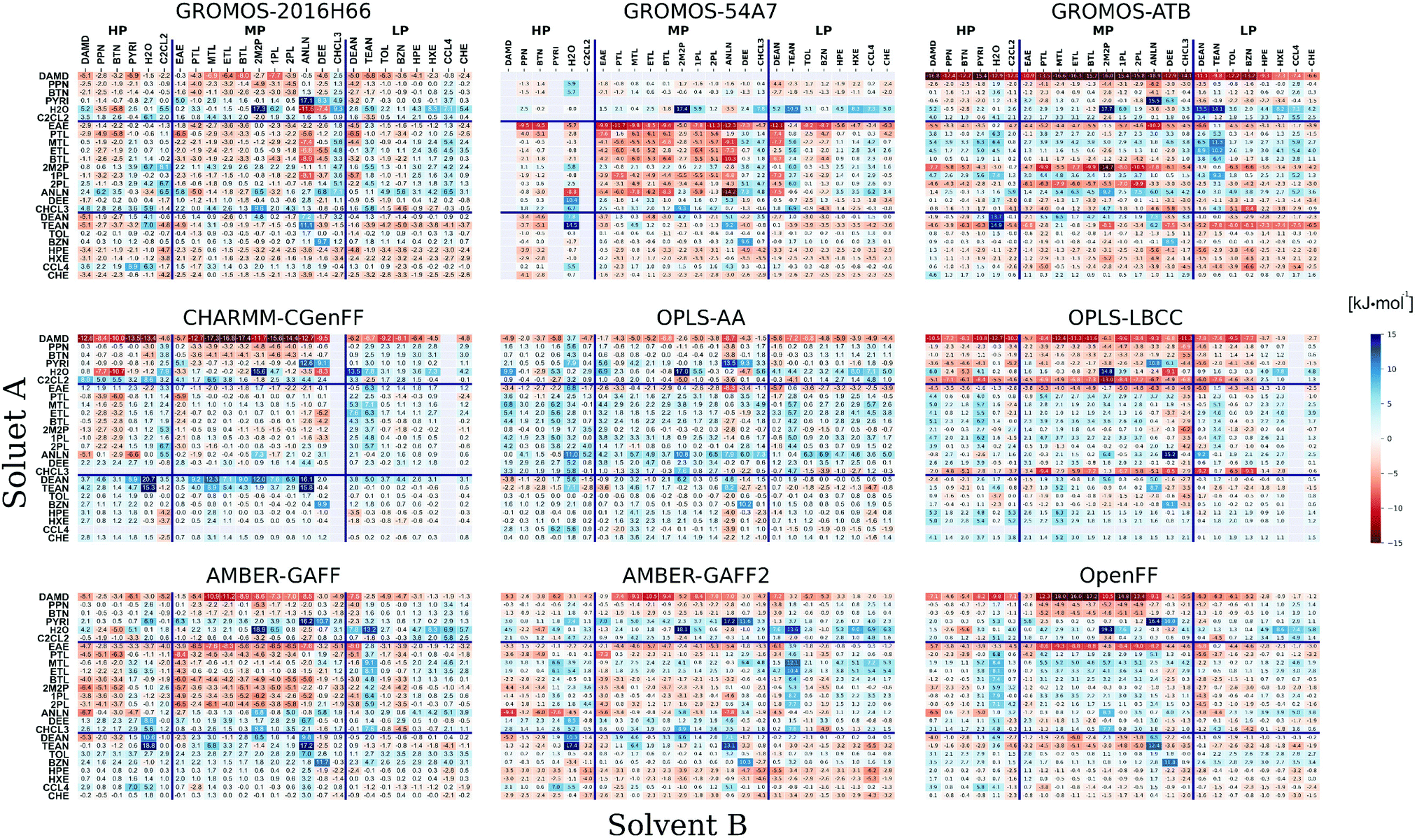Fig. 5 Deviations between experimental and calculated cross-solvation free energies for the nine force fields considered. The deviations (calculation minus experiment) are given for the solutes A (rows) in the solvents B (columns). The force fields considered are listed in Table 1. The molecules considered and their acronyms are shown in Fig. 1. They are listed along the rows and columns in order of decreasing polarity, as estimated by the molecular dipole moment μ, and the partitioning into low (LP), medium (MP), and high (HP) polarity categories is also indicated (see Fig. 1). The corresponding numerical values can be found in Section S8 of ref. 43 along with Section S1 (Table S3, ESI†) of the present article. The calculated solvation free energies, their electrostatic components and their van der Waals components are displayed in Fig. S1–S3 (ESI†), respectively.

Considering Fig. 5, the compound DAMD as a solute clearly represents a challenging case for most force fields (except GROMOS-54A7, which includes no parametrization for this compound). In GROMOS-ATB and, to a lesser extent, CHARMM-CGenFF, the magnitude of the solvation free energy of this compound in all solvents is dramatically overestimated, with errors that range between −6.6 and −18.9 kJ mol⁻¹, and are particularly large in the MP solvents. For OPLS-LBCC, AMBER-GAFF, AMBER-GAFF2, and OpenFF, important deviations are observed as well in the MP solvents, with errors that can reach −18.0 kJ mol⁻¹. In GROMOS-ATB, the negative error is mainly due to an overly negative ΔG_VDW. In the five other cases, it is related to an overly negative ΔG_ELE, resulting from high negative partial charges on the nitrogen and oxygen atoms, more pronouncedly so for CHARMM-CGenFF, OPLS-LBCC, and OpenFF. Interestingly, all the above force fields rely on atomic partial charges derived based on QM calculations. In contrast, GROMOS-2016H66 and OPLS-AA, in which the charges are empirically fitted to reproduce experimental data, lead to smaller (yet still sizeable) errors of at most −8.0 and −8.7 kJ mol⁻¹, respectively. Note that the above discrepancies might also result in part from less accurate experimental data for DAMD as a solute (see Fig. 2b). The solute EAE also tends to present large and negative errors in GROMOS-54A7, GROMOS-ATB, AMBER-GAFF, and OpenFF with deviations that can reach −12.3, −10.2, −8.3, and −9.3 kJ mol⁻¹, respectively. However, this solute does not appear to be particularly problematic in the five other force fields.

Considering water as a solvent, GROMOS-2016H66 and OPLS-LBCC present the best agreement with experiment, with deviations of at most 7.0 and 5.5 kJ mol⁻¹ in magnitude, respectively (excluding the solute DAMD for OPLS-LBCC), in line with the consideration of hydration free energies as targets during the parametrization of these two force fields.^32,68,95,96 The seven other force fields also reproduce the hydration free energies reasonably well, with a number of exceptions: (i) OPLS-AA nearly systematically presents positive deviations, a feature that disappears when using the higher charges of OPLS-LBCC; (ii) GROMOS-54A7, GROMOS-ATB, CHARMM-CGenFF, OPLS-AA, AMBER-GAFF, and AMBER-GAFF2 present markedly too positive values for the aliphatic amines (DEAN and TEAN), mainly due to low atomic partial charges in these molecules; (iii) GROMOS-2016H66, GROMOS-54A7, OPLS-AA, AMBER-GAFF, AMBER-GAFF2, and OpenFF present large positive deviations for CHCL3 (all) and DEE (all except GROMOS-2016H66); (iv) GROMOS-54A7 and OPLS-AA present large deviations (of opposite signs) for ANLN; (v) The values for the alcohols are slightly less negative in AMBER-GAFF2 (deviations from −0.5 to +5.4 kJ mol⁻¹) and markedly more positive in OpenFF (from +5.9 to +8.4 kJ mol⁻¹), compared to AMBER-GAFF (−1.2 to +3.5 kJ mol⁻¹).

The solvation free energies of alcohols in alcohols are most accurately reproduced by CHARMM-CGenFF (deviation from −1.6 to +1.5 kJ mol⁻¹) and, to a lesser extent, GROMOS-2016H66 (−4.3 to +4.3 kJ mol⁻¹) and AMBER-GAFF2 (−3.7 to +4.1 kJ mol⁻¹). The same applies for GROMOS-ATB as well (from −4.2 and +4.8 kJ mol⁻¹) if one excepts the secondary (2PL) and tertiary (2M2P) alcohols as solutes (deviations of −9.9 and −14.7 kJ mol⁻¹, respectively). In contrast, the values are tendentially affected by negative errors in GROMOS-54A7 and AMBER-GAFF (down to −7.5 kJ mol⁻¹), and by positive errors in OPLS-AA, OPLS-LBCC, and OpenFF (up to +5.7 kJ mol⁻¹). The difference between these two groups of force fields for the alcohols can be explained by considering the Lennard-Jones interaction parameters. Both the oxygen atom and the alpha carbon atom have smaller σ and larger ε values in AMBER-GAFF compared to OPLS-AA and OPLS-LBCC. Similarly, the oxygen atom has a smaller repulsive C₁₂ and a larger attractive C₆ in GROMOS-54A7 compared to GROMOS-2016H66, along with a slightly more negative charge. These changes enhance the attractive solute–solvent interactions directly, but also indirectly via an enhancement of the hydrogen-bonding interactions due to shorter donor–acceptor distances. A similar change of Lennard-Jones interaction parameters (oxygen atom more repulsive with a larger σ and a smaller ε, aliphatic hydrogen atom more attractive with a smaller σ and a slightly larger ε) also explains why AMBER-GAFF2 performs better here than AMBER-GAFF. In OpenFF, the partial charges on the oxygen atom, the hydroxyl hydrogen and the alpha carbon atom are too small compared to AMBER-GAFF. The resulting less attractive electrostatic interactions between the alcohols explains the positive deviations in the OpenFF force field.

The amines (DEAN, TEAN, and ANLN) are associated with large deviations from experiment in specific parameter sets. This is in particular the case for the solvation free energies in ANLN considering the solutes PYRI and TEAN (and, to a lesser extent, DEAN), which are associated with large positive errors in all force fields (up to 17.2 kJ mol⁻¹), and considering the MP solutes in GROMOS-2016H66, GROMOS-54A7, and AMBER-GAFF, which are associated with predominantly negative errors (down to −14.2 kJ mol⁻¹). The solvation free energies in DEAN and TEAN are also characterized by particularly large deviations in GROMOS-54A7, GROMOS-ATB, CHARMM-CGenFF, AMBER-GAFF, and AMBER-GAFF2 (up to 14.1 kJ mol⁻¹ in magnitude, tendentially more positive for TEAN compared to DEAN). These issues do not affect the four other force fields as significantly (errors up to 9.2 kJ mol⁻¹ in magnitude). Note that the above discrepancies might also result in part from less accurate experimental data for DEAN as solvent and, to a lesser extent, TEAN as solvent (see Fig. 2b). Finally, the solvation free energies involving DEAN and TEAN as solutes are associated with large positive errors in CHARMM-CGenFF (up to 16.1 kJ mol⁻¹, excepting the solvent H₂O), and negative errors in GROMOS-ATB (down to −8.1 kJ mol⁻¹), especially for TEAN and in the LP solvents. These issues do not affect the seven other force fields as significantly (errors up to 6.8 kJ mol⁻¹ in magnitude, excepting the solvents H₂O and ANLN).

Except in combination with some of the exceptional solutes and solvents mentioned above, the solvation free energies involving apolar molecules (TOL, BZN, HPE, HXE, CCL4 and CHE), both as solute and as solvent, present less pronounced discrepancies in all nine force fields. The corresponding errors do not exceed 7.2 kJ mol⁻¹ in magnitude, excluding the solutes DAMD, H₂O, EAE, CHCL3, and TEAN, as well as the solvents DEE and PYRI.

It is interesting to note that the force-field adjustments made from OPLS-AA to OPLS-LBCC (different charge set) or from AMBER-GAFF to AMBER-GAFF2 (adjusted covalent terms and Lennard-Jones parameters) induce conflicting effects on different solute–solvent pairs. For example, the change from OPLS-AA to OPLS-LBCC noticeably improves the accuracy of the hydration free energies (increase in magnitude due to higher solute charges), but also results in a tendency to overestimate the solvation free energies of polar solutes in other polar solvents. This affects in particular the solutes DAMD, PYRI, C2CL2, EAE, and CHCL3 in the non-aqueous polar solvents and MP solvents and, to a lesser extent, the solutes PPN and BTN in the MP solvents. Similarly, the accuracy of the solvation free energies of alcohols in alcohols (and in a few other solvents as well) is improved by the change from AMBER-GAFF to AMBER-GAFF2 (more repulsive oxygen atom, more attractive aliphatic hydrogen atom), but the change also induces positive shifts in the solvation free energies of MTL and ETL in CHE, CCL4, HXE, and PYRI (deviations from +5.1 to +7.2 kJ mol⁻¹vs. +2.1 to +4.6 kJ mol⁻¹ for AMBER-GAFF), and negative shifts in the solvation free energies of the aliphatic apolar solutes HPE, HXE, and CHE in all solvents (from −6.2 to 0.0 kJ mol⁻¹vs. −2.8 to +3.2 kJ mol⁻¹ for AMBER-GAFF).

3.4 Transfer free energies

The level of agreement between experiment and simulation in terms of the cross-solvation free energies does not automatically imply a corresponding level of agreement in terms of transfer (partitioning) free energies between two solvents, defined as , because deviations can add up or, in the opposite, partly compensate each other. The RMSEs over all solutes C of the transfer free energies of a given solute C from solvent A to solvent B are shown in matrix form for the COMP set in Fig. 6. The corresponding results for the FULL set are displayed in Section S1 (Fig. S4, ESI†). These matrices are symmetric, and only the upper triangle is shown. The averages of these RMSEs over all pairs are noticeably lower for OPLS-AA, OPLS-LBCC, and GROMOS-2016H66 (2.7, 2.9 and 3.1 kJ mol⁻¹) compared to the six other force fields (3.5 to 3.9 kJ mol⁻¹).

Fig. 6 Root-mean-square error relative to experiment for the transfer free energies of all solutes C between any pair of solvents A and B considering the COMP set. For each solvent pair, the RMSE of is obtained by considering the entire series of solutes C. The force fields considered are listed in Table 1. The molecules considered and their acronyms are shown in Fig. 1. They are listed along the rows and columns in order of decreasing polarity, as estimated by the molecular dipole moment μ, and the partitioning into low (LP), medium (MP), and high (HP) polarity categories is also indicated (see Fig. 1). The corresponding numerical values can be found in Section S8 of ref. 43 along with Section S1 (ESI†) of the present article. The analog of this figure for the FULL set is provided in Section S1 (Fig. S4, ESI†).

The solvent pairs involving ANLN and DEE present high RMSEs for all nine force fields (up to 8.9 kJ mol⁻¹), possibly hinting at larger errors affecting the corresponding experimental values. Besides these two solvents, GROMOS-54A7, GROMOS-ATB, CHARMM-CGenFF, AMBER-GAFF, AMBER-GAFF2, and OpenFF are affected by large RMSEs for the pairs involving TEAN (up to 7.7 kJ mol⁻¹, excluding pairs with ANLN and DEE). For GROMOS-ATB and CHARMM-CGenFF, the same applies to the pairs involving DEAN (up to 7.0 kJ mol⁻¹). In GROMOS-2016H66 and OPLS-LBCC (and, to lesser extent, OPLS-AA), the RMSEs for the pairs involving H₂O present smaller errors (generally below 5.0 kJ mol⁻¹) compared to the six other force fields (generally above 5.0 kJ mol⁻¹).

Two examples of error compensation within are the following. First, AMBER-GAFF has slightly larger errors compared to AMBER-GAFF2 in terms for the solvation of the various solutes in the alcohols (Fig. 5). However, in AMBER-GAFF, the errors evidence more similar deviation patterns along the solute series when comparing the different alcohol solvents. As a result, AMBER-GAFF and AMBER-GAFF2 still perform similarly well in reproducing the transfer free energies between alcohols. Second, although GROMOS-ATB presents larger errors than all the other force fields in terms of (Table 2 and Fig. 5), it still reproduces the with an accuracy comparable to that of five other force fields (the average RMSE of the matrix for this force field is 3.6 kJ mol⁻¹). These observations emphasize the importance of considering both solvation free energies and transfer free energies when evaluating the relative accuracies of force fields.

3.5 Extent of consensuality between force fields

The consensus root-mean-square error matrix, defined by the root-mean-square deviation from experiment considering the sets of values obtained using the nine force fields simultaneously, is shown in Fig. 7a. The observation of a low RMSE for most of the entries indicates that the majority of the force fields can accurately reproduce the corresponding solvation free energy.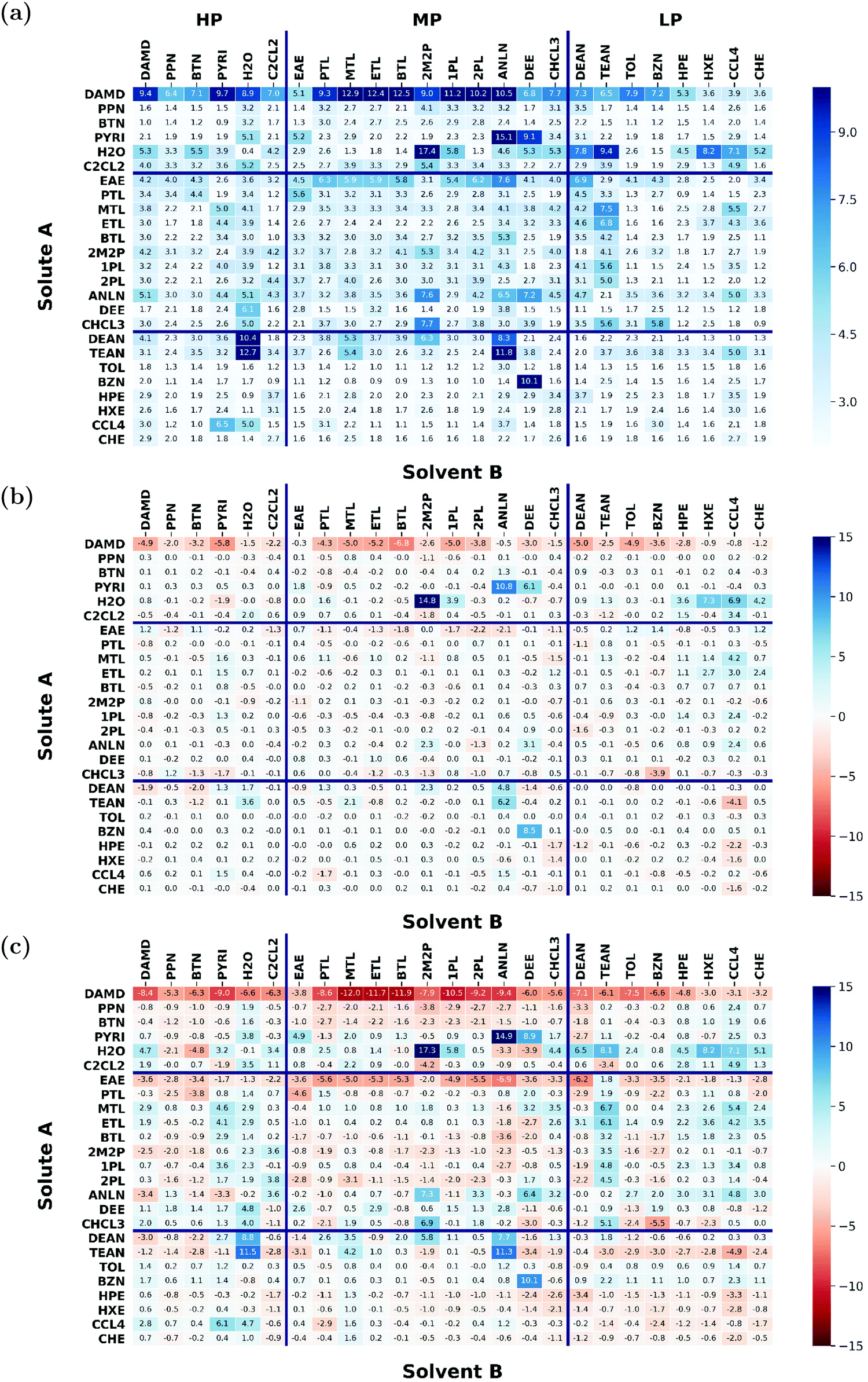

Fig. 7 The consensus root-mean-square error matrix, defined as the root-mean-square deviation from experiment considering the nine force fields simultanously (a), the consensus minimum-error matrix, defined as the smallest deviation (in magnitude) from experiment achieved by any one of the nine force fields considered (b), and the consensus average-error matrix, defined as the deviation from experiment of the average over the nine force fields (c). The force fields considered are listed in Table 1. The molecules considered and their acronyms are shown in Fig. 1. They are listed along the rows and columns in order of decreasing polarity, as estimated by the molecular dipole moment μ. The deviations between experimental and calculated cross-solvation free energies for each of the nine force fields are displayed in Fig. 5. The corresponding numerical values can be found in Section S8 of ref. 43 along with Section S1 (Table S3, ESI†) of the present article.

The consensus minimum-error matrix, defined by the smallest deviation (in magnitude) from experiment achieved by any one of the nine force fields considered, is shown in Fig. 7b. This matrix has an RMSE of 1.4 kJ mol⁻¹ over all its entries (expectedly smaller than the value of 1.6 kJ mol⁻¹ obtained previously⁴³ when considering only four force fields). Thus, by choosing the best possible force field on a case to case basis, one can very accurately reproduce the vast majority of the experimental solvation free energies. However, there are several instances where the calculated cross-solvation free energy of a given solute–solvent pair substantially deviates from experiment regardless of the force field employed. The fact that each of the nine force fields fails to reproduce the experimental value might be an indication of an error in the experimental data, although it may also result from an inaccuracy of the molecular model underlying all these force fields (e.g. classical-mechanics approximation or absence of explicit electronic polarization). The solvation free energies of H₂O in 2M2P and of PYRI in ANLN are two examples with possibly large experimental errors, both of which were excluded from the COMP set (see Appendix A of ref. 43 for a possible alternative experimental value in the case of H₂O:2M2P). There are 11 other cases with errors of 2k_BT⁻ or larger in this matrix (expectedly fewer than the 18 cases observed previously⁴³ when considering only four force fields), namely DAMD:PYRI, DAMD:MTL, DAMD:ETL, DAMD:BTL, DAMD:1PL, DAMD:DEAN, PYRI:DEE, H₂O:HXE, H₂O:CCL4, TEAN:ANLN, and BZN:DEE. In the majority of these cases, the experimental data has either a single value reported in the literature, or significant experimental discrepancies among the different values reported. The validity of this experimental data can therefore indeed be questioned.

Finally, the consensus average-error matrix, defined by the deviation from experiment of the average solvation free energy over the nine force fields, is displayed in Fig. 7c. The matrix shows the extent of error cancellation upon averaging the results over the force fields. This matrix has an RMSE of 3.0 kJ mol⁻¹ over all its entries, expectedly larger than the corresponding value of 1.4 kJ mol⁻¹ for the minimum-error matrix. However, it is also larger than the lowest single force-field RMSEs of 2.9 kJ mol⁻¹ obtained for GROMOS-2016H66 and OPLS-AA (Table 2). Thus, it remains better to choose a force field expected to present the highest possible accuracy for the compound class of interest than to average the results over a set of arbitrary force fields.

4 Conclusions

Experimental solvation free energies are nowadays commonly included as target properties in the validation of condensed-phase force fields, sometimes even in their calibration. The involved comparison between experimental values and simulation results can be made more systematic by considering a full matrix of cross-solvation free energies⁴³. For a selected set of N molecules, this N × N matrix probes on an equal footing the interactions of each molecule in the set with a surrounding consisting of the bulk liquid of each molecule (other or self) in the set. Provided that the compound set is sufficiently diverse in terms of chemical functional groups (i.e. encompasses a number of compounds representative of each relevant chemical function), this data accounts in a comprehensive and balanced fashion for the intermolecular interactions that should be accurately represented by the force field.

In our previous article,⁴³ a cross-solvation matrix of 25 × 25 experimental value was introduced by collecting and curating data from seven literature sources,^47–53 including compounds from one to seven carbon atoms representative for alkanes, chloroalkanes, ethers, ketones, esters, alcohols, amines, and amides. This experimental data was used to compare the relative accuracies of four popular condensed-phase force fields, namely GROMOS-2016H66, OPLS-AA, AMBER-GAFF, and CHARMM-CGenFF. In the present work, this comparison is extended to five additional force fields, namely GROMOS-54A7, GROMOS-ATB, OPLS-LBCC, AMBER-GAFF2, and OpenFF.

Considering these nine force fields, the correlation coefficients between experimental values and simulated results range from 0.76 to 0.88, the RMSEs from 2.9 to 4.8 kJ mol⁻¹, and the AVEEs from −1.5 to +1.0 kJ mol⁻¹. These differences are statistically significant, but not very pronounced, especially considering the very different functional-form choices and parametrization strategies of the nine force fields as well as the influence of outliers, some of which possibly caused by inaccurate experimental data. Considering the RMSEs, GROMOS-2016H66 and OPLS-AA present the best accuracy (2.9 kJ mol⁻¹), followed by OPLS-LBCC, AMBER-GAFF2, AMBER-GAFF, and OpenFF (3.3 to 3.6 kJ mol⁻¹), and then by GROMOS-54A7, CHARM-CGenFF, and GROMOS-ATB (4.0 to 4.8 kJ mol⁻¹). Considering the AVEEs, the three GROMOS force fields tend to slightly overestimate the magnitudes of the solvation free energies (−1.5 to −0.8 kJ mol⁻¹). In the opposite, the OPLS-AA force field shows a slight tendency to underestimate the magnitudes of the solvation free energies (+1.0 kJ mol⁻¹). The five other force fields show no significant sign bias (AVEEs between −0.3 and +0.2).

As shown by further analysis of the RMSEs and AVEEs in terms of solutes, solvents, and solute–solvent pairs, these global errors are distributed somewhat heterogeneously over the different compounds within the different force fields. In particular, the above trends in terms of global AVEEs may result at least in part from the fortuitous cancellation of larger positive and negative errors over the present selection of compounds. It is also observed that GROMOS-2016H66 and OPLS-LBCC present smaller errors in the hydration free energies, in line with the fact that these parameter sets included hydration free energies as targets in their calibration.

The errors affecting the solvation free energies in the five non-polar solvents show remarkably little variations across solvents and force fields. However, this observation does not imply that the nine force fields are essentially equivalent with respect to their description of the Lennard-Jones interactions, and that variations of the solvation free energy in more polar solvents only arise from differences in the atomic charges. First, the variability is significantly more pronounced when the non-polar molecules are considered as solutes. Second, for polar molecules, the repulsive Lennard-Jones interaction parameters are largely correlated with the charges, because it is their balance that determines the geometry and strength of favorable polar interactions (e.g. hydrogen bonds). Furthermore, the Lennard-Jones parameters of the non-polar and polar molecules are connected by the application of combination rules, as well as correlated with other simulation choices (e.g. cutoff distances, treatment of the long-range non-bonded interactions). A consequence of these observations is that the simultaneous optimization of Lennard-Jones parameters and atomic charges in force-field refinement is to be preferred over a sequential one.^32,124,160

The present study also underlines three points related to the extensive comparison between experiment and simulation results in terms of solvation free energies. First, the importance of considering both solvation free energies and transfer free energies when evaluating the relative accuracies of force fields, so as to avoid biases related to error enhancement or compensation. Second, the fact that choosing a force field expected to present the highest possible accuracy for the compound class of interest remains a better strategy compared to averaging the results obtained using an arbitrary set of force fields. And finally, that such systematic comparisons between simulation and experiment and, in particular, the minimum-error matrix over all force fields considered, may be extremely useful for detecting suspicious (i.e. possibly erroneous) experimental values.

Cross-solvation matrices are expected to represent a powerful tool not only for force-field validation/comparison, but also for force-field refinement/calibration. This is because such a matrix includes a large number of observables which probe all the pair-type interactions relevant for the force field in a balanced fashion. Owing to these two features, this target data may be particularly well suited for assessing the relative merits of different van der Waals combination rules and charge-derivation schemes, and the possibility of bypassing them when necessary using pair-specific parameters or empirical scaling factors.

In the near future, this work related to cross-solvation matrices will be expanded along three main directions: (i) further expansion and curation of the experimental data set; (ii) use of cross-solvation matrices in force-field calibration (e.g. in the context of the systematic CombiFF force-field refinement approach^124,160); (iii) extension to liquid–liquid mixing properties at finite concentration.

Conflicts of interest

There are no conflicts to declare.

Acknowledgements

Financial support by the Swiss National Science Foundation (Grant No. 200021-175944) is gratefully acknowledged.

References

1. D. L. Mobley, E. Dumont, J. D. Chodera and K. A. Dill, J. Phys. Chem. B, 2007, 111, 2242–2254.
2. D. L. Mobley, C. I. Bayly, M. D. Cooper, M. R. Shirts and K. A. Dill, J. Chem. Theory Comput., 2009, 5, 350–358.
3. S. Shivakumar, Y. Deng and B. Roux, J. Chem. Theory Comput., 2009, 5, 919–930.
4. D. Shivakumar, J. Williams, Y. Wu, W. Damm, J. Shelley and W. Sherman, J. Chem. Theory Comput., 2010, 6, 1509–1519.
5. D. Shivakumar, E. Harder, W. Damm, R. A. Friesner and W. Sherman, J. Chem. Theory Comput., 2012, 8, 2553–2558.
6. P. S. Nerenberg, B. Jo, C. So, A. Tripathy and T. Head-Gordon, J. Phys. Chem. B, 2012, 116, 4524–4534.
7. L. Huang and B. Roux, J. Chem. Theory Comput., 2013, 9, 3543–3556.
8. J. P. M. Jämbeck and A. P. Lyubartsev, J. Phys. Chem. B, 2014, 118, 3793–3804.
9. M. Lundborg and E. Lindahl, J. Phys. Chem. B, 2015, 119, 810–823.
10. J. Zhang, B. Tuguldur and D. van der Spoel, J. Chem. Inf. Model., 2015, 55, 1192–1201.
11. J. Zhang, B. Tuguldur and D. van der Spoel, J. Chem. Inf. Model., 2016, 56, 819–820.
12. H. Zhang, C. Yin, Y. Jiang and D. van der Spoel, J. Chem. Inf. Model., 2018, 58, 1037–1052.
13. C. L. Wennberg, T. Murtola, S. Páll, M. J. Abraham, B. Hess and E. Lindahl, J. Chem. Theory Comput., 2015, 11, 5737–5746.
14. N. M. Fischer, P. J. van Maaren, J. C. Ditz, A. Yildirim and D. van der Spoel, J. Chem. Theory Comput., 2015, 11, 2938–2944.
15. Z. Bashardanesh and D. van der Spoel, J. Phys. Chem. B, 2018, 122, 8018–8027.
16. Y. M. H. Gonçalves, C. Senac, P. F. J. Fuchs, P. H. Hünenberger and B. A. C. Horta, J. Chem. Theory Comput., 2019, 15, 1806–1826.
17. S. W. Siu and K. Pluhackova, J. Chem. Theory Comput., 2012, 8, 1459–1470.
18. M. Fyta and R. R. Netz, J. Chem. Phys., 2012, 136, 124103.
19. J. Yoo and A. Aksimentiev, J. Phys. Chem. Lett., 2012, 3, 45–50.
20. J. Yoo and A. Aksimentiev, J. Chem. Theory Comput., 2016, 12, 430–443.
21. V. Satarifard, S. Kashefolgheta, A. Vila Verde and A. Grafmüller, J. Chem. Theory Comput., 2017, 13, 2112–2122.
22. S. Kashefolgheta and A. Vila Verde, Phys. Chem. Chem. Phys., 2017, 19, 20593–20607.
23. J. Huang, S. Rauscher, G. Nawrocki, T. Ran, M. Feig, B. L. de Groot, H. Grubmüller and A. D. MacKerell Jr, Nat. Methods, 2017, 14, 71–73.
24. E. Boulanger, L. Huang, C. Rupakheti, A. D. MacKerell Jr. and B. Roux, J. Chem. Theory Comput., 2018, 14, 3121–3131.
25. A. Krämer, F. C. Pickard IV, J. Huang, R. M. Venable, A. C. Simmonett, D. Reith, K. N. Kirschner, R. W. Pastor and B. R. Brooks, J. Chem. Theory Comput., 2019, 15, 3854–3867.
26. C. Oostenbrink, A. Villa, A. E. Mark and W. F. van Gunsteren, J. Comput. Chem., 2004, 25, 1656–1676.
27. N. Schmid, A. P. Eichenberger, A. Choutko, S. Riniker, M. Winger, A. E. Mark and W. F. van Gunsteren, Eur. Biophys. J., 2011, 40, 843–856.
28. B. A. C. Horta, P. F. J. Fuchs, W. F. van Gunsteren and P. H. Hünenberger, J. Chem. Theory Comput., 2011, 7, 1016–1031.
29. B. A. C. Horta, Z. Lin, W. Huang, S. Riniker, W. F. van Gunsteren and P. H. Hünenberger, J. Comput. Chem., 2012, 33, 1907–1917.
30. P. F. J. Fuchs, H. S. Hansen, P. H. Hünenberger and B. A. C. Horta, J. Chem. Theory Comput., 2012, 8, 3943–3963.
31. M. M. Reif, P. H. Hünenberger and C. Oostenbrink, J. Chem. Theory Comput., 2012, 8, 3705–3723.
32. B. A. C. Horta, P. T. Merz, P. Fuchs, J. Dolenc, S. Riniker and P. H. Hünenberger, J. Chem. Theory Comput., 2016, 12, 3825–3850.
33. C. C. Bannan, K. H. Burley, M. Chiu, M. R. Shirts, M. K. Gilson and D. L. Mobley, J. Comput.-Aided Mol. Des., 2016, 30, 927–944.
34. C. C. Bannan, G. Calabró, D. Y. Kyu and D. L. Mobley, J. Chem. Theory Comput., 2016, 12, 4015–4024.
35. H. Zhang, Y. Jiang, Z. Cui and C. Yin, J. Chem. Inf. Model., 2018, 58, 1669–1681.
36. M. Stroet, B. Caron, K. M. Visscher, D. P. Geerke, A. K. Malde and A. E. Mark, J. Chem. Theory Comput., 2018, 14, 5834–5845.
37. D. Vassetti, M. Pagliai and P. Procacci, J. Chem. Theory Comput., 2019, 15, 1983–1995.
38. S. Liu, S. Cao, K. Hoang, K. L. Young, A. S. Paluch and D. L. Mobley, J. Chem. Theory Comput., 2016, 12, 1930–1941.
39. G. E. Long, P. Dhakal, B. N. Redeker and A. S. Paluch, Mol. Simul., 2018, 45, 322–335.
40. S. N. Roese, G. V. Margulis, A. J. Schmidt, C. B. Uzat, J. D. Heintz and A. S. Paluch, Ind. Eng. Chem. Res., 2019, 58, 22626–22632.
41. G. D. R. Matos, G. Calabrò and D. L. Mobley, J. Chem. Theory Comput., 2019, 15, 3066–3074.
42. A. J. M. Sweere and J. G. E. M. Fraaije, J. Chem. Theory Comput., 2017, 13, 1911–1923.
43. S. Kashefolgheta, M. P. Oliveira, S. R. Rieder, B. A. C. Horta, W. E. Acree Jr. and P. H. Hünenberger, J. Chem. Theory Comput., 2020, 16, 7556–7580.
44. A. Ben-Naim, J. Chem. Educ., 1962, 39, 242–245.
45. A. Ben-Naim, J. Phys. Chem., 1978, 82, 792–803.
46. A. Ben-Naim and Y. Marcus, J. Chem. Phys., 1984, 81, 2016–2027.
47. A. R. Katritzky, A. A. Oliferenko, P. V. Oliferenko, R. Petrukhin, D. B. Tatham, U. Maran, A. Lomaka and W. E. Acree Jr., J. Chem. Inf. Comput. Sci., 2003, 43, 1794–1805.
48. A. R. Katritzky, A. A. Oliferenko, P. V. Oliferenko, R. Petrukhin, D. B. Tatham, U. Maran, A. Lomaka and W. E. Acree Jr., J. Chem. Inf. Comput. Sci., 2003, 43, 1806–1814.
49. A. R. Katritzky, I. Tulp, D. C. Fara, A. Lauria, U. Maran and W. E. Acree Jr., J. Chem. Inf. Model., 2005, 45, 913–923.
50. I. Tulp, D. A. Dobchev, A. R. Katritzky, W. Acree Jr. and U. Maran, J. Chem. Inf. Model., 2010, 50, 1275–1283.
51. A. V. Marenich, C. P. Kelly, J. D. Thompson, G. D. Hawkins, C. C. Chambers, D. J. Giesen, P. Winget, C. J. Cramer and D. G. Truhlar, Minnesota solvation database – version 2012, University of Minnesota, Minneapolis, 2009, http://comp.chem.umn.edu/mnsol.
52. G. D. R. Matos, D. Y. Kyu, H. H. Loeffler, J. D. Chodera, M. R. Shirts and D. L. Mobley, J. Chem. Eng. Data, 2017, 62, 1559–1569.
53. W. E. Acree Jr., 2018, personal communication.
54. P. H. Hünenberger, CombiFF Data Collection in the ETHZ Research Collection (tar-file CrossSolvFE_25×25, version 1.1 corresponds to the published article), 2021 DOI:10.3929/ethz-b-000445271.
55. K. Vanommeslaeghe, E. Hatcher, C. Acharya, S. Kundu, S. Zhong, J. Shim, E. Darian, O. Guvench, P. Lopes, I. Vorobyov and A. D. McKerell Jr., J. Comput. Chem., 2010, 31, 671–690.
56. W. Yu, X. He, K. Vanommeslaeghe and A. D. MacKerell Jr., J. Comput. Chem., 2012, 33, 2451–2468.
57. W. L. Jorgensen, J. D. Madura and C. J. Swenson, J. Am. Chem. Soc., 1984, 106, 6638–6646.
58. W. L. Jorgensen, D. S. Maxwell and J. Tirado-Rives, J. Am. Chem. Soc., 1996, 118, 11225–11236.
59. W. L. Jorgensen and N. A. McDonald, THEOCHEM, 1998, 424, 145–155.
60. N. A. McDonald and W. L. Jorgensen, J. Phys. Chem. B, 1998, 102, 8049–8059.
61. R. C. Rizzo and W. L. Jorgensen, J. Am. Chem. Soc., 1999, 121, 4827–4836.
62. M. L. Price, D. Ostrovsky and W. L. Jorgensen, J. Comput. Chem., 2001, 22, 1340–1352.
63. E. K. Watkins and W. L. Jorgensen, J. Phys. Chem. A, 2001, 105, 4118–4125.
64. G. A. Kaminski, R. A. Friesner, J. Tirado-Rives and W. L. Jorgensen, J. Phys. Chem. B, 2001, 105, 6474–6487.
65. W. D. Cornell, P. Cieplak, C. I. Bayly, I. R. Gould, K. M. Merz, D. M. Ferguson, D. C. Spellmeyer, T. Fox, J. W. Caldwell and P. A. Kollman, J. Am. Chem. Soc., 1995, 117, 5179–5197.
66. J. M. Wang, R. M. Wolf, J. W. Caldwell, P. A. Kollman and D. A. Case, J. Comput. Chem., 2004, 25, 1157–1174.
67. A. K. Malde, L. Zuo, M. Breeze, M. Stroet, D. Poger, P. C. Nair, C. Oostenbrink and A. E. Mark, J. Chem. Theory Comput., 2011, 7, 4026–4037.
68. L. S. Dodda, J. Z. Vilseck, J. Tirado-Rives and W. L. Jorgensen, J. Phys. Chem. B, 2017, 121, 3864–3870.
69. J. Wang, Development of the Second Generation of the General AMBER Force Field, https://www.researchgate.net/project/Development-of-the-Second-Generation-of-the-General-AMBER-Force-Field, 2020.
70. J. Wang, W. Wang, P. A. Kollman and D. A. Case, J. Mol. Graphics Modell., 2006, 25, 247–260.
71. D. A. Case, R. M. Betz, D. S. Cerutti, T. E. Cheatham III, T. A. Darden, R. E. Duke, T. J. Giese, H. Gohlke, A. W. Goetz, N. Homeyer, S. Izadi, P. Janowski, J. Kaus, A. Kovalenko, T. S. Lee, S. LeGrand, P. Li, C. Lin, T. Luchko, R. Luo, B. Madej, D. Mermelstein, K. M. Merz, G. Monard, H. Nguyen, H. T. Nguyen, I. Omelyan, A. Onufriev, D. R. Roe, A. Roitberg, C. Sagui, C. L. Simmerling, W. M. Botello-Smith, J. Swails, R. C. Walker, J. Wang, R. M. Wolf, X. Wu, L. Xiao and P. A. Kollman, AMBER 2016, University of California, San Francisco, 2016, https://ambermd.org/.
72. D. L. Mobley, C. C. Bannan, A. Rizzi, C. I. Bayly, J. D. Chodera, V. T. Lim, N. M. Lim, K. A. Beauchamp, D. R. Slochower, M. R. Shirts, M. K. Gilson and P. K. Eastman, J. Chem. Theory Comput., 2018, 14, 6076–6092.
73. J. Träg and D. Zahn, J. Mol. Model., 2019, 25, 39/1–39/8.
74. S. Zhu, J. Chem. Inf. Model., 2019, 59, 4239–4247.
75. R. Galvelis, S. Doerr, J. M. Damas, M. J. Harvey and G. De Fabritiis, J. Chem. Inf. Model., 2019, 59, 3485–3493.
76. D. L. Mobley, C. C. Bannan, A. Rizzi, C. I. Bayly, J. D. Chodera, V. R. Lim, N. M. Lim, K. A. Beauchamp, M. R. Shirts, M. K. Gilson and P. K. Eastman, bioRxiv, 2018, 2018, 286542.
77. C. Zanette, C. C. Bannan, C. I. Bayly, J. Fass, M. K. Gilson, M. R. Shirts, J. D. Chodera and D. L. Mobley, J. Chem. Theory Comput., 2019, 15, 402–423.
78. Open Force Field, https://openforcefield.org/, 2020.
79. T. Darden, D. York and L. Pedersen, J. Chem. Phys., 1993, 98, 10089–10092.
80. U. Essmann, L. Perera, M. L. Berkowitz, T. Darden, H. Lee and L. G. Pedersen, J. Chem. Phys., 1995, 103, 8577–8593.
81. J. A. Barker and R. O. Watts, Mol. Phys., 1973, 26, 789–792.
82. I. G. Tironi, R. Sperb, P. E. Smith and W. F. van Gunsteren, J. Chem. Phys., 1995, 102, 5451–5459.
83. P. H. Hünenberger and W. F. van Gunsteren, J. Chem. Phys., 1998, 108, 6117–6134.
84. A. Kubincová, S. Riniker and P. H. Hünenberger, Phys. Chem. Chem. Phys., 2020, 22, 26419–26437.
85. U. C. Singh and P. A. Kollman, J. Comput. Chem., 1984, 5, 129–145.
86. B. H. Besler, K. M. Merz Jr. and P. A. Kollman, J. Comput. Chem., 1990, 11, 431–439.
87. A. D. Becke, J. Chem. Phys., 1993, 98, 5648–5652.
88. C. Lee, W. Yang and R. G. Parr, Phys. Rev. B: Condens. Matter Mater. Phys., 1988, 37, 785–789.
89. A. D. Becke, Phys. Rev. A: At., Mol., Opt. Phys., 1988, 38, 3098–3100.
90. P. J. Stephens, F. J. Devlin, C. F. Chabalowski and M. J. Frisch, J. Phys. Chem., 1994, 98, 11623–11627.
91. W. J. Hehre, R. Ditchfield and J. A. Pople, J. Chem. Phys., 1972, 56, 2257–2261.
92. S. Miertuš, E. Scrocco and J. Tomasi, Chem. Phys., 1981, 55, 117–129.
93. C. Møller and M. S. Plesset, Phys. Rev., 1934, 46, 618–622.
94. J. W. Storer, D. J. Giesen, C. J. Cramer and D. G. Truhlar, J. Computer-Aided Mol. Des., 1995, 9, 87–110.
95. M. Udier-Blagović, P. Morales de Tirado, S. A. Pearlman and W. L. Jorgensen, J. Comput. Chem., 2004, 25, 1322–1332.
96. W. L. Jorgensen and J. Tirado-Rives, Proc. Natl. Acad. Sci. U. S. A., 2005, 102, 6665–6670.
97. R. S. Mulliken, J. Chem. Phys., 1955, 23, 1833–1840.
98. M. J. S. Dewar, E. G. Zoebisch, E. F. Healy and J. J. P. Stewart, J. Am. Chem. Soc., 1985, 107, 3902–3909.
99. C. I. Bayly, P. Cieplak, W. D. Cornell and P. A. Kollman, J. Phys. Chem., 1993, 97, 10269–10280.
100. D. R. Hartree, Proc. Cambridge Philos. Soc., 1928, 24, 89–110.
101. V. Fock, Z. Phys., 1930, 61, 126–148.
102. A. Jakalian, B. L. Bush, D. B. Jack and C. I. Bayly, J. Comput. Chem., 2000, 21, 132–146.
103. A. Jakalian, D. B. Jack and C. I. Bayly, J. Comput. Chem., 2002, 23, 1623–1641.
104. J. E. Lennard-Jones, Physica, 1937, 4, 941–956.
105. M. P. Allen and D. J. Tildesley, Computer simulation of liquids, Oxford University Press, New York, USA, 1987.
106. Z.-M. Chen, T. Çağin and W. A. Goddard III, J. Comput. Chem., 1997, 18, 1365–1370.
107. P. J. In't Veld, A. E. Ismail and G. S. Grest, J. Chem. Phys., 2007, 127, 144711.
108. R. E. Isele-Holder, W. Mitchell and A. E. Ismail, J. Chem. Phys., 2012, 137, 174107.
109. R. E. Isele-Holder, W. Mitchell, J. R. Hammond, A. Kohlmeyer and A. E. Ismail, J. Chem. Theory Comput., 2013, 9, 5412–5420.
110. L. C. Wennberg, T. Murtola, B. Hess and E. Lindahl, J. Chem. Theory Comput., 2013, 9, 3527–3537.
111. H. A. Lorentz, Ann. Phys., 1881, 248, 127–136.
112. D. Berthelot, C. R. Seances Acad. Sci., 1889, 126, 1703–1706.
113. R. J. Good and C. J. Hope, J. Chem. Phys., 1970, 53, 540–543.
114. R. J. Good and C. J. Hope, J. Chem. Phys., 1971, 55, 111–116.
115. I. G. Tironi and W. F. van Gunsteren, Mol. Phys., 1994, 83, 381–403.
116. H. J. C. Berendsen, J. P. M. Postma, W. F. van Gunsteren and J. Hermans, Interaction models for water in relation to protein hydration, in Intermolecular Forces, ed. B. Pullman, Reidel, Dordrecht, The Netherlands, 1981, pp. 381–403.
117. W. L. Jorgensen, J. Chandrasekhar, J. D. Madura, R. W. Impey and M. L. Klein, J. Chem. Phys., 1983, 79, 926–935.
118. W. L. Jorgensen, J. Am. Chem. Soc., 1981, 103, 335–340.
119. G. Duffy Kaminski, E. M. Matsui and T. Jorgensen, J. Phys. Chem., 1994, 1994, 98.
120. E. Duffy and W. L. Jorgensen, J. Am. Chem. Soc., 2000, 122, 2878–2888.
121. L. S. Dodda, I. Cabeza de Vaca, J. Tirado-Rives and W. L. Jorgensen, Nucleic Acids Res., 2017, 45, W331–W336.
122. A. D. MacKerell Jr., D. Bashford, M. Bellott, R. L. Dunbrack, J. D. Evanseck, M. J. Field, S. Fischer, J. Gao, H. Guo, S. Ha, D. Joseph-McCarthy, L. Kuchnir, K. Kuczera, F. T. K. Lau, C. Mattos, S. Michnick, T. Ngo, D. T. Nguyen, B. Prodhom, W. E. Reiher, B. Roux, M. Schlenkrich, J. C. Smith, R. Stote, J. Straub, M. Watanabe, J. Wiorkiewicz-Kuczera, D. Yin and M. Karplus, J. Phys. Chem. B, 1998, 102, 3586–3616.
123. I. G. Tironi, P. Fontana and W. F. van Gunsteren, Mol. Simul., 1996, 18, 1–11.
124. M. P. Oliveira, M. Andrey, S. R. Rieder, L. Kern, D. F. Hahn, S. Riniker, B. A. C. Horta and P. H. Hünenberger, J. Chem. Theory Comput., 2020, 16, 7525–7555.
125. C. Caleman, P. J. van Maaren, M. Hong, J. S. Hub, L. T. Costa and D. van der Spoel, J. Chem. Theory Comput., 2012, 8, 61–74.
126. S. Jo, T. Kim, V. Iyer and W. Im, J. Comput. Chem., 2008, 29, 1859–1865.
127. B. R. Brooks, C. L. Brooks III, L. Nilsson, R. J. Petrella, B. Roux, Y. Won, G. Archontis, C. Bartels, S. Boresch, A. Caflisch, L. Caves, Q. Cui, A. R. Dinner, M. Feig, S. Fischer, J. Gao, M. Hodoscek, W. Im, K. Kuczera, T. Lazaridis, J. Ma, V. Ovchinnikov, E. Paci, R. W. Pastor, C. B. Post, J. Z. Pu, M. Schaefer, B. Tidor, R. M. Venable, H. L. Woodcock, X. Wu, W. Yang, D. M. York and M. Karplus, J. Comput. Chem., 2009, 30, 1545–1614.
128. J. Lee, X. Cheng, J. M. Swails, M. S. Yeom, P. K. Eastman, J. A. Lemkul, S. Wei, J. Buckner, J. C. Jeong, Y. Qi, S. Jo, J. S. Pande, D. A. Case, C. L. Brooks III, A. D. MacKerell Jr., J. B. Klauda and W. Im, J. Chem. Theory Comput., 2016, 12, 405–413.
129. S. Kim, J. Lee, S. Jo, C. L. Brooks III, H. S. Lee and W. Im, J. Comput. Chem., 2017, 38, 1879–1886.
130. P. H. Hünenberger, Computer Simulation of Molecular Systems/GROMOS, 2016, http://www.csms.ethz.ch/files_and_links/GROMOS.html.
131. A. E. Mark, Automated Topology Builder version 3.0 (ATB3.0), https://atb.uq.edu.au, 2018.
132. TPPMKTOP, http://erg.biophys.msu.ru/erg/tpp/, 2018.
133. H. J. C. Berendsen, D. van der Spoel and R. van Drunen, Comput. Phys. Commun., 1995, 91, 43–56.
134. D. van der Spoel, E. Lindahl, B. Hess, G. Groenhof, A. E. Mark and H. J. C. Berendsen, J. Comput. Chem., 2005, 26, 1701–1718.
135. M. J. Frisch, G. W. Trucks, H. B. Schlegel, G. E. Scuseria, M. A. Robb, J. R. Cheeseman, J. A. Montgomery Jr., T. Vreven, K. N. Kudin, J. C. Burant, J. M. Millam, S. S. Iyengar, J. Tomasi, V. Barone, B. Mennucci, M. Cossi, G. Scalmani, N. Rega, G. A. Petersson, H. Nakatsuji, M. Hada, M. Ehara, K. Toyota, R. Fukuda, J. Hasegawa, M. Ishida, T. Nakajima, Y. Honda, O. Kitao, H. Nakai, M. Klene, X. Li, J. E. Knox, H. P. Hratchian, J. B. Cross, V. Bakken, C. Adamo, J. Jaramillo, R. Gomperts, R. E. Stratmann, O. Yazyev, A. J. Austin, R. Cammi, C. Pomelli, J. W. Ochterski, P. Y. Ayala, K. Morokuma, G. A. Voth, P. Salvador, J. J. Dannenberg, V. G. Zakrzewski, S. Dapprich, A. D. Daniels, M. C. Strain, O. Farkas, D. K. Malick, A. D. Rabuck, K. Raghavachari, J. B. Foresman, J. V. Ortiz, Q. Cui, A. G. Baboul, S. Clifford, J. Cioslowski, B. B. Stefanov, G. Liu, A. Liashenko, P. Piskorz, I. Komaromi, R. L. Martin, D. J. Fox, T. Keith, M. A. Al-laham, C. Y. Peng, A. Nanayakkara, M. Challacombe, P. M. W. Gill, B. Johnson, W. Chen, M. W. Wong, C. Gonzalez and J. A. Pople, Gaussian 03, Revision D.01, Gaussian, Inc., Wallingford CT, 2004.
136. G. Landrum, The RDKit software, 2020, http://www.rdkit.org.
137. H. J. C. Berendsen, J. P. M. Postma, W. F. van Gunsteren, A. di Nola and J. R. Haak, J. Chem. Phys., 1984, 81, 3684–3690.
138. R. W. Hockney and J. W. Eastwood, Computer simulation using particles, McGraw-Hill, New York, USA, 1981.
139. W. F. van Gunsteren and H. J. C. Berendsen, Mol. Simul., 1988, 1, 173–185.
140. L. Martínez, R. Andrade, E. G. Birgin and J. M. Martínez, J. Comput. Chem., 2009, 30, 2157–2164.
141. W. F. van Gunsteren, The GROMOS software for biomolecular simulation, 2011, http://www.gromos.net.
142. A. P. Eichenberger, J. R. Allison, J. Dolenc, D. P. Geerke, B. A. C. Horta, K. Meier, C. Oostenbrink, N. Schmid, D. Steiner, D. Wang and W. F. van Gunsteren, J. Chem. Theory Comput., 2011, 7, 3379–3390.
143. A.-P. E. Kunz, J. R. Allison, D. P. Geerke, B. A. C. Horta, P. H. Hünenberger, S. Riniker, N. Schmid and W. F. van Gunsteren, J. Comput. Chem., 2012, 33, 340–353.
144. N. Schmid, C. D. Christ, M. Christen, A. P. Eichenberger and W. F. van Gunsteren, Comput. Phys. Commun., 2012, 183, 890–903.
145. J. G. Kirkwood, J. Chem. Phys., 1935, 3, 300–313.
146. M. Jorge, N. M. Garrido, A. J. Queimada, I. G. Economou and E. A. Macedo, J. Chem. Theory Comput., 2010, 6, 1018–1027.
147. S. Bruckner and S. Boresch, J. Comput. Chem., 2011, 32, 1303–1319.
148. S. Bruckner and S. Boresch, J. Comput. Chem., 2011, 32, 1320–1333.
149. J. Kepler, Nova stereometria doliorum vinariorum, Johann Planck, Linz, Austria, 1st edn, 1615.
150. T. C. Beutler, A. E. Mark, R. van Schaik, P. R. Gerber and W. F. van Gunsteren, Chem. Phys. Lett., 1994, 222, 529–539.
151. H. J. C. Berendsen, W. F. van Gunsteren, H. R. J. Zwinderman and R. G. Geurtsen, Ann. N. Y. Acad. Sci., 1986, 482, 269–285.
152. J.-P. Ryckaert, G. Ciccotti and H. J. C. Berendsen, J. Comput. Phys., 1977, 23, 327–341.
153. C. H. Bennett, J. Comput. Phys., 1976, 22, 245–268.
154. B. Hess, H. Bekker, H. J. C. Berendsen and J. G. E. M. Fraaije, J. Comput. Chem., 1997, 18, 1463–1472.
155. S. Miyamoto and P. A. Kollman, J. Comput. Chem., 1992, 13, 952–962.
156. C. Oostenbrink, D. Juchli and W. F. van Gunsteren, ChemPhysChem, 2005, 6, 1800–1804.
157. M. Pechlaner, M. Reif and C. Oostenbrink, Mol. Phys., 2017, 115, 1144–1154.
158. P. E. Smith and W. F. van Gunsteren, J. Phys. Chem., 1994, 98, 13735–13740.
159. A. E. Mark and W. F. van Gunsteren, J. Mol. Biol., 1994, 240, 167–176.
160. M. P. Oliveira and P. H. Hünenberger, Phys. Chem. Chem. Phys., 2021 , submitted.

---

Footnote

† Electronic supplementary information (ESI) available: (i) the detailed simulation results for all compound pairs obtained using the five force fields newly considered here (see Section S8 of ref. 43 for corresponding results with the four force fields previously considered); (ii) the detailed simulation results for all individual compounds obtained using the nine force fields (for the four force fields previously considered, the material from Section S9 of ref. 43 is repeated); (iii) the detailed method description and calculation results for the single-value and two-solvent models. Corresponding files, labelled version 1.1 (same experimental data as version 1.0, simulation results for the nine force fields, now including molecular-topology and initial-configuration files as well), are also freely downloadable from the net under ref. 54. See DOI: 10.1039/d1cp00215e

---