
 Open Access Article
 This Open Access Article is licensed under a
 Creative Commons Attribution 3.0 Unported Licence
Thermo-osmotic pressure and resistance to mass transport in a vapor-gap membrane
Michael T.
Rauter
 *a,
Sondre K.
Schnell
b,
Bjørn
Hafskjold
a and
Signe
Kjelstrup
a
*a,
Sondre K.
Schnell
b,
Bjørn
Hafskjold
a and
Signe
Kjelstrup
a
aPoreLab, Department of Chemistry, Norwegian University of Science and Technology, NO-7491 Trondheim, Norway. E-mail: michael.t.rauter@ntnu.no
bDepartment of Materials Science and Engineering, Norwegian University of Science and Technology, NO-7491 Trondheim, Norway
First published on 4th June 2021
Abstract
We have investigated the transport of fluid through a vapor-gap membrane. The transport due to a membrane temperature difference was investigated under isobaric as well as non-isobaric conditions. Such a concept is relevant for water cleaning and power production purposes. A coarse-grained water model was used for modelling transport through pores of different diameters and lengths. The wall–fluid interactions were set so as to mimic hydrophobic interactions between water and membrane. The mass transport through the membrane scaled linearly with the applied temperature difference. Soret equilibria were obtained when the thermo-osmotic pressure was 18 bar K−1. The state of the Soret equilibrium did not depend on the pore size or pore length as expected. We show that the Soret equilibrium cannot be sustained by a gradient in vapor pressure. The fluxes of heat and mass were used to compute the total resistances to the transport of heat and mass.
1 Introduction
Clean potable water is among the most precious commodities in the world. Even though water is not sparse on the planet's surface, it is not sufficiently accessible for about 4 billion people, who are experiencing serious water shortages for at least one month each year.1 The demand for clean water is growing and so is the scarcity of it, driven by the effects of climate change. Water has long since been a focus of the United Nations,2 which has declared the decade 2018–2028 to be used to “Avert a global water crisis”. Its critical state of supply was recently brought to the world's attention by the emergency situation in Cape Town in May 2018.3 Most of the current methods, which are trying to tackle that problem, are treating seawater and brackish water to obtain fresh water. The most common techniques, like multi-stage flashing and reverse osmosis, face the challenge of a high energy input and thus large production costs.4,5 A recent proposal for using low temperature waste heat to purify water has therefore attracted interest.6–8When a temperature difference is applied to a membrane with repulsive walls, a so-called vapor-gap membrane, fluid is allowed to pass in the vapor phase. This occurs by evaporation on one side and condensation on the other side, resulting in selective fluid transport across the vapor gap away from the contaminated fluid.9–11 This mode of transport is only possible when the pores of the membrane repel the liquid sufficiently so as to promote the phase transition. A phase-transition will be enforced inside, but also outside, the pore depending on the size of the liquid–wall contact angle.12 In the vapor phase, the molecules have reduced contact with the walls, and the system's energy is lowered. The principle has been successfully applied to water cleaning. The MemPower unit,6,13 an invention described by Keulen et al.,7 can simultaneously produce electrical energy and clean water. This invention uses the fact that condensation of fluid on the receiving side gives rise to a hydrostatic pressure on this side, caused by a phenomenon called thermal osmosis.14 The principle is illustrated in Fig. 1. The left-hand side of the figure shows the contaminated warm liquid flowing along a membrane. A close-up of the membrane is shown on the right-hand side, indicating membrane differences in temperature and pressure. The mass flux takes place against a pressure difference, with the help of a temperature difference. The pressure build-up enables a turbine to produce work. In spite of the fact that the MemPower principle has been proven in practice,6,13 the transport of fluid in a temperature gradient is not well understood. Even though temperature has been widely accepted to play an important role in mass transfer processes, it is often not recognized as an independent driving force and is neglected.15,16 While this assumption might be reasonable for some processes, it cannot be made for the membrane transport of water. Molecular dynamic simulations have revealed a large effect in carbon nano-tubes,16,17 consistent with observations of significant contributions by a thermal force in forward osmosis, pressure retarded osmosis and fuel cells.18–20 It has further been shown that a temperature gradient along a solid can induce a mass flux21 and that a temperature difference can be used to induce a pressure difference using so called thermo-molecular pumps.22
 | ||
| Fig. 1 Illustration of the MemPower principle. A mass flux through a hydrohobic membrane against a pressure difference, driven by a temperature difference. | ||
Conventional descriptions of transport in vapor-gap membranes account for the temperature difference by considering the equilibrium vapor pressure difference inside the membrane as the driving force for the mass flux. They neglect the temperature gradient as an independent driving force itself. Also, the resistance to evaporation and condensation at the liquid–vapor interface is widely neglected.8,23–25 Moreover, the interaction of the fluid with the membrane is widely ignored, even though it has been shown that the properties of the membrane can influence the flow direction.14,26
For precise control of the flow, it is clearly important to distinguish between independent and dependent driving forces. For a quantitative description it is furthermore essential to account for the coupling between heat and mass transfer, as mass can also be transported by a temperature gradient, the so-called Soret effect.27 It has been common to neglect this interaction of fluxes, but we know from other studies that the coupling between heat and mass transport at interfaces is significant.28–31
This leads us to non-equilibrium thermodynamics theory,30 which offers a precise description of what the thermal and chemical forces are, how they come into play, and how they interact. The theory enables us to define the maximum pressure difference that can arise from a temperature difference. The theory may furthermore help us understand the role of the temperature dependent pressure of the vapor phase.
A determination of the resistances for the transport in vapor-gap membranes is essential in order to understand and improve this process. For nanosized pores, these transport coefficients may be functions of the liquid–vapor surface curvature or the temperature of the liquid.31 In addition to the need for new solutions for clean water production, there is a large scientific interest in the mechanisms behind the thermal driven transport.14 There are therefore many good reasons to study the fundamentals of mass transport by thermal driving forces in a vapor-gap membrane, in order to reveal the principal issues and mechanisms.
In this work, we present evidence from non-equilibrium molecular dynamics simulations on transport in vapor-gap membranes driven by a temperature difference. We present a computational proof of principle for the thermo-osmotic process, and elucidate the mechanism of transport behind it. A model system of Lennard-Jones particles is chosen to demonstrate the concepts, but the long-range aim is to transfer the findings to water cleaning purposes. Here, we find all transport coefficients for this model.
The paper is organized as follows: The local and overall processes have recently been described using non-equilibrium thermodynamics,7 and we repeat the essentials of this description first in Section 2. This gives a basis for the simulations to be done. The simulation methods are next presented in Section 3. The properties determined by molecular dynamics simulations are used to compute the overall transport coefficients. The results from the non-equilibrium simulations are discussed in Section 4. We lay out how resistivities can be determined for a membrane, and discuss their meaning. The overall aim is to help the further development of the practical unit.
2 Transport equations
2.1 The system
A real porous membrane often has a distribution of pore sizes and tortuosity factors. The model constructed here is a simplification; it has several parallel uniform pores. Simulation studies are thus carried out for a single cylindrical straight pore, with the aim of establishing concepts, from the most straightforward necessary basis. Therefore, we shall also use a pure solvent on the warm side of the membrane, not a solution. Another simplification is to assume that the solid part of the membrane is an insulator. This enables us to relate the mass flux, J, and the measurable heat flux, , to the cross-sectional area of the pore.
The single pore of the system in Fig. 1, is schematically shown in Fig. 2. The heterogeneous system is, following an earlier description,32 divided into three subsystems: two liquid–vapor interfaces (1 and 3) at the entrances to the pore, at the membrane surfaces, and one vapor phase confined to the pore (2). The first subsystems are treated as Gibbs surfaces, while the vapor in the pore is a bulk system. The overall resistance is composed of contributions from these parts.
 | ||
| Fig. 2 The system, illustrated as a single pore, consists of two liquid–vapor interfaces at the entrances to the pore (1 and 3) and one vapor phase confined to the pore (2). | ||
We want to describe the overall system first, and connect this to results from molecular dynamics simulations. Local properties will also be discussed, and relations to measurable properties will be shown.
2.2 Membrane fluxes and forces
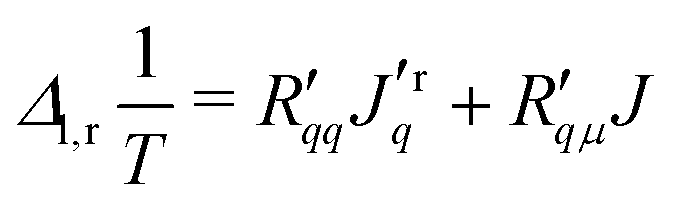
The flux equations in non-equilibrium thermodynamics are dictated by the entropy production. Their derivation from the entropy production will not be repeated, however. For details, see ref. 7 and 30. We present below two equivalent forms, practical for different purposes. The formulation using measurable fluxes and forces, and a matrix of conductance coefficients, can most easily be related to experiments. The formulation using a matrix of resistance coefficients can be more directly related to simulations. As the entropy production is invariant, one form can be transformed into the other. We shall make use of this property.As independent flux variables, we choose the molar flux, J, and the measurable heat flux, Jrq, on the right-hand side of the membrane. The two conjugate driving forces are then the difference in the inverse temperature, and minus the difference in the pressure difference over the constant temperature on the left-hand side.32 With a pure solvent on both sides, the only contribution to the chemical potential difference is the pressure difference. The driving force −VrmΔl,rp/Tl, must be evaluated at the temperature on the left-hand side, Tl, when the heat flux is measured on the right-hand side, see Kjelstrup and Bedeaux.32 This condition is not explicit in other descriptions.26
The flux-force relations of the membrane system are then
 | (1) |
 | (2) |
 are the conductance coefficients. They refer to transport between positions r and l.
By inverting eqn (1) and (2) we obtain the force–flux relations with the matrix of overall resistance coefficients,
 | (3) |
 | (4) |
The coefficient matrices are symmetric according to Onsager.32 The Onsager relations  apply, so only three coefficients need be determined in one set. The coefficients may depend on state variables, like temperature and pressure, but do not depend on the forces and fluxes. We can therefore use a particular set of forces to find a coefficient, but we can use the coefficient with other sets of forces. This is important here. As long as the relations of eqn (3) and (4) are linear, we can use special conditions to find a coefficient, but their application is general. Our aim is to find all coefficients central to thermal osmosis and conductance, as well as resistance coefficients.
 can be related to the Fourier conductivity, and
  to the water permeability.30 The coefficient
  is the Dufour coefficient, which can be related to thermal diffusion (see eqn (10) below). Eqn (1) reduces in the absence of the pressure gradient, i.e. for no gradient in chemical potential, to a form which can be related to the thermal conductivity:
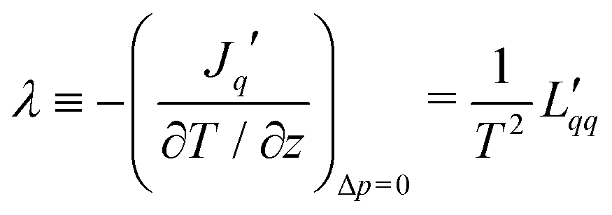 | (5) |
 | (6) |
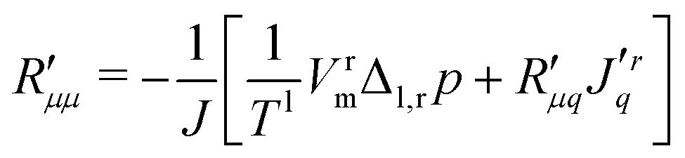
 -coefficients. The main resistance to heat transport is defined in the absence of a mass flux. A temperature difference is applied to the membrane, and the value of the heat flux is recorded when the mass flux stops (J = 0). We obtain from eqn (3)
 | (7) |
The coupling coefficient for mass and heat transfer is determined from eqn (4), also in the absence of a mass flux:
 | (8) |
When J = 0, there is balance between thermal and chemical forces. By analogy to cases of binary homogeneous mixtures, we may then speak of a Soret equilibrium state for fluid in a porous membrane. We may distinguish between two types of Soret equilibria. In the first case the temperature difference leads to a concentration difference. In the second case it leads to a pressure difference. In the first case we have thermal diffusion, and in the second case, we have thermal osmosis. A balance of forces (Soret equilibrium) can be reached in both cases. In the present case, the balance of forces gives the ratio of coefficients:
 | (9) |
 | (10) |
 and
and  . The main coefficient is given from eqn (4) when the heat flux is zero:
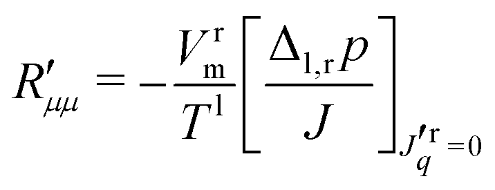 | (11) |
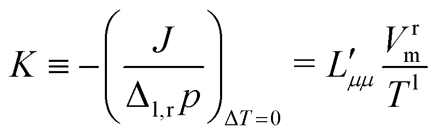
Knowledge of the coupling coefficient  from eqn (9) gives an alternative route to the main coefficient, viaeqn (4). The mass transfer resistance can be computed from any known pressure difference using
 | (12) |
 | (13) |
 | (14) |
 ;
; | (15) |
3 Molecular dynamics simulations
3.1 Interaction potential
The basics of non-equilibrium molecular dynamics (NEMD) are well described, see e.g.ref. 35. Reduced variables are used instead of real variables. Their connection can be found in ref. 36. For the conversion of reduced units to real units, we used values typical for water, i.e. a potential depth of ε/k = 741 K, a diameter of d0 = 3.25 × 10⁻¹⁰ m and a mass m = 2.99 × 10⁻²⁶ kg, which were obtained via the critical temperature Tc = 647.1 K and the critical pressure pc = 220 bar of water. In this sense, our model can be regarded as a coarse-grained water model. Simulations were carried out with fluid reservoirs of different temperatures connected by a pore of varying diameter and length. The temperatures were defined by means of the temperature in the bulk phases. The densities of the liquid reservoirs (hot and cold) were chosen after inspecting the phase diagram for the Lennard-Jones/spline potential in use.37 The simulation boxes were elongated in the z-direction and had side lengths Lx = Ly ≠ Lz, with periodic boundary conditions in all directions. The pores were constructed using a face-centered cubic crystal of immobilized particles and deleting particles within a cylindrical region. We used the averaged position of the first row of wall particles in the radial direction to the center of the pore, to determine the diameter of the pores. By immobilizing the particles, the wall was insulating (not conducting heat). The choice of a perfect isolating wall had the advantage of avoiding energy loss through the solid. This enabled us to compute transfer coefficients for well defined liquid reservoir conditions, which are needed for conceptual studies like this. It further enabled us to relate both fluxes (heat and mass) through the system to the same cross-sectional area of the pore.There was a negligible impact of the particles’ center of mass velocity on the computation of the temperature and pressure in the liquid phase. For the vapor phase, a systematic correction was needed due to shifts in the center of mass velocity. The correction was done using the steady-state center of mass velocity, averaged over time.
In all simulations, the interaction between particles of type i and j was defined by the Lennard-Jones/spline potential,37,38
 | (16) |
3.2 Pressure computation
The mechanical pressure was computed following Kirkwood:41 | (17) |
3.3 Case I: Soret equilibrium
To model a Soret equilibrium, we set up a symmetric system with two fluid reservoirs connected by a hydrophobic pore with periodic boundary conditions in all directions (see Fig. 3). The aspect ratio of the simulation box was 4.2 for the simulations of the short pore and 5 for simulations of the long pore. Different temperature gradients between the two reservoirs were established by thermostatting two layers in each reservoir. The isolating wall in combination with small pore sizes enabled us to avoid temperature polarization45 and maintain almost constant temperatures within the liquid reservoirs for all simulations of Case I. The liquid reservoirs temperatures were, within a deviation of less than 2%, equal to the temperatures of the two liquid–vapor interfaces. This set-up enabled a steady-state mass flux driven by the temperature difference between the hot and cold reservoirs. To investigate the effect of a pressure difference between the two reservoirs on the steady state mass flux, we used the reflecting particle boundary method (RPM) of Li et al.46 The RPM enabled us to gradually increase the pressure in the cold liquid reservoir while decreasing the pressure in the hot one. The mass flux stopped when the pressure in the cold liquid reservoir was so high that the thermal and mechanical forces reached a balance, the so-called Soret equilibrium. | ||
| Fig. 3 Set-up for simulation of the Soret equilibrium. The pore length is L = 6 nm. | ||
We made sure that the flow conditions were such that the pressure difference, caused by the temperature difference, was lower than the liquid entry pressure of the pores, i.e. that the fluid was only transported as a vapor.47 The temperatures of the reservoirs were controlled using a temperature rescaling algorithm. The temperature rescaling-thermostat was compared to a Langevin thermostat. Both types of thermostats gave the same mass flux. This remained so, independent of the pressure difference.
The steady-state mass flux as well as the total heat flux, or energy flux, were computed in the pore. In the absence of a mass flux, the total heat flux is equal to the measurable heat flux. In the presence of a mass flux, the measurable heat flux on the right-hand side (i.e. the cold reservoir),  , was obtained from the total heat flux minus the mass flux contribution, i.e.
 = Jq − JHr. The molar enthalpy was calculated in a separate simulation, as a function of the pressure and temperature.
The system was simulated for three pore diameters, dp = 1.7, 2.7, and 3.8 nm, and two pore lengths, L = 6 and 12 nm, for temperature differences in the range ΔT = 21.9–109.7 K.
By gradually changing the pressure difference between the liquid reservoirs, we obtained data for a set of fluxes, densities and pressures at a fixed temperature difference and pore geometry. We determined the coefficients by fitting eqn (3) and (4) to this data set using the least squares method. Each condition was simulated 5 times with 9.8 million time steps.
3.4 Case II: steady state mass flux
The steady state mass flux in the absence of a pressure difference was investigated for the three pore diameters used in Case I as well as for larger pores. The system size was increased and is shown in Fig. 4. The aspect ratio of the simulation box was 6.7. Pore diameters were dp = 1.7, 2.7, 3.8, 4.9, 6.1, 7.2, 8.3, 9.4, and 10.6 nm, and the pore length was L = 23.3 nm.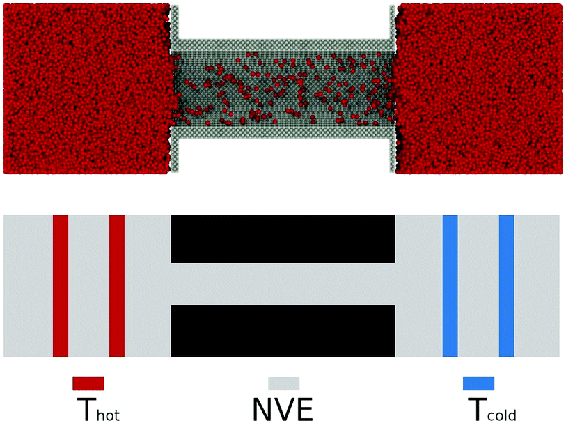 | ||
| Fig. 4 Set-up for simulation of a steady state mass flux in the absence of a pressure difference. Pore diameters were varied. | ||
The thermal reservoirs were again controlled by thermostatting two layers in each reservoir. We observed temperature polarization for the three largest pores simulated in Case II. This issue is discussed in the corresponding segment in Section 4. Simulations were carried out for different temperature differences between ΔT = 21.9 K and 138.9 K. Each condition was simulated 5 times with 980.000 time steps.
3.5 Cases studied
Coefficients were obtained for two cases.In Case I the system (see Fig. 3) was simulated for three pore diameters, dp = 1.7, 2.7, and 3.8 nm, and two pore lengths, L = 6 and 12 nm. The temperature differences varied from ΔT = 21.9–109.7 K.
In Case II, the system size was increased (see Fig. 4). Simulations were done for pore diameters dp = 1.7, 2.7, 3.8, 4.9, 6.1, 7.2, 8.3, 9.4, and 10.6 nm with a pore length L = 23.3 nm. The temperature differences varied from ΔT = 21.9 to 138.9 K.
4 Results and discussion
All results obtained from the equations above and corresponding molecular dynamics simulations are shown in Fig. 6–15. Fig. 5 shows some initial conditions. | ||
| Fig. 5 (a) Liquid leaking through the largest pore. (b) Wetting angle from the liquid–solid interactions, determined by a tangential fit to the surface of the droplet. | ||
 | ||
Fig. 6 Total resistivity coefficients (a)  and (b) and (b)  plotted as a function of the temperature of the hot side. plotted as a function of the temperature of the hot side. | ||
 | ||
| Fig. 7 Thermo-osmotic pressure difference due to a temperature difference (Soret equilibrium) for different pore diameters and lengths. | ||
 | ||
| Fig. 8 Isothermal heat of transfer, q*, plotted as a function of the temperature of the hot side for three pore diameters and two pore lengths. | ||
 | ||
| Fig. 9 Cross-section of the fluid at the Soret equilibrium for the highest achievable temperature difference for a pore length of L1 = 6 nm. The pore diameters and temperature differences are (a) ΔT = 109.7 K and dp = 1.7 nm, (b) ΔT = 51.2 K and dp = 2.7 nm and (c) ΔT = 21.9 K and dp = 3.8 nm. | ||
 | ||
Fig. 10 Resistances to mass transfer ((a and b)) as well as the ratio of both resistances ((c)) plotted as a function of the temperature of the hot side. (a) The minimum obtainable resistance to mass transfer was computed viaeqn (14). (b) Actual resistance to mass transfer. (c) Ratio of theoretical minimum mass transfer resistance,  , and the actual resistance, , and the actual resistance,  . . | ||
 | ||
| Fig. 11 Mass flux plotted as a function of the pressure difference for dp = 2.4 nm and a pore length of L2 = 12 nm. The temperature difference was held constant at the respective highest used temperature difference of ΔT = 51.2 K. | ||
 | ||
| Fig. 12 (a) Pressure profiles along the system for the three mass fluxes marked with a circle with the corresponding color in Fig. 11. (b) Close up of the vapor pressure inside the right pore, as indicated by the dotted rectangle in (a). | ||
 | ||
| Fig. 13 (a) Mass flux plotted as a function of the pore diameter and (b) mass flux as a function of the temperature difference. | ||
 | ||
| Fig. 14 (a) Temperature profile and (b) pressure profile along the system for a pore of diameter dp = 8.3 nm and varying temperature differences. | ||
 | ||
Fig. 15 Total conductivity coefficients (a)  , (b) , (b)  and (c) and (c)  plotted as a function of the temperature of the hot side. plotted as a function of the temperature of the hot side. | ||
4.1 Upper pressure limit: the liquid entry pressure
The liquid entry pressure is defined as the pressure observed when liquid starts to leak back through the membrane and is in general determined for a dry membrane.47,48 The leak will take place when the pressure in the liquid reservoir becomes too high for the membrane to sustain. As a consequence, the liquid pushes through the pore (see Fig. 5(a)).To establish a range of working pressures, we first considered the limit given by the liquid entry pressure and ensured for every simulation that liquid was only transported in the vapor phase. A control for each simulation was necessary as the liquid entry pressure might change with varying conditions inside the pore/membrane. Leakage was observed by inspecting pore snapshots as well as the pressure profile along the system for the two largest pore diameters investigated. For pores with diameter dp = 2.7 nm and dp = 3.8 nm, we obtained Pcold ≈ 1034 bar and Tcold = 468 K, and Pcold ≈ 548 bar and Tcold = 483 K, respectively. These liquid entry pressures, as defined by the total pressure of the liquid bulk phase on the cold side, are then upper limits for the thermo-osmotic pressures of the pore diameter in question. The liquid entry pressure is a mechanical property of the porous membrane, and has no impact on the transport properties, unless it deforms the membrane. The high liquid entry pressures obtained here indicate that our artificial membrane is rather strong. For this conceptual study of the Soret equilibrium, it was important not to be limited by the material properties, i.e. the solid. Immobilizing the wall particles had thus not only the advantage of limiting energy loss through the system but also obtaining pressures independent of the mechanical strength of the membrane. It is well known that the liquid entry pressure depends on the cross-sectional area of the pore, the liquid–solid surface tension as well as the conditions of the liquid reservoir.47 We determined the wetting angle by a simple tangential fit to the surface of a droplet on the used wall material, see Fig. 5(b). The wetting angle was found to be θ = 125° ± 6°, which is comparable to water on a polyvinylidene fluoride membrane.49 The value is in the range of the current limits for contact angles of water on a smooth surface.50 The high contact angle was obtained by tuning the α-parameter for the fluid–solid interaction of the potential in use. This had the advantage that a high liquid entry pressure could be obtained without the introduction of a rough surface.
By running non-equilibrium molecular simulations, it is often necessary to use temperatures, pressures, gradients as well as time scales that differ from experimental setups, in order to obtain good statistics with a reasonable simulation time. While it might not be possible to experimentally maintain the conditions used in the present study, i.e. the high liquid entry pressure as well as the applied temperature gradients, the properties remain the same as long as there is a linear response. Within a linear response regime, it is possible to determine the properties and link them to a system with more realistic boundary conditions. One such approach is given by Wilhelmsen et al., who used the square-gradient theory in order to link experimental evaporation results to those obtained from non-equilibrium molecular simulations.31
The results below were obtained for pressures below the limit given by the liquid entry pressure.
4.2 Resistances to heat transfer. Thermo-osmotic pressure
The resistances and
and  are shown in Fig. 6(a) and (b). They are plotted as a function of the left-hand side temperature (hot side temperature) to test for a possible temperature dependence, which was reported to be significant for transport across liquid–vapor interfaces.31 The results are scattered, mainly due to fluctuations in the heat flux; in particular for smaller temperature differences, but a dependence on the temperature cannot be reported. Within the accuracy of the computed property there is no such variation within the range of temperatures applied, i.e. of 50 K.
Fig. 6(a) and (b) show that the two resistances to heat transfer depend somewhat on the pore length and diameter. Again, the results are scattered, but a systematic tendency can be observed for  , where the longest pore has the highest resistance. On average, by doubling the pore length from 6 to 12 nm, we increased
  by a factor 1.4. An increase of resistance can be expected, since the contribution of the pore to the overall resistance increases with increasing pore length. However, due to the contributions from the two interfaces at the entrance to the pore, the resistance does not double for the long pore. The water model in use exhibits a lower surface tension compared to the one of real water at the given temperatures. One may therefore expect that the contribution of the two interfaces increases for real water. The variation in the coefficients seen with the pore diameter is, however, not so easy to explain. Within the accuracy of the simulations, the resistance appears to decrease with increasing pore radius.
The meaning of the coupling coefficient  becomes more clear when we observe conditions for the Soret equilibrium. Fig. 7 shows the observed pressure difference caused by a temperature difference, at the point when the Soret equilibrium has been reached. We report results for three different pore diameters and two pore lengths. All points fall on one line. The thermo-osmotic pressure of the membrane is expressed by the slope of this line, s = −18 bar K−1. This is in the range of values found for the thermo-osmotic pressure in frost heave, where an ice lens is growing against a pressure by supply of sub-cooled water.51
The Soret equilibrium state is clearly only a function of the applied temperature difference and, in the present case, not of the pore diameter or pore length. The independence of s on the pore length is expected. This follows from eqn (10), where the geometrical contributions cancel out. We can use this coefficient to characterize the membrane′s ability to produce the thermo-osmotic effect.
The isothermal heat of transfer, q*, was computed in two ways: from the ratio of  and
and  in Fig. 6, and from the ratio of ΔP and ΔT in Fig. 7. The results are shown in Fig. 8 as a function of the temperature of the hot side. These results also fall on the same line. The ratio of coefficients is much less scattered than was seen for single coefficients. This is because the measurable heat flux cancels out in the ratio. The ratio of
  and
and  , or the reversible heat of transfer, q*, is remarkably constant. The dependence on geometric variables, seen in the single coefficients, has disappeared, as is also expected. The sign of the heat of transfer arises from the coupling coefficient,
  . It is positive in the present system, cf.eqn (8). Heat transport is thus enhanced by mass transport, or vice versa; mass transport is enhanced by heat transport. Apart from kinetic theory, few models for the heat of transfer exist that address interface transport. Kjelstrup and Bedeaux32 showed that the heat of transfer for evaporation was a fraction of the enthalpy of the phase transition. The average value for q* in our primitive water model is 23.5 kJ mol−1. The evaporation enthalpy of a flat liquid–vapor interface, as computed in a separate simulation for the average temperature (T = 483.5 K), was found to be ΔvapH = 25 kJ mol−1. This is smaller than the evaporation enthalpy of real water at the same reference temperature (33.3 kJ mol−1) and is caused by the simplicity of our water model. Reasoning from this, we may expect that the positive sign of q* originates from the evaporation and condensation in the vicinity of hydrophobic interactions of fluid–wall particles, as the interaction between the membrane and the fluid determines the sign of the heat of transfer.26 This sign is essential for where the pressure builds. A positive isothermal heat of transfer will create a high pressure on the low-temperature side, whereas a negative q* creates a high pressure on the high-temperature side. For the MemPower process only the first case is useful.
To obtain more insight into the contributing mechanisms, we studied pore snapshots under various conditions, see Fig. 9. This figure shows, for each pore diameter with a pore length L = 6 nm, the conditions at the Soret equilibrium for the highest achievable temperature difference. The high pressure developed on the cold side at the Soret equilibrium pushes fluid into the pore and creates a curved surface between the liquid and the vapor phase. It is thus conceivable that curvature and/or confinement effects within the pore might have an impact on the single coefficient determinations. Another effect that might contribute to the overall transport coefficients is the so called thermal creep, which is a fluid flow induced by a gradient in temperature along the wall.52 Such an effect was not present in the given system due to the immobilization of the wall particles. Immobilization was used to avoid energy loss through the solid and to reduce the effect of temperature polarization within the two liquid reservoirs.
4.3 Minimum and actual resistance to mass transfer
The theoretical minimum resistance to mass transfer, , as computed from eqn (14), is shown for various pore diameters and two pore lengths in Fig. 10(a) as a function of the temperature of the hot side. The minimum resistance to mass transfer increases on average with a longer pore length and shows similar behaviour to
  and
and  . Again, the behaviour seen for longer pores is expected. The actual resistance to mass transfer,
  , for the same conditions is shown in Fig. 10(b). All values are larger than the theoretical minimum-values in Fig. 10(a). This follows from eqn (13).
The difference between  and
and  decreases on average with increasing pore diameter. Due to the fluctuations in the fluxes, the coefficients of the real resistance to mass transfer are scattered. However, on average, also here the resistance is increasing with a longer pore and a smaller pore diameter.
The ratio of the theoretical minimum,  , and the actual minimum,
  , is shown in Fig. 10(c) as a function of the temperature of the hot side. With increasing pore diameter, the difference between both decreases. This ratio is interesting, as it implies (following eqn (13)) that the coupling coefficients have the same order of magnitude as the main coefficients. The coupling effects are large, in other words. Large coupling effects are beneficial for work to be done, like here. Clearly, this hydrophobic membrane is beneficial for the effect we want, to generate a pressure difference.
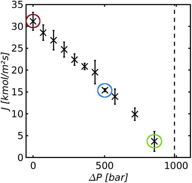
Fig. 11 shows the mass flux plotted as a function of the pressure difference for a pore with a diameter dp = 2.4 nm and a length L = 12 nm. The temperature difference was held constant at ΔT = 51.2 K.
The mass flux decreases linearly with increasing pressure difference and approaches zero as the pressure difference approached its value in Soret equilibrium (marked by the dashed line). The linear relation between the mass flux and the pressure follows from eqn (4). The slope of Fig. 11 gives the the permeability K = −(Jm/Δp) = 3.1 × 10⁻⁵ mol (m2 s Pa)−1. The permeability is of the same order of magnitude as values reported in the literature.53
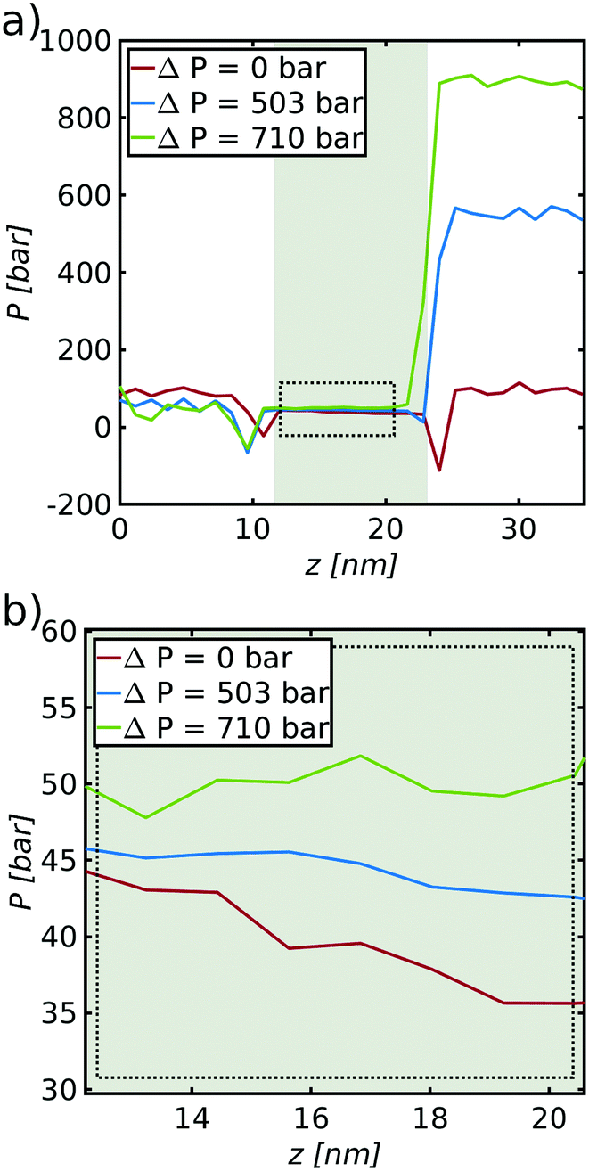
We return to the issue of pressure profiles, to be able to discuss the role of the vapor pressure on the transport of mass; in particular how a variation in this pressure with temperature plays a role for the mass transport. Pressure profiles along the system are shown in Fig. 12(a) for the three mass fluxes, marked with a circle with the corresponding color in Fig. 11.
The curves on the right reflect properties of the cold liquid reservoir. The values on the left reflect properties of the hot reservoir, shown here by a white background color. The reservoirs are connected by the hydrophobic pores filled with vapor (the gray background color). The pressure of the cold liquid reservoir increases, while the pressure of the hot liquid reservoir decreases. The dips at the two entrances of the pore indicate surfaces under tension.54 A close up of the vapor pressure inside the pore, as indicated by a dotted rectangle, is shown in Fig. 12(b).
We observe that the pressure of the vapor inside the pore flattens out with increasing pressure difference (decreasing mass flux) between the hot and cold liquid reservoirs.
In the non-equilibrium situation (in the presence of a mass flux) the vapor pressure in the pore is not the pressure of the equilibrium vapor pressure for the liquid at the temperature in question. The pressure gradients seen in the picture are sustained by the mass flux. The lack of a gradient in the Soret equilibrium can be understood from the system's lack of ability to sustain a pressure gradient inside the vapor phase in this case (J ≈ 0). The vapor pressure gradient does not play a role for the balance of forces in the Soret equilibrium.
Rauter et al. showed that all interactions with the surface must be included to find the correct pressure for equilibrium conditions in slit nano-pores.39 The given geometry and pressure computation did not enable us to do so. We ran similar simulations for a slit pore to compare our findings. While the total value of the two tangential components (including all interactions with the solid surface) shifted to a lower level compared to the bulk phase in the center, the gradient did not change recognizably. We expect therefore that for the given geometry the gradient remains the same, independent of an inclusion of the interactions with the solid. This is reasonable as our pore has no gradient in surface tension and the vapor particles have reduced contact with the wall, such that an impact of the local temperature on the fluid–solid interaction is likely to be negligible.
The fact that the pressure gradient disappears inside the pore is not surprising, as there is no possible way that a pressure gradient can be sustained in the vapor-filled pore when there is no mass flux. Thus, the thermo-osmotic pressure (the Soret equilibrium) is not sustained through a gradient in vapor pressure, but only by pressure jumps at the two liquid–vapor surfaces, in particular at the cold side. The results provide a numerical argument to the discussion about the vapor pressure gradient as a potential independent driving force of transport for the fluid from one side of the membrane to the other. There can still be a gradient in vapor pressure due to temperature variations, but any gradient in this pressure is a secondary effect, not a primary cause of transport. While it might be possible to explain local transport effects via the local vapor pressure, it can not be used for an overall description of the system. This is contrary to what has been reported in the literature, where the vapor pressure difference has been designated as the driving force,25 and appears to be important for further modelling.
4.4 The thermal driving force
To understand better the effect of the thermal driving force under isobaric conditions and what that may mean in practice, we simulated steady state mass transport with pore diameters in the range from dp = 1.7 to dp = 10.6 nm for temperature differences between ΔT = 21.9 and ΔT = 138.9 K. The pore length was L = 23.3 nm. The results are shown in Fig. 13 and 14.Fig. 13(a) and (b) show the thermo-osmotic flux as a function of the pore diameter and temperature difference, respectively, under isobaric conditions. The mass flux is here dependent on the pore size for the simulated pore diameters. The mass flux increases with increasing pore diameter up to a diameter of dp = 4.9 nm and then remains constant. The mass flux scales linearly with the applied temperature difference for all pore diameters.
The local mass transfer mechanisms of vapor inside a hydrophobic membrane are generally described by Knudsen flow, transition flow and an ordinary diffusion regime.55 It has also been shown that not only the pore diameter has an impact on the mass transport, but also the size of the evaporation area.12 In our model, the evaporation area is directly related to the cross-section of the pore, such that both effects, i.e. a change of flow regime as well as the evaporation itself, might cause a decreasing mass flux for pore diameters smaller than 4.9 nm. A more detailed investigation will follow in future work.
The relationship between the molar flux, J, and the applied temperature difference, ΔT, gives the thermo-osmotic coefficient. The thermo-osmotic coefficient is (DT)Δp=0 = JL/ΔT = 2.3 × 10⁻⁵ mol (m s K)−1 and (DT)Δp=0 = 2.7 × 10⁻⁶ mol (m s K)−1 for the largest and smallest pore, respectively. While the smallest pore is approximately two times smaller than the highest value reported in the literature, the largest pore exceeds this value by around 5 times.14 It is promising that we find such a high value for the largest pore. This is however not surprising, because our simulation study is carried out for a single straight pore, while a real porous membrane has often a distribution of pore sizes and tortuosity factors, which both have an impact on the overall thermo-osmotic coefficient.
A large pore diameter may be preferable from a manufacturing point of view, while a small diameter may be preferable from the perspective of membrane strength and cost per membrane area. The last-mentioned membrane may sustain a higher thermo-osmotic pressure because it has a higher liquid-entry pressure.
The temperature and pressure profiles along the system are shown for five different temperature differences for the pore with a diameter dp = 8.3 nm in Fig. 14(a) and (b), respectively. On the left-hand side is the hot liquid reservoir and on the right-hand side is the cold one. The pore extends approximately from 18.0 to 41.0 nm – this is indicated by the gray background color in both figures. With an increasing temperature difference between the hot and the cold reservoir, the temperature gradient across the system must also increase. We observed increasing temperature gradients in the liquid reservoirs for the three largest pores. The effect of temperature polarization, a common issue reported in ref. 45, did not lead to a recognisable decrease in mass flux. There is no difference in pressure between the two liquid reservoirs for all temperature differences.
However, in all these cases there is a non-negligible gradient in pressure inside the pore, see Fig. 14(b). The pressure in the pore is the fluid vapor pressure. We see a small but noticeable increase with the increasing local temperature, meaning that the vapor pressure will increase correspondingly as there is local equilibrium along the path. The figure shows that the higher the temperature is, on the hot side, the larger is the pressure gradient in the pore. The variation is pointing in the direction of mass transport, but again, we know that the vapor pressure is not an independent variable. Two independent fluxes and forces describe our coupled transport of heat and mass. These are defined by the boundaries of Fig. 2. Any deviation in the vapor pressure from the equilibrium vapor pressure, may, however occur, and may contribute to the single interface-process across interfaces 1 and 3 in Fig. 2. But these contributions will be embedded in an overall black-box-like description, and deserve a separate study.
The coefficients of the  -matrix are derived from the criterion of entropy production invariance and obey the criteria specified in Section 2.
5 Conclusions and perspectives
We have investigated the non-equilibrium thermodynamic concepts for transport of fluid against a pressure through a vapor-gap membrane, namely the fluxes and forces deriving from the entropy production, along with their coupling. These concepts are relevant for water cleaning and power production purposes. Here, only a coarse-grained model was used. Repulsive wall–particle interactions were used to mimic hydrophobic interactions between water and a membrane wall. Such a potential is the first essential requirement for the process to work. With this requirement in place, we have.• demonstrated that a Soret equilibrium exists across a membrane pore. The thermo-osmotic pressure was 18 bar K−1.
• found that the Soret equilibrium cannot be be sustained by a variation in the fluid vapor pressure.
• obtained a heat of transfer of 23.5 kJ mol−1 which was nearly constant for a range of pore lengths and diameters. A positive heat of transfer is required to transport water against a pressure difference. The heat of transfer is a fraction (∼0.9) of the evaporation enthalpy of a flat liquid–vapor interface, which was ΔvapH = 25 kJ mol−1.
• derived a minimum value for the mass transfer resistance. This minimum value might be interesting for membrane design.
• found that the overall resistance to mass transfer was close to the value of the minimum resistance to mass transfer, in this hydrophobic membrane.
• experienced that the precise shape and property of the liquid–vapor interface may have an important influence on the transport coefficients.
These results apply to the coarse-grained water model used here, but there are good reasons to believe that the concepts proven and the method of analysis may be useful for the design of water cleaning and power production technologies for other membranes and water solutions, as in the MemPower unit.6
Author contributions
M. R. wrote software and carried out the calculations. M. R., S. K. S., B. H. and S. K. contributed to the conceptual design and development. The project was supervised by S. K. S. and S. K. All authors contributed to the writing of the manuscript and the scientific discussions. All authors have read and agree to the published version of the manuscript.Funding
This research was funded by the Center of Excellence funding scheme of the Research Council of Norway, project no. 262644, PoreLab.Conflicts of interest
The authors declare no conflict of interest.Acknowledgements
The authors greatly appreciate discussions with Dick Bedeaux and Laura Edvardsen. Thanks to the Research Council of Norway through its Centres of Excellence funding scheme, project number 262644, PoreLab. SKS acknowledges funding through the Research Council of Norway and the Young Research Talents Scheme with project number 275754. The computational resources were granted by Sigma2 through NN9414K.Notes and references
- W. U. W. W. A. Programme, The United Nations World Water Development Report 2019: Leaving No One Behind, 2019.
- S. M. Salman, Water Int., 2005, 30, 415–418 CrossRef.
- M. Muller, Civ. Eng. = Siviele Ingenieurswese, 2017, 2017(5), 11–16 Search PubMed.
- M. Qasim, M. Badrelzaman, N. N. Darwish, N. A. Darwish and N. Hilal, Desalination, 2019, 459, 59–104 CrossRef CAS.
- Y. Ghalavand, M. S. Hatamipour and A. Rahimi, Desalin. Water Treat., 2015, 54, 1526–1541 CAS.
- N. Kuipers, J. H. Hanemaaijer, H. Brouwer, J. van Medevoort, A. Jansen, F. Altena, P. van der Vleuten and H. Bak, Desalin. Water Treat., 2015, 55, 2766–2776 CrossRef CAS.
- L. Keulen, L. Van Der Ham, N. Kuipers, J. Hanemaaijer, T. Vlugt and S. Kjelstrup, J. Membr. Sci., 2017, 524, 151–162 CrossRef CAS.
- A. P. Straub, N. Y. Yip, S. Lin, J. Lee and M. Elimelech, Nat. Energy, 2016, 1, 16090 CrossRef CAS.
- G. Meindersma, C. Guijt and A. De Haan, Desalination, 2006, 187, 291–301 CrossRef CAS.
- L. Camacho, L. Dumée, J. Zhang, J.-d. Li, M. Duke, J. Gomez and S. Gray, et al. , Water, 2013, 5, 94–196 CrossRef.
- J. P. Villaluenga and S. Kjelstrup, J. Non-Equilib. Thermodyn., 2012, 37(4), 353–376 Search PubMed.
- J. Liu, Q. Wang, H. Shan, H. Guo and B. Li, J. Membr. Sci., 2019, 580, 275–288 CrossRef CAS.
- A. Jansen, J. Assink, J. Hanemaaijer, J. Van Medevoort and E. Van Sonsbeek, Desalination, 2013, 323, 55–65 CrossRef CAS.
- V. M. Barragán and S. Kjelstrup, J. Non-Equilib. Thermodyn., 2017, 42, 217–236 Search PubMed.
- R. Srivastava and P. Avasthi, J. Hydrol., 1975, 24, 111–120 CrossRef.
- L. Fu, S. Merabia and L. Joly, J. Phys. Chem. Lett., 2018, 9, 2086–2092 CrossRef CAS PubMed.
- K. Zhao and H. Wu, Nano Lett., 2015, 15, 3664–3668 CrossRef CAS PubMed.
- M. R. Chowdhury and J. R. McCutcheon, J. Membr. Sci., 2018, 553, 189–199 CrossRef CAS.
- K. Touati, C. Hänel, F. Tadeo and T. Schiestel, Desalination, 2015, 365, 182–195 CrossRef CAS.
- S. Kim and M. Mench, J. Membr. Sci., 2009, 328, 113–120 CrossRef CAS.
- I. Wold and B. Hafskjold, Int. J. Thermophys., 1999, 20, 847–856 CrossRef CAS.
- D. Tracy, J. Phys. E: Sci. Instrum., 1974, 7, 533 CrossRef CAS.
- J. Lee, T. Laoui and R. Karnik, Nat. Nanotechnol., 2014, 9, 317 CrossRef CAS PubMed.
- K. Park, D. Y. Kim and D. R. Yang, Ind. Eng. Chem. Res., 2017, 56, 14888–14901 CrossRef CAS.
- M. Qtaishat, T. Matsuura, B. Kruczek and M. Khayet, Desalination, 2008, 219, 272–292 CrossRef CAS.
- X. Liu, L. Shu and S. Jin, J. Membr. Sci., 2019, 580, 143–153 CrossRef CAS.
- J. K. Platten, J. Appl. Mech., 2006, 73(1), 5–15 CrossRef CAS.
- L. van der Ham and S. Kjelstrup, Int. J. Thermodyn., 2011, 14, 179–184 CAS.
- P. Jafari, A. Masoudi, P. Irajizad, M. Nazari, V. Kashyap, B. Eslami and H. Ghasemi, Langmuir, 2018, 34, 11676–11684 CrossRef CAS PubMed.
- S. Kjelstrup, D. Bedeaux, E. Johannessen and J. Gross, Non-equilibrium thermodynamics for engineers, World Scientific, Singapore, 2nd edn, 2017 Search PubMed.
- Ø. Wilhelmsen, T. T. Trinh, A. Lervik, V. K. Badam, S. Kjelstrup and D. Bedeaux, Phys. Rev. E, 2016, 93, 032801 CrossRef PubMed.
- S. Kjelstrup and D. Bedeaux, Non-equilibrium thermodynamics of heterogeneous systems, Series on Advances in Statistical Mechanics, World Scientific, Singapore, 2nd edn, 2020, vol. 20 Search PubMed.
- F. Bonetto, J. L. Lebowitz and L. Rey-Bellet, Math. Phys. 2000, World Scientific, 2000, pp. 128–150 Search PubMed.
- S. Whitaker, Transp. Porous Media, 1986, 1, 3–25 CrossRef.
- G. Arya, H.-C. Chang and E. J. Maginn, J. Chem. Phys., 2001, 115, 8112–8124 CrossRef CAS.
- B. Hafskjold, T. Ikeshoji and S. K. Ratkje, Mol. Phys., 1993, 80, 1389–1412 CrossRef CAS.
- B. Hafskjold, K. P. Travis, A. B. Hass, M. Hammer, A. Aasen and Ø. Wilhelmsen, Mol. Phys., 2019, 1–16 CAS.
- D. Frenkel and B. Smit, Understanding molecular simulation: from algorithms to applications, Elsevier, Amsterdam, 2nd edn, 2001, vol. 1 Search PubMed.
- M. T. Rauter, O. Galteland, M. Erdös, O. A. Moultos, T. J. Vlugt, S. K. Schnell, D. Bedeaux and S. Kjelstrup, Nanomaterials, 2020, 10, 608 CrossRef CAS PubMed.
- S. Plimpton, J. Comput. Phys., 1995, 117, 1–19 CrossRef CAS.
- J. G. Kirkwood and F. P. Buff, J. Chem. Phys., 1949, 17, 338–343 CrossRef CAS.
- B. Hafskjold and T. Ikeshoji, Phys. Rev. E: Stat., Nonlinear, Soft Matter Phys., 2002, 66, 011203 CrossRef PubMed.
- T. Ikeshoji, B. Hafskjold and H. Furuholt, Mol. Simul., 2003, 29, 101–109 CrossRef CAS.
- B. Todd, D. J. Evans and P. J. Daivis, Phys. Rev. E: Stat. Phys., Plasmas, Fluids, Relat. Interdiscip. Top., 1995, 52, 1627 CrossRef CAS PubMed.
- L. Martnez-Dez and M. I. Vazquez-Gonzalez, J. Membr. Sci., 1999, 156, 265–273 CrossRef.
- J. Li, D. Liao and S. Yip, Phys. Rev. E: Stat., Nonlinear, Soft Matter Phys., 1998, 57, 7259 CrossRef CAS.
- M. d. C. Garca-Payo, M. A. Izquierdo-Gil and C. Fernández-Pineda, J. Colloid Interface Sci., 2000, 230, 420–431 CrossRef PubMed.
- K. Smolders and A. Franken, Desalination, 1989, 72, 249–262 CrossRef CAS.
- X. Lu, Y. Peng, L. Ge, R. Lin, Z. Zhu and S. Liu, J. Membr. Sci., 2016, 505, 61–69 CrossRef CAS.
- J. Wang, Y. Wu, Y. Cao, G. Li and Y. Liao, Colloid Polym. Sci., 2020, 298, 1107–1112 CrossRef CAS.
- S. Ratkje, H. Yamamoto, T. Takashi, T. Ohrai and J. Okamoto, CRREL, 1982, 131–135 Search PubMed.
- K. Aoki, P. Degond and L. Mieussens, Commun. Comput. Phys., 2009, 6, 919 CrossRef.
- A. Alkhudhiri, N. Darwish and N. Hilal, Desalination, 2012, 287, 2–18 CrossRef CAS.
- C. K. Addington, Y. Long and K. E. Gubbins, J. Chem. Phys., 2018, 149, 084109 CrossRef PubMed.
- M. Khayet, Adv. Colloid Interface Sci., 2011, 164, 56–88 CrossRef CAS PubMed.
| This journal is © the Owner Societies 2021 |