Morphology, energetics and growth kinetics of diphenylalanine fibres

Abstract

Diphenylalanine (FF) has been shown to self-assemble from water into heterogeneous fibres that are among the stiffest biomaterials known. How and why the fibres form has, however, not been clear. In this work, the nucleation and growth of FF fibres was investigated in a combined experimental and theoretical study. Scanning electron microscopy and optical microscopy showed FF fibre morphology to be hollow tubes of varying widths with occasional endcaps. Molecular dynamics simulations of FF nanostructures based on the bulk crystalline geometry demonstrated that axial growth stablilises the fibres and that structures with different widths show similar stabilities, in accord with the wide range of fibre widths observed experimentally. Linear dichroism (LD) spectroscopy was used to determine the thermal stability of the fibres, showing that FF solutions are fully monomeric at 70 °C and that fibres begin to form at ∼40 °C upon cooling. The LD kinetic studies indicated a nucleation-driven assembly with subsequent fibre growth, but a secondary nucleation process is required to explain the data.

---

Introduction

Peptides represent a unique group of functional biomolecules that can be used to create a variety of nanostructures. They are inherently biocompatible, with tuneable functionalities and often readily self-assemble. Structures that have been created include fibres, ribbons, micelles and vesicles.^2–8 Dipeptides are the smallest possible units and hydrophobic dipeptide assemblies have been well studied. As a general rule, peptide fibres are formed by linear peptide chains that are stacked perpendicular to the long axis of the fibre with hydrogen bonds parallel to the fibre axis stabilising the fibre. Extended structures are formed by lateral associations.

Recent work by Thacker et al.⁹ explored the role of hydrophobic interactions in the multiplication and propagation of peptide aggregates (or assemblies). The authors explored the concept of the primary nucleation (of monomeric amyloid-β, Aβ, peptides) to produce surfaces that catalyse the formation of fibres by monomers joining pre-existing aggregates. Thacker et al. focus is on the residues either side of the Aβ diphenylalanine (FF) which are on the surface of a fibril facilitating assembly of higher order aggregates whereas the FFs contribute to the assembly of the fibril. Their observed aggregation curves have a sigmoidal appearance, comprising a lag phase, an exponential phase, and a final plateau, characteristic of nucleated polymerisation reactions. Their kinetic modelling required primary nucleation, elongation, and what they refer to as surface-catalysed secondary nucleation.

Reches and Gazit discovered that FF dissolved in hexafluoroisopropanol (HFIP) and assembled into amyloid fibres when diluted with water.^10,11 They were then able to cast the fibres into metal nano wires. Ishikawa et al.¹² used Raman spectroscopy to study the initial stages of FF assembly into what they refer to a micro/nanotubes. They observed a change from monomeric FF to a structure they suggest is composed of 2–5 FF's over 1 s, followed by the formation of micro/nanotubes by 8–10 s after which no spectra change was observed on the timescale of their experiments. Görbitz found that FF has an unusual crystal structure when compared with other hydrophobic dipeptide assemblies, revealing a remarkable 3D π-stacked network with cylindrical hydrophilic pores of 1 nm in diameter which are parallel and aligned with the long axis of the fibre.^13,14 This work also showed that, contrary to what had been previously been thought, the fibres were large and had a wide range of sizes.¹⁴ Song et al. made important progress by preparing a hot solution of FF in water at 65 °C and then cooling it, leading to fibres forming.¹ This eliminates the requirement for an expensive, toxic, fluorinated solvent such as HFIP.

FF fibres are among the stiffest biomaterials known, with a Young's modulus of 27 GPa.¹⁵ This is similar to that of cortical bone, which has a Young's modulus ranging from 7 to 30 GPa.¹⁶ They also show notable chemical and thermal stability.¹⁷ Since their discovery, there has been a variety of work studying the properties of FF fibres as well as their applications. For example, modified fibres have been used to improve the performance of electrodes for enzyme-biosensor applications.¹⁸ FF fibres are piezoelectric and Krylov et al. have demonstrated piezoelectrically driven mechanical resonators based on them.¹⁹

However, despite the applications developed for FF fibres, very little is currently known about their formation process, which means that rationally tuning them for future applications is not currently possible. Some theoretical work suggests that small oligomers first associate by hydrophobic interactions between side chains and then electrostatic interactions steer the peptide backbones into an ordered state.²⁰ There have also been suggestions that the peptides first assemble into a sheet and then curl up into a tube.¹¹ Attempts in the literature to follow the self-assembly of FF into fibres by molecular dynamics (MD) simulations have been unsuccessful due to the very large systems needed, and the long timescale of self-assembly.^21,22 On the other hand, coarse graining has not replicated structures formed in experiments.²³ For example, Song's Monte Carlo simulations of coarse-grained FF molecules, showed FF behaving like a surfactant, assembling into unilamellar tubes or vesicles, which do not resemble the observed fibre structure.¹

The self-assembly of other amyloid disease-related proteins and peptides has been studied successfully. Xue et al. monitored the self-assembly of β2-microglobulin, which is a protein that can assemble into amyloid deposits in joints, and is found in dialysis-related amyloidosis.²⁴ They concluded that nucleation is the primary process for the assembly of the protein into fibrils which is followed by fragmentation of fibril that go on to seed further fibril growth. They suggest that this mechanism may be applicable to other amyloid systems. Indeed, it has been shown by Cohen et al.²⁵ that this nucleation and fragmentation mechanism applies also to Aβ, the Alzheimer's-related polypeptide which has FF as its central recognition motif.

The reason for the lack of understanding of FF fibre assembly is in part due to the difficulties faced when working with this system. The fibres have proved to be heterogeneous, which means that relying solely on a bulk technique which averages over many fibres is not adequate. Also, the phenylalanine chromophore has particularly weak absorbance signals in the near UV relative to other aromatic amino acids.²⁶ Further, the fibres’ shape is not spherical so, when using techniques involving light scattering, the interpretation of the data is challenging. In this work we have integrated experiment and modelling to characterise the assembly of FF fibres in a quantitative way, using spectroscopic kinetics experiments, microscopy and molecular dynamics simulations. Electron and optical microscopy allow us to observe the range of sizes the fibres span at different stages of assembly. Atomistic molecular dynamics simulations of relatively small FF assemblies give an insight into the reasons for the high aspect ratio exhibited by the fibres. Linear dichroism (LD), a spectroscopic technique which that has been shown to be a valuable tool for investigating the kinetics of fibre formation,^27–29 has been used to monitor the assembly of the FF fibres and their thermal stability. Our motivation throughout has been that it is important to understand the assembly of the elongated FF fibres in order to be able to control it for the variety of applications that have been proposed.

Materials and methods

FF was obtained from Sigma-Aldrich and used without further purification. For every experiment, a 2 mg mL⁻¹ solution of FF in deionised water was used. Fibres were grown according to the method described by Song et al.¹ They found 2 mg mL⁻¹ was required to ensure fibres rather than a mixture of fibres and vesicles form.

Scanning electron microscopy

FF was suspended in water at 70 °C for 1 hour. This solution was left to cool at room temperature overnight and then 10 μL were deposited onto a silicon substrate with a pipette. The solvent was left to evaporate in a fume hood until it was completely dry. This was coated in carbon by sputter coating before being put into a Zeiss SUPRA 55VP field emission gun scanning electron microscope (SEM). Fibre diameters were measured with ImageJ software from the SEM images. Other SEM samples were extracted from kinetic experiments.

Molecular dynamics

The FF crystal structure was obtained from the Cambridge Structural Database.³⁰ Atomistic simulations were performed using the CHARMM27 force field, including TIP3P for water. Calculations were implemented with NAMD and used the NVT ensemble with a Langevin heat bath, with a 1 fs timestep. Initial structures were built using Chimera,^31–33 and contained 54–750 FF molecules and of the order of 8,000 TIP3P water molecules in a simulation box of size 5.4 × 6.9 × 11.9 nm³. All simulations were conducted at 300 K. The root-mean-square deviation (RMSD) of the atomic positions of all FF molecules from their initial configuration was calculated as a function of time and was minimised through a rotation and translation fit; the resulting value was used as a measure of the stability of the structures (see ESI†).

The CHARMM27 force field is designed for simulating proteins and peptides and contains within it parameters for the naturally occurring amino acids. To test that it provided an accurate description of the FF system, an infinite crystal was first simulated. The simulation cell had periodic boundary conditions in three dimensions in a parallelepiped shape and the simulation was run for 0.4 ns with a 0.5 fs time step. An NPT (constant number, pressure and temperature) ensemble was used with a Nosé–Hoover Langevin piston method to control the pressure with an oscillation period of 100 fs and an oscillation decay time of 50 fs. A Langevin thermostat was used to control the temperature with a damping coefficient of 1 ps⁻¹. The particle mesh Ewald method was used for calculating electrostatics with a grid spacing of 1.0. There were 750 FF molecules in the simulation. The initial size of the cell was defined by 3 cell basis vectors which are as follows, (121, 0, 0) (−61, 105, 0) (0, 0, 28). There was almost no change between the first and last frames of the simulation. The RMSD of every atom in the simulation compared with the crystal structure equilibrated by about 50 ps, and thereafter gave an average value of 0.81 ± 0.02 Å, much smaller than the size of the simulation cell which had a maximum dimension of 121 Å. Another measure of physical stability is the dihedral angle of the peptide. The average dihedral angle was 150° ± 2° with no distinct change in structure from the original crystal, which had a dihedral angle of 147°. We therefore concluded that CHARMM27 provides a reliable set of parameters for the atomistic simulation of FF.

Linear dichroism

Linear dichroism is a spectroscopic technique which allows for information about the orientation of a sample to be obtained. The dichroic signal is the difference in the absorbance of two beams of perpendicularly linearly polarised light of the same intensity shone onto the sample. Net alignment of molecules in the sample is essential for a non-zero dichroic signal. The LD signal increases with the number of chromophores that are aligned and with the degree of alignment. Therefore, a larger LD signal indicates more and/or longer FF fibres. Here, Couette flow between two concentric cylinders (outer spinning capillary, inner static rod) is used to orientate the fibres in a Peltier temperature-controlled cell from Crystal Precision Optics, Rugby UK.^34,35 Individual molecules, small oligomers and any low aspect ratio assemblies/aggregates are not aligned by the flow and are thus invisible, meaning that LD can be used to monitor the assembly of fibres without any background monomer signal. See the ESI† for more information about LD and a diagram of the setup.

In all LD experiments a solution of FF was heated to 70 °C for 20 minutes so that all of the FF was dissolved as monomers. This solution was transferred to a hot capillary for the LD measurements performed in a purposely adapted Jasco J-815 CD spectrometer. A background measurement was acquired at the start of the experiment, before any fibres had formed, and used for plotting all spectra. See ESI† for more detail. The fibres were cooled at 1 °C min⁻¹ (1 °C min⁻¹ and 0.5 °C min⁻¹ gave SEM pictures that looked the same). Quantitative analysis showed fibres from the higher cooling rate had a mean width of 0.7 μm, with a standard deviation of 0.32 μm, and the slower cooling resulted in fibres with a mean diameter of 0.5 μm and standard deviation of 0.36 μm. Attempts to control-cool at 2 °C min⁻¹ resulted in no fibres, simply a precipitate.

Widefield deconvolution microscopy

An FF solution was held at 70 °C for 20 minutes. 1.5 mL was deposited into a microscope dish with a lid. The dish was placed into a Deltavision 1 widefield deconvolution microscope with a weather control system to keep the sample at 40 °C. The experiment was started as soon as the sample was transferred to the 40 °C environment.

Results and discussion

Morphology of the fibres

Previous work showed FF fibres to be heterogeneous,¹³ so we began by quantifying their size distribution. By the naked eye it is apparent that the fibres exist up to millimetres in length (Fig. 1a). Images were taken in water by optical microscopy (Fig. 1b) and of dried fibres by SEM (Fig. 1c). It is impossible to assess the full extent of their elongation as they extend beyond the field of view of the microscopes, yet are too small to be measured accurately by eye. SEM enables the width of all of the fibres to be viewed and shows that they span from the nm to the μm range (Fig. 1c) with a heterogeneous, approximately Poisson distribution (Fig. 1d, obtained from 38 SEM images) and by a small number of very large fibres. The fibres are mostly hexagonal and hollow (Fig. 1e), however, we observed that some are closed over at the ends (Fig. 1f).

Fig. 1 Representative images of FF fibres formed from slowly cooling FF solutions (2 mg mL⁻¹) heated to 70 °C (method by Song et al.¹). (a) Photograph; (b) optical microscope image; (c) SEM image; (d) histogram of fibre diameters from 38 SEM images; (e) SEM image showing a hollow fibre with an hexagonal shape; (f) SEM images of a FF fibre with a closed end.

Stability of small assemblies from molecular dynamics

A key feature of the FF fibres of Fig. 1 is their high aspect ratio but variable widths. In order to understand the intermolecular interactions responsible for this, MD simulations were performed. If the reason for the high aspect ratio of the fibres is thermodynamic then the surface energy of the face sides of the fibres must be much lower than that perpendicular to the fibre axis. One way to investigate this surface energy is to analyse the stability of different FF assemblies versus time from an MD simulation. Due to finite computational power, these assemblies must be small if the simulation is to be done on the atomistic level—which previous coarse-grained modelling attempts suggest is essential, as noted above. The cross section of our fibres (Fig. 1e) is entirely consistent with the FF crystal structure wherein 6 FFs are arranged in hexagonal units.^13,14 We therefore performed MD simulations of small FF assemblies based on layers created from the available crystal data.³⁰ We first tested our simulation method (including parameters) on an infinite crystal system of FF as outlined in the Methods section. This proved to be stable, demonstrating that the CHARMM27 force field was a suitable choice for FF.

In order to probe independently lateral and axial growth, we then chose two sets of assemblies: the first set had 4-hexagonal cylinder assemblies of varying length/layers (Fig. 2a), and the second set had 3-layers of differing widths (Fig. 2c). The 3-layer 4-hexagon simulation is common to both sets. Explicit water molecules surrounded the peptide molecules and the simulations were run for half a nanosecond. The movement of the molecules in these simulations was quantified using the RMSD of the peptide atoms along the simulation trajectory. The RMSD represents the average movement of each atom from its starting position and small RMSD values indicate that a structure is stable over time. The RMSD of the atoms in structure 1 (Fig. 2a and b) corresponds to the molecules completely abandoning their original layout and moving into a disordered state (dissolving). The significantly smaller RMSD values for structures 2–6 are a consequence of all molecules largely retaining their original assembly (with small rearrangements at the surfaces); the small differences between the RMSDs reflect the decrease in the proportion (yet constant number) of surface molecules in each structure.

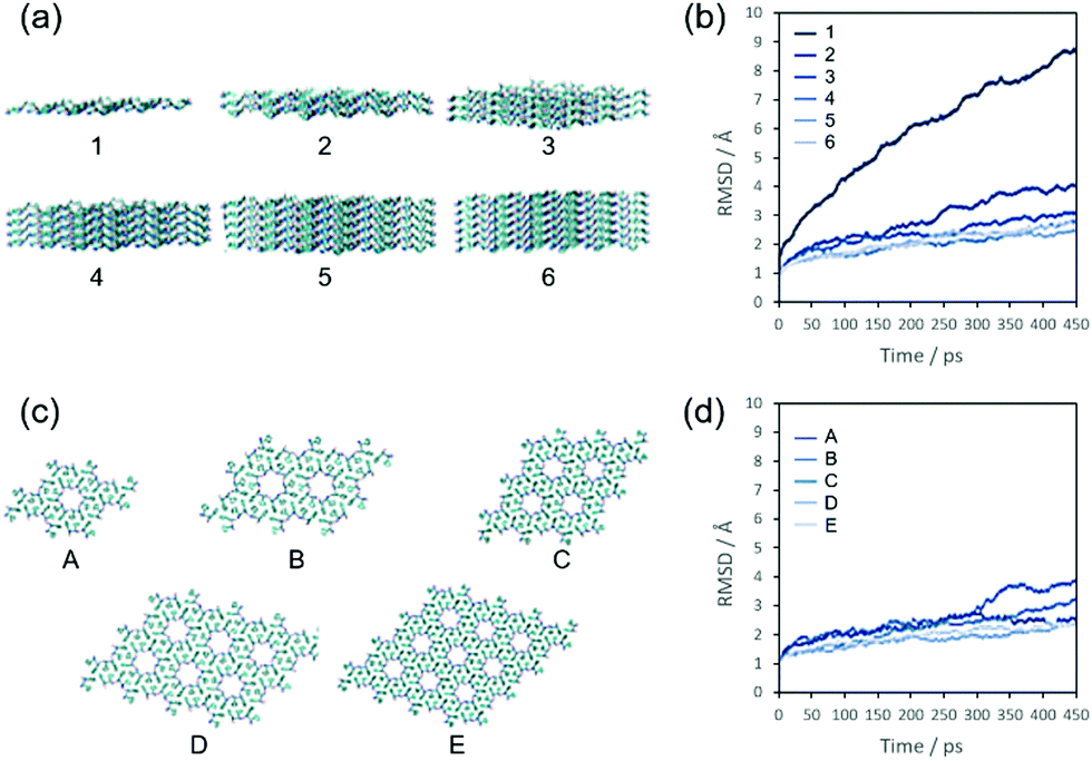Fig. 2 Diphenylalanine structures used in the MD simulations and their RMSDs in solvated atomistic molecular dynamics simulations. (a) Structures with increasing number of FF layers from 1 to 6 (water omitted for clarity). (b) Time dependence of the RMSDs of the structures in (a). (c) Structures with increasing lateral extension from A to E. (d) Time dependence of the RMSDs of the structures in (c).

Next, the lateral extension of an assembly of FF molecules was varied and the number of layers kept constant at 3 (Fig. 2c and d). A visual inspection of the simulations indicated a similar stability for all the examined structures. In accord with this, the RMSDs of the larger structures are essentially identical with the 1 and 2 hexagon structures (A and B, respectively) being slightly more mobile.

The differences in stability in these two sets of simulations is consistent with the high aspect ratio of the fibres: the RMSD dramatically decreases when the small assembly increases in length, which is not the case when the assembly is extended laterally. This means that these structures become much more stable upon elongation as opposed to lateral extension, so the structure will preferentially grow longer instead of wider. This difference in surface energy is a reflection of the different types of intermolecular interactions that stabilise the FF fibres. The layers of molecules in the FF fibres are held together by hydrogen bonding and electrostatic interactions between the termini of the peptides. According to Görbitz,¹³ relatively weaker three-dimensional stacking between aromatic moieties keeps the hexagonal cylinders together (the lateral packing). This results in the molecules preferentially adsorbing onto the ends of a growing structure rather than on its sides, causing the observed high aspect ratio of the fibres.

Temperature stability of FF fibres

FF fibres assemble when they are cooled with the Song method.¹ Therefore, the stability of fibres is clearly a function of temperature. Although there has been previous work on the thermal stability of FF fibres,¹⁷ it has not been done in the solution phase. We therefore decided to investigate the temperature dependence of fibre formation and stability using spectroscopic methods, as they display precise real-time responses to any temperature-induced changes in the fibres and hence allow us to analyse the fibres in situ within their growing environment. This eliminates the need to remove the fibres from solution for analysis, a procedure that has significant practical disadvantages and can change the observed characteristics.³⁶ In particular, we chose to use flow LD because it requires molecules to be aligned in order to detect them, so it only detects fibres: individual molecules, small oligomers and any low aspect ratio assembly/aggregate are invisible. Although there are size limitations with our LD set up due to the annular gap and circumference of the Couette cell, we were able to use it to monitor fibres shorter than ∼1 mm (ESI,† Fig. S2).

At the highest starting temperature of 70 °C, a solution of FF molecules stays as such without assembly for at least 4 hours (ESI,† Fig. S4). Thermal stability measurements were performed by collecting LD spectra while a sample, initially at 70 °C, was cooled in 5 °C steps at a rate of 1 °C min⁻¹ until it reached 20 °C. The sample was then heated back up to 70 °C at the same rate and a spectrum was measured every 5 minutes (i.e. at 5 °C intervals). Data from typical cooling and heating experiments are shown in Fig. 3a and b, respectively, with the spectra offset for clarity (an example of original spectra can be found in Fig. S3 of the ESI,† displayed over a wider wavelength interval). The peaks observed around 265 nm correspond to π–π* transitions in the aromatic part of the molecule and are red-shifted relative to the monomer absorbance (ESI,† Fig. S1) as a result of π-stacking interactions. The phenyl LD signals start to appear when the sample temperature has reached 40 °C (Fig. 3a), indicating that the fibres have become long enough to align in shear flow. The change in baseline as a function of time is due to the increase in light scattering as the fibres become larger, since scattering is a function of wavelength as well as particle size.³⁷ When the solution is heated back up, the dichroic signal decreases, which shows that the fibres do disassemble upon heating with the process being completed by 70 °C (Fig. 3b).

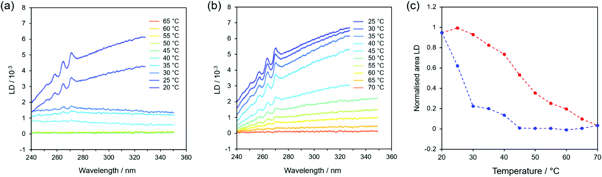Fig. 3 LD signal of fibres forming from 2 mg mL⁻¹ FF monomer solutions as the sample is (a) cooled from 70 °C to 20 °C with a 1 °C min⁻¹ rate and then (b) heated back again to 70 °C at the same rate. LD spectra have been offset for clarity. (c) Plot of the areas under the LD curves of (a) fibres formation (blue, cooling) and (b) fibre dissolution (red, heating) normalised to a maximum value of 1.

In order to appreciate the temperature dependence in a more quantitative way, Fig. 3c shows a plot of the integrated intensity of the 250–270 nm peaks versus temperature (the area under the peaks was evaluated after subtracting the baseline for each spectrum, as shown in ESI† Fig. S5). Fig. 3c shows a clear difference between formation and dissolution for these fibres (the experiment was undertaken slowly enough to ensure that the sample had equilibrated at each temperature). When cooling from 70°C (blue curve in Fig. 3c), no fibres develop until a threshold temperature of about 40 °C is reached, after which they form quickly. This suggests that a nucleation-driven assembly is taking place (see below) with nucleation happening when the system is supersaturated (achieved by heating a sample to 70 °C and then cooling). However, there is no such equivalent for the disassembly process (red curve in Fig. 3c), as dissolution is accompanied by a slower and steady decrease in signal from 20 °C.

The cooling–heating experiment was repeated several times with comparable results (within experimental error), showing that ∼40 °C is indeed the threshold temperature that allows fibres to start assembling when they are cooled from a hot solution. Interestingly, a similar threshold temperature was also found by repeating the experiment at half the cooling rate (and thus double the time), although in this case the integrated LD signal reached it maximum value earlier (35 °C, ESI† Fig. S6). This is a clear indication that kinetic aspects play an important role in the fibre formation.

Kinetics of assembly

Many modelling studies of the kinetics of fibre assembly have been undertaken, most, e.g.ref. 38, including nucleation of a primary fibre – deemed to be the smallest fibre growth unit – followed by fibre growth by monomer addition. Typically experimental data prove more complex than this, requiring secondary nucleation mechanisms such as fibre fragmentation to increase the number of growing ends or the use of one fibre as a template for a second to start growing. Rates of growth as a function of monomer concentration are a key variable in such studies. Unfortunately as noted above, FF fibre formation is crucially concentration dependent, with even a 50% dilution resulting in vesicles and nanotubes forming.¹ We therefore approached our kinetic studies by using multiple repeats of a single concentration with LD to probe lag times for nucleation and kinetics of fibre growth and optical microscopy to give snapshots.

Linear dichroism. If the initial stage of fibre assembly requires a nucleation event, then it should introduce a strong stochastic element into the time dependence of otherwise equivalent (i.e. repeat) experiments. Accordingly, flow LD was used to monitor the kinetics of assembly in a series of experiments where the Couette cell was initially loaded and held at 70 °C for a background spectrum to be taken, the sample was then rapidly cooled to 40 °C, and a spectrum was measured every 5 minutes for 4 hours. Fig. 4a shows typical results from such an experiment. Three stages are apparent: an induction period, lasting about 80 minutes in this case, during which there are no LD-detectable fibres; a second stage during which the phenyl LD peaks appear and then grow rapidly (linearly) in intensity; and a third stage, commencing at about 100 minutes in this case, for which the signal fluctuates about an apparent plateau.

Fig. 4 (a) Normalised integrated intensity of LD spectra versus time during the formation of fibres at 40 °C. (b) Distribution of waiting times before fibre formation was detected. (c) Fraction of experiments (cumulative distribution) in which fibres have been detected within time t (black circles). The blue line is the fit to eqn (1) with λ = 0.03 min⁻¹ and t_g = 8 min.

This experiment was repeated 18 times and the same qualitative pattern was always observed, although the timing of the transitions (particularly between stages 1 and 2) varied as summarised in Fig. 4b. The approximately linear increase in the LD signal observed in stage 2 is consistent with a constant population of fibres (i.e. nucleation of new fibres is much slower than growth), constant orientation parameter S (see ESI†), and the addition of FF to the fibre ends at a constant rate.

The duration of the first stage, and the rapid transition to growth in the second stage, is well explained by nucleation. Nucleation is a stochastic process that has been shown to follow Poisson statistics,³⁹ and so gives rise to an exponential distribution of waiting times for the nucleation event to occur. In the current experiment, however, the nucleation of a single crystal is not coincident with detection. Instead, following a nucleation event, an additional delay, t_g, occurs while the fibres grow long enough to orient sufficiently well under shear to give a detectable LD signal.⁴⁰ Moreover, the nucleation of n fibres might be required before the density of fibres is large enough to be detected. Based on these two considerations it is possible to derive a theoretical cumulative distribution function F(t) (CDF, see ESI†) that can be compared with the fraction of experiments in which fibres have been detected within time t (Fig. 4c). The data show an excellent fit to eqn (1)

F(t) = 1 − e^{−λ(t−t_g)} (1)

corresponding to the case of a single nucleation event occurring at a rate λ and with a growth time t_g prior to detection (see ESI†).⁴¹ The best fit (Fig. 4c) is for physically reasonable parameters, λ = 0.03 min⁻¹, t_g = 8 min. The nucleation rate (on average, one event every 30 minutes) is entirely consistent with Fig. 4b.

However, microscopy images (Fig. 1) clearly show the formation of many fibres during stages 2 and 3 – probably too many to be explained by a nucleation rate of just 0.03 min⁻¹. We therefore conclude that the appearance of multiple fibres during stage 2 must be a consequence of secondary nucleation; this is an autocatalytic nucleation mechanism, and so is consistent with observing many fibres from a small (initial) nucleation rate. Secondary nucleation requires that fibres easily break and the pieces act as nuclei to seed the growth of several fibres. ESI† Fig. S8 shows a fibre which has branched out into many fibres and has a break. This is similar to the secondary nucleation growth of amyloid-β.²⁵

Finally, we observe that the noisy data after 100 min in Fig. 4a (stage 3) is an experimental limitation due to the size of the Couette cell (ESI,† Fig. S2). Once fibres grow to a length that is comparable with the gap between inner and outer walls of the cell, they no longer align with the shear flow—sometimes getting stuck and subsequently breaking. Therefore, only the first two stages of the fibre growth generate useful quantitative LD data. The onset of stage 3 also allows an approximate rate of fibre growth to be determined. In fact, the Couette cell annular gap is 0.25 mm and the fibres take about 28 minutes (t_g + length of stage 2) to get stuck. A fibre of length a bit more than 1 mm fits along the annular gap, so we estimate the fibre growth rate to be about 2 mm h⁻¹ (∼0.6 ± 0.1 μm s⁻¹).

Optical microscopy. The LD technique averages over the whole sample, while the SEM images of Fig. 1 show a range of different fibre sizes but no indication of how they grew to that size. In order to observe the growth of individual fibres, we used a widefield deconvolution optical microscope. The sample was prepared under conditions similar to those used for the spectroscopy experiments (FF solution heated to 70 °C and then rapidly cooled to 40 °C) and was held at 40 °C for the entirety of the optical microscopy measurements. In this experiment, the fibres first appeared at around 5 minutes after the time at which the fibres were cooled to 40 °C. Fig. 5 shows the growth of one fibre over a period of 100 seconds, starting 360 seconds after the beginning of the experiment. It was not possible to measure the full length of the fibres, as they were longer than the field of view of the microscope; however, from a series of images it was possible to measure the speed of growth. It is evident from Fig. 5 that the width of this fibre does not vary much during the experiment (at least once they are long enough to be viewed under the microscope). The length of the fibre in Fig. 5 grows at an initial rate of about 0.6 μm s⁻¹ (in excellent accord with the ∼0.6 μm s⁻¹ from the LD).

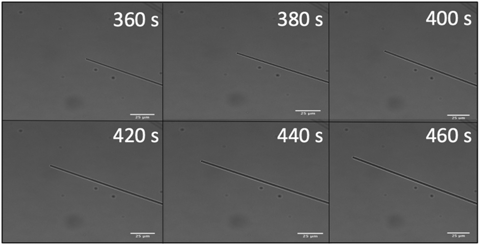Fig. 5 Six frames of a fibre assembling as observed by optical microscopy. The first image was taken 360 seconds after the start of the experiments and the subsequent images were taken at 20 seconds intervals. The scale bar correspond to 25 μm.

Conclusions

The aim of this work was to achieve a better understanding of the growth of FF fibres. A range of complementary experiments and calculations have been performed to that end. SEM images showed that fibres prepared by the method of Song et al.¹ have a hexagonal cross-section, are mostly hollow and display a large range of widths (up to tens of microns) and a high aspect ratio. MD simulations demonstrated that the FF assemblies become much more stable if molecules are added to the ends of a fibre than if they are added to the sides, implying that the fibre growth occurs preferentially along its axis. This is most probably caused by the electrostatic interactions between planes of FF perpendicular to the fibre axis, which are stronger than the lateral stacking interactions between FF molecules within these planes. Therefore, we conclude that thermodynamics plays a large role in determining the large aspect ratio observed in the fibres.

Temperature-dependent LD experiments showed that fibre formation in water did not occur above 40 °C and demonstrated a difference between the formation and the dissolution of the fibres. Kinetic LD studies indicated a slow nucleation followed by a faster growth of fibres with the possibility of secondary nucleation following the fragmentation into smaller initial fibres causing an autocatalytic cascade of growth. It is interesting to note that the nucleation process mentioned by Ishikawa et al.¹² occurs in the dead time of our experiment and presumably relates to a reorganisation of the monomers occurring in the very early stages of what we referred to as the induction period. Their data are therefore not on fibres but on a smaller structure that cannot be flow-oriented. In this work we quantified the Poisson distribution of lag times that occurred and modelled the process to account for the extra delay before detection of fibres by LD. Optical microscopy measurements allowed the direct visualisation of individual growing fibres and showed that the width of a fibre did not change quickly (if at all) during assembly. Microscopy and LD both gave an initial growth rate of fibres to be about 0.6 μm s⁻¹.

Conflicts of interest

There are no conflicts to declare.

Acknowledgements

Financial support from the Engineering and Physical Sciences Research Council (EPSRC, grant EP/F500378/1) for the MOAC Doctoral Training Centre is gratefully acknowledged.

References

1. Y. Song, S. R. Challa, C. J. Medforth, Y. Qiu, R. K. Watt, D. Peña, J. E. Miller, F. V. Swol and J. A. Shelnutt, Chem. Commun., 2004, 1044–1045,  10.1039/B402126F.
2. A. Dehsorkhi, V. Castelletto and I. W. Hamley, J. Pept. Sci., 2014, 20, 453–467.
3. M. M. J. van Rijt, A. Ciaffoni, A. Ianiro, M.-A. Moradi, A. L. Boyle, A. Kros, H. Friedrich, N. A. J. M. Sommerdijk and J. P. Patterson, Chem. Sci., 2019, 10, 9001–9008.
4. I. S. Oliveira, M. Lo, M. J. Araújo and E. F. Marques, Soft Matter, 2019, 15, 3700–3711.
5. E. Kokkoli, A. Mardilovich, A. Wedekind, E. L. Rexeisen, A. Garg and J. A. Craig, Soft Matter, 2006, 2, 1015–1024.
6. A. Trent, R. Marullo, B. Lin, M. Black and M. Tirrell, Soft Matter, 2011, 7, 9572–9582.
7. W. Hwang, D. M. Marini, R. D. Kamm and S. Zhang, J. Chem. Phys., 2003, 118, 389–397.
8. S. M. Acuña, M. C. Veloso and P. G. Toledo, J. Nanomater., 2018, 2018, 8140954.
9. D. Thacker, K. Sanagavarapu, B. Frohm, G. Meisl, T. P. J. Knowles and S. Linse, Proc. Natl. Acad. Sci. U. S. A., 2020, 117, 25272–25283.
10. M. Reches and E. Gazit, Science, 2003, 300, 625–627.
11. M. Reches and E. Gazit, Nano Lett., 2004, 4, 581–585.
12. M. S. Ishikawa, C. Busch, M. Motzkus, H. Martinho and T. Buckup, Phys. Chem. Chem. Phys., 2017, 19, 31647–31654.
13. C. H. Görbitz, Chem. – Eur. J., 2001, 7, 5153–5159.
14. C. H. Görbitz, Chem. Commun., 2006, 2332–2334.
15. L. Niu, X. Chen, S. Allen and S. J. B. Tendler, Langmuir, 2007, 23, 7443–7446.
16. I. D. Thompson and L. L. Hench, Proc. Inst. Mech. Eng., Part H, 1998, 212, 127–136.
17. L. Adler-Abramovich, M. Reches, V. L. Sedman, S. Allen, S. J. B. Tendler and E. Gazit, Langmuir, 2006, 22, 1313–1320.
18. M. Yemini, M. Reches, E. Gazit and J. Rishpon, Anal. Chem., 2005, 77, 5155–5159.
19. A. Krylov, S. Krylova, S. Kopyl, A. Krylov, F. Salehli, P. Zelenovskiy, A. Vtyurin and A. Kholkin, Crystals, 2020, 10, 224.
20. J. Jeon, C. E. Mills and M. S. Shell, J. Phys. Chem. B, 2013, 117, 3935–3943.
21. P. Tamamis, L. Adler-Abramovich, M. Reches, K. Marshall, P. Sikorski, L. Serpell, E. Gazit and G. Archontis, Biophys. J., 2009, 96, 5020–5029.
22. A. Manandhar, M. Kang, K. Chakraborty, P. K. Tang and S. M. Loverde, Org. Biomol. Chem., 2017, 15, 7993–8005.
23. C. Guo, Y. Luo, R. Zhou and G. Wei, ACS Nano, 2012, 6, 3907–3918.
24. W.-F. Xue, S. W. Homans and S. E. Radford, Proc. Natl. Acad. Sci. U. S. A., 2008, 105, 8926–8931.
25. S. I. A. Cohen, S. Linse, L. M. Luheshi, E. Hellstrand, D. A. White, L. Rajah, D. E. Otzen, M. Vendruscolo, C. M. Dobson and T. P. J. Knowles, Proc. Natl. Acad. Sci. U. S. A., 2013, 110, 9758–9763.
26. B. Nordén, A. Rodger and T. R. Dafforn, Linear dichroism and circular dichroism: a textbook on polarized spectroscopy, Royal Society of Chemistry, Cambridge, 2010.
27. R. Marrington, T. R. Dafforn, D. J. Halsall, M. Hicks and A. Rodger, Analyst, 2005, 130, 1608–1616.
28. M. R. Hicks, A. Rodger, Y. Lin, N. C. Jones, S. V. Hoffmann and T. R. Dafforn, Anal. Chem., 2012, 84, 6561–6566.
29. T. R. Dafforn and A. Rodger, Curr. Opin. Struct. Biol., 2004, 14, 541–546.
30. F. H. Allen, Acta Crystallogr., Sect. B: Struct. Sci., 2002, 58, 380–388.
31. B. R. Brooks, C. L. Brooks III, A. D. Mackerell Jr., L. Nilsson, R. J. Petrella, B. Roux, Y. Won, G. Archontis, C. Bartels, S. Boresch, A. Caflisch, L. Caves, Q. Cui, A. R. Dinner, M. Feig, S. Fischer, J. Gao, M. Hodoscek, W. Im, K. Kuczera, T. Lazaridis, J. Ma, V. Ovchinnikov, E. Paci, R. W. Pastor, C. B. Post, J. Z. Pu, M. Schaefer, B. Tidor, R. M. Venable, H. L. Woodcock, X. Wu, W. Yang, D. M. York and M. Karplus, J. Comput. Chem., 2009, 30, 1545–1614.
32. J. C. Phillips, R. Braun, W. Wang, J. Gumbart, E. Tajkhorshid, E. Villa, C. Chipot, R. D. Skeel, L. Kalé and K. Schulten, J. Comput. Chem., 2005, 26, 1781–1802.
33. E. F. Pettersen, T. D. Goddard, C. C. Huang, G. S. Couch, D. M. Greenblatt, E. C. Meng and T. E. Ferrin, J. Comput. Chem., 2004, 25, 1605–1612.
34. R. Marrington, T. R. Dafforn, D. J. Halsall and A. Rodger, Biophys. J., 2004, 87, 2002–2012.
35. R. Marrington, M. Seymour and A. Rodger, Chirality, 2006, 18, 680–690.
36. L. L. E. Mears, E. R. Draper, A. M. Castilla, H. Su, Zhuola, B. Dietrich, M. C. Nolan, G. N. Smith, J. Doutch, S. Rogers, R. Akhtar, H. Cui and D. J. Adams, Biomacromolecules, 2017, 18, 3531–3540.
37. G. Dorrington, N. P. Chmel, S. R. Norton, A. M. Wemyss, K. Lloyd, D. Praveen Amarasinghe and A. J. B. R. Rodger, Biophys. Rev., 2018, 10, 1385–1399.
38. K. Eden, R. Morris, J. Gillam, C. E. MacPhee and R. J. Allen, Biophys. J., 2015, 108, 632–643.
39. T. W. Barlow and A. D. J. Haymet, Rev. Sci. Instrum., 1995, 66, 2996–3007.
40. J. McLachlan, D. J. Smith, N. P. Chmel and A. Rodger, Soft Matter, 2013, 9, 4977–4984.
41. S. Jiang and J. H. ter Horst, Cryst. Growth Des., 2011, 11, 256–261.

---

Footnote

† Electronic supplementary information (ESI) available. See DOI: 10.1039/d0cp05477a

---