
 Open Access Article
 This Open Access Article is licensed under a
 Creative Commons Attribution 3.0 Unported Licence
Temperature evolution in IR action spectroscopy experiments with sodium doped water clusters†
Daniel
Becker
a,
Christoph W.
Dierking‡
a,
Jiří
Suchan
b,
Florian
Zurheide
a,
Jozef
Lengyel
 c,
Michal
Fárník
d,
Petr
Slavíček
b,
Udo
Buck
e and
Thomas
Zeuch
*a
c,
Michal
Fárník
d,
Petr
Slavíček
b,
Udo
Buck
e and
Thomas
Zeuch
*a
aUniversität Göttingen, Institut für Physikalische Chemie, Tammannstr. 6, 37077 Göttingen, Germany. E-mail: tzeuch1@gwdg.de
bDepartment of Physical Chemistry, University of Chemistry and Technology, Technická 5, 16628 Prague 6, Czech Republic
cLehrstuhl für Physikalische Chemie, Technische Universität München, Lichtenbergstr. 4, 85748, Garching, Germany
dJ. Heyrovský Institute of Physical Chemistry, v.v.i., Czech Academy of Sciences, Dolejškova 3, 182 23 Prague 8, Czech Republic
eMax-Planck Institut für Dynamik und Selbstorganisation, Am Faßberg 17, D-37077 Göttingen, Germany
First published on 16th December 2020
Abstract
The combination of supersonic expansions with IR action spectroscopy techniques is the basis of many successful approaches to study cluster structure and dynamics. The effects of temperature and temperature evolution are important with regard to both the cluster synthesis and the cluster dynamics upon IR excitation. In the past the combination of the sodium doping technique with IR excitation enhanced near threshold photoionization has been successfully applied to study neutral, especially water clusters. In this work we follow an overall examination approach for inspecting the interplay of cluster temperature and cluster structure in the initial cooling process and in the IR excitation induced heating of the clusters. In molecular simulations, we study the temperature dependent photoionization spectra of the sodium doped clusters and the evaporative cooling process by water molecule ejection at the cluster surface. We present a comprehensive analysis that provides constraints for the temperature evolution from the nozzle to cluster detection in the mass spectrometer. We attribute the IR action effect to the strong temperature dependence of sodium solvation in the IR excited clusters and we discuss the effects of geometry changes during the IR multi-photon absorption process with regard to application prospects of the method.
1 Introduction
Size-resolved studies of the structure and dynamics of hydrogen bonded clusters shed light on the molecular level interactions of condensed matter and the gradual evolution of macroscopic properties with cluster size.1–14 With increasing computational and predictive power the theoretical description becomes more precise even for larger systems bridging the gap between macroscopic and cluster size specific properties. A recent example is the comprehensive analysis of the emergence of the structural motif of ice I in the smallest possible water clusters by molecular beam experiments and molecular simulations.15 This study places this lower limit to water clusters with around 90 water molecules and draws the conclusion that the phase equilibrium between the liquid and crystalline solid state appears in this size range through heterophasic oscillations in time, a process without analog for macroscopic water. The preparation of the clusters in this dynamic state is highly sensitive to cluster temperature and cooling rates during cluster synthesis in the supersonic expansion. Different to trapping techniques with ions,16,17 recently extended to nanoparticles,18 temperature control is still very challenging for experiments with neutral clusters. However, huge efforts have been made to assess temperatures (and more recently cooling rates) in supersonic expansion experiments applying complementary experimental approaches19–21 and detailed numerical simulations of the gas and clustering dynamics.22 The final cluster temperatures derived in these studies have been used as a support to interpret many temperature sensitive, size resolved experiments,15,19–21,23 but so far a detailed description of the method has not been presented. Therefore, in the first part of this work we gather this information and provide constraints for temperature assessments as a function of expansion conditions.For water clusters, the upper cluster temperature is limited in supersonic expansions due to the evaporative cooling process,24 while black body radiation at 300 K causes fragmentation in temperature controlled ion trap experiments.16,25 In the present study we apply an action effect which is connected to changes in Na solvation in water and other hydrogen bonded clusters.26–28 It turned out that IR excitation and near threshold photoionization of such singly Na doped clusters has several beneficial properties. First, the photoionization is fragmentation free under these conditions.29 Second, the positive IR enhanced signal is obtained simultaneously for each cluster size of the distribution and third, the IR excitation can be fragmentation free at least for certain stable cluster configurations.30,31 Molecular simulations have shown that heating increases the abundance of Na atoms in configurations with low ionization energy explaining the positive IR signal.27,32 However, at elevated temperatures evaporative cooling may play an important role. To analyse these competitive processes we have examined the dependence of the ion signal as a function of the delay time between the IR and ionizing UV laser pulse and we simulated the solvation of the Na atom in (H2O)7 clusters and the evaporative cooling process over a broad range of cluster temperatures. Combining these examinations we arrive at constraints for the temperature evolution in this type of experiment from cluster synthesis to cluster detection. We describe the general procedure and give several examples of its application in Section 2. In Sections 3 and 4 we expand the explored temperature range well beyond 180 K as we try to disentangle the effects of sodium solvation and evaporative cooling on the ion signal after heating by an IR laser pulse. Finally, we shortly discuss future application of this technique for water and other sodium doped, hydrogen bonded clusters in Section 5.
2 Experiment and molecular beam properties
2.1 Cluster experiments
In this section, we will inspect the gas and clustering dynamics of supersonic expansions through conical nozzles of gaseous water vapor diluted by a carrier gas and in the version of a pure expansion. But first we give a short outline of the conduction of the cluster experiments. We have chosen to use conical nozzles of much smaller diameter compared to those used in the Laval nozzle experiments for studying water aggregation and nucleation in continuous supersonic expansions.33,34 In the present case, the clusters are typically not produced under equilibrium conditions. Their temperatures were previously evaluated from the measured velocities using the energy balance of the beam and the simulated relaxation process of the clusters by the carrier gas.19,20 The disadvantage of the complicated cluster temperature evaluation is compensated by the high accuracy of the measurement of the cluster size distributions, either by scattering from a He beam for smaller sizes35 or by the Na doping technique for the larger ones.29,36–38The experiments in this work are carried out in conventional molecular beam machines. Schemes thereof are shown in recent articles.15,21,28,38 The cluster size for pure water expansions is essentially determined by the density n0 and the temperature T0. The quantitative relation is published in ref. 37. We add the carrier gases He, Ne and Ar to the expansion in order to vary the cluster temperature by collisional cooling. The parameters that determine this process are shown in the explanation of eqn (3) below.
The crucial ingredient of the experiments is the method of size selection for the neutral water clusters. In the case of the earlier scattering experiments with a He beam in the Buck group the cluster sizes are separated and detected by the different deflection angles in an experiment with high angular resolution. Here, the IR spectroscopy is carried out in the usual way by vibrational predissociation and the depletion of the signal.
The larger clusters are doped with Na atoms which are produced in a pick-up cell. Because of the low ionization energy of Na which is further lowered to around 3 eV by the interaction with water,29 the system is easily photoionized by one photon using commercially available lasers. This arrangement has two advantages. The low ionization energy prevents any interferences with the direct ionization of water which takes place at much higher energies around 10 to 12 eV. In addition, the potential curves of the ionic and neutral configurations are quite similar so that the ionization directly at the threshold can avoid the usual fragmentation, since both the photon and the cationic cluster do not carry any significant excess energy. In this work the photoionization is performed at 385 nm (3.2 eV). The IR spectroscopy is carried out by the addition of the UV- to the IR-signal so that the signal enhancement is measured. The detailed mechanism is reinspected and discussed in Sections 3 and 4. Detailed descriptions of the method are found in ref. 15 and 32, more details on the experiments of this work are given in the ESI.†
2.2 Cluster temperature
A method that allows the assessment of the cluster temperature developed in the Buck group is the energy balance of the cluster beam which will be treated in detail here. On the one hand the predictions of the approach are validated by several unambiguous experiments on cluster melting and isomerism accompanied by high level molecular simulations. On the other hand we have a range of conditions where we have higher uncertainties. Therefore we cannot provide a general assessment of uncertainties covering the full range of expansion conditions (pure water expansions, expansions with carrier gases He, Ne, Ar at low and very high fractions). However, at the and of this section we try to give uncertainty margins based on the detailed discussion of the method below. For readers more interested in the new, temperature sensitive simulations and experiments (Sections 3–5) we start this section with a short summary. For weak expansions with stagnation pressures around 1 bar and a significant fraction of water (0.2 or more) final temperatures of 150 K or more are reached. Higher stagnation pressures and lower water fractions (0.2 or less) result in low cluster temperatures of around 70 K or less. The intermediate temperature range can be interpolated between the two boundaries, but there are differences with regard to the applied carrier gases. This rough assessment is bolstered by size resolved IR spectroscopic studies.15,19–21,28 We think this empirical evidence is sufficient to interpret the new experiments and simulations of this work. However, there are two other methods which have been used to assess the cluster temperature. They allow for the more consistent presentation of the energy balance model in this section including uncertainty estimates.An interesting approach to determine the cluster temperature is the deexcitation of the cluster by high resolution inelastic He atom scattering. Buck and co-workers have used this experimental method to measure the intermolecular modes of the surface of the clusters which correspond to the surface phonons of the solid.39,40 For pure water expansions and mean cluster sizes between ![[n with combining macron]](https://www.rsc.org/images/entities/i_char_006e_0304.gif) = 80 and = 194 temperatures between 130 K and 100 K were obtained.
= 80 and = 194 temperatures between 130 K and 100 K were obtained.
Moreover, the availability of the important experimental quantity of the size distribution enabled the validation of gas dynamics approaches to the cluster growth process at a molecular level.41,42 The kinetic, first-principle approach to the condensation phenomenon based on a microscopic view of the interaction rates has to be coupled to the properties of the rapidly changing flow. The direct simulation Monte Carlo (DSMC) method was used to tackle this problem for relatively low density plumes.41 As the method has high computational cost at high plume densities, the group of Gimelshein has developed a more robust approach that combines the Eulerian continuum approach for gas flow with a DSMC-like particle based algorithm for nucleation and cluster evolution.42
The energy balance of a typical adiabatic expansion is given by the enthalpy of the gas at the starting temperature H0(T0) and after the expansion by the enthalpy of the final temperature H(T) and the remaining kinetic energy Ekin. In case of cluster formation we have to add two components, the condensation energy Econ which increases the available energy during the starting period and the enthalpy of the cluster Hc(Tc), which contains the cluster temperature Tc and which appears as final contribution when the expansion is completed.
| H0(T0) + Econ = H(T) + Ekin + Hc(Tc). | (1) |
| (A) + (B) = (C) + (D) + (E). | (2) |
It is obvious from this equation that, if the kinetic energy is measured, we can easily get information on the cluster temperature in a qualitative way. Low cluster temperatures will lead to high kinetic energies and vice versa. Let us at first discuss the different contributions separately.
(A) The enthalpy is given in Kelvin (K) by H0 = CpT0 = (f + 2)/2·T0. Cp is the heat capacity at constant pressure (reference reservoir). It can be expressed by the number of degrees of freedom f with f = 3 for atoms and f = 6 for molecules with three rotations.
(B) The condensation energy is given by Econ = xcncEbin. The energy released by the cluster formation process is the binding energy which is well known and which can be assumed to be about Ebin = 4532 K per unit for clusters larger than nc ≥ 14.22xc is the fraction of clusters and nc is the cluster size. The number of water clusters which contribute to this energy is not easy to get. It is especially for larger cluster smaller than the cluster size nc. Smaller clusters are usually formed by the addition of molecules, while the larger ones show the tendency of coagulation of smaller clusters. Thus this effective number is usually smaller than the nominal cluster size. One should note that for expansions producing large clusters (high average nc) the cluster fraction xc can be well below 1% although the water monomer mass is still below 50%.
(C) The enthalpy after the expansion H is usually quite small in our expansions so that it can be left out in the energy balance.
(D) The kinetic energy term Ekin is an important contribution. It is given in K by Ekin = 60.2v2![[m with combining macron]](https://www.rsc.org/images/entities/i_char_006d_0304.gif) . Here the velocity v is measured in multiples of 1000 m s−1 and the averaged mass in atomic units. Then the energy results in K. The average mass is given by = xama + xcncmm + (1 − xc)mm with the fraction xa of the atomic carrier gas and the fraction of the clusters xc. The atomic mass of the carrier gas is ma and that of the cluster monomer is mm.
. Here the velocity v is measured in multiples of 1000 m s−1 and the averaged mass in atomic units. Then the energy results in K. The average mass is given by = xama + xcncmm + (1 − xc)mm with the fraction xa of the atomic carrier gas and the fraction of the clusters xc. The atomic mass of the carrier gas is ma and that of the cluster monomer is mm.
(E) The final term is the energy of the clusters Hc = xcCcTc with the cluster heat capacity Cc and the cluster temperature Tc (two degrees of freedom belonging to molecular interactions have been transferred to directed motion in the beam). The cluster heat capacities at constant volume are taken from ref. 41. They are per unit Cc = 8.1 for clusters larger than nc ≥ 14.
The cluster relaxes from the newly available temperature T0′, which consists of the enthalpy and the condensation energy, to the cluster temperature Tc by collisions with the carrier gas according to
 | (3) |
 . Here μij is the reduced mass, and the two indices i and j mark the carrier gas and the constituent cluster. The factor (8/π)1/2 = 1.596, which also appears in the formula when the relative energy is calculated, is contained in the prefactor 3.87.
This general formulation in reduced notation allows us to solve the differential equation for a series of parameters. The results are plotted in Fig. 1. For each B the resulting Tred is available. The points in the figure mark the results for water-9, for water-6 expanded in carrier gases and larger pure water clusters in unseeded expansions.
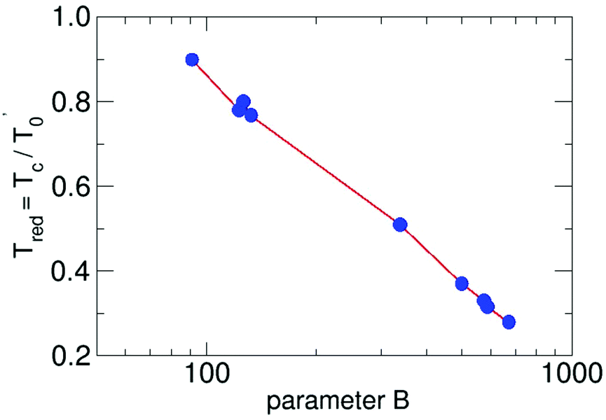 | ||
| Fig. 1 The reduced cluster temperature as a function of the the reduced parameter B. The red lines connect the calculated points of the results of the solution of eqn (3) in a logarithmic scale. | ||
They will be discussed in the following pages. By using this plot we have to reduce the B value, since the value for the density or the pressure in the formula is that of the source. But what counts is the local density. Large B (and thus large densities of the carrier gas) lead to small Tred (and thus small cluster temperatures Tc), a result which should be expected. The definition of the used parameters are presented in Table 1. We note that the reduced cluster temperature shows a logarithmic trend and it would be interesting to see if it is connected to an invariant property like the condensation energy. To this end, cluster temperatures in supersonic expansions should be assessed with the presented energy balance model for other substances. For the methanol hexamer a comprehensive analysis, similar to the water hexamer (Table 3) case discussed below, is available,26 which is a good starting point for a more detailed analysis of cluster temperatures in seeded and unseeded methanol expansions.
| Parameters | Definitions |
|---|---|
| E con | Condensation energy |
| n c | Cluster size |
| x c | Fraction of clusters (molecular/mass fractions are much higher) |
| E bin | Binding energy within the cluster |
| x a | Fraction of atomic carrier gas |
| m a | Atomic mass of the carrier gas |
| m m | Mass of the cluster monomers |
| T c | Cluster temperature |
| C c | Cluster heat capacity |
| T 0′ | Temperature from enthalpy and condensation energy |
| T red | T c/T0′ |
2.3 Examples
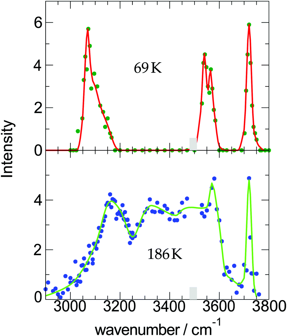 | ||
| Fig. 2 Measured OH-stretch spectra of water-9 for two different cluster temperatures; the intensity corresponds to the strength of the action effect, here the depletion of the ion signal. The data are taken from ref. 19. | ||
The experimental conditions are listed in Table 2. We see that the main difference in the two experiments is the much higher He pressure in the first one. This should lead to a smaller cluster temperature which is reflected in the higher kinetic energy. Now let us try to calculate this temperature. From the experiment we know that the fraction of water molecules, which end up in the clusters is 0.77 and the average cluster size is c = 6.5. We calculate the enthalpy H0 = 976 K and 960 K, the kinetic energy Ekin = 3141 K and 2853 K, and the cluster enthalpy Hc = 5.158 Tc and 6.206 Tc for the two experiments. The cluster temperature can be replaced by Tc = TredT0′ in which Tred is the solution of eqn (3) and T0′ the new temperature. Based on the parameters B = 586 and B = 132 we get for Tred 0.29 and 0.78.
| Properties | Set(1) | Set(2) |
|---|---|---|
| Total pressure/bar | 2.3 | 1.0 |
| Fraction of water | 0.167 | 0.20 |
| He pressure/bar | 1.9 | 0.8 |
| Nozzle temperature/K | 355 | 343 |
| Velocity/(m s−1) | 1654 | 1466 |
| Cluster temperature/K | 69 | 186 |
Therefore we calculate for the energy balance of the two arrangements
| (1) 976 + Econ = 3141 + 5.158TredT0′ = 3141 + 1.496T0′ |
| (2) 960 + Econ = 2853 + 6.206TredT0′ = 2853 + 4.841T0′. |
For Econ we make some additional reasonable assumptions Econ = xcncEbin. Based on xc = 0.167 × 0.77 for (1) and xc = 0.200 × 0.77 for (2), and nc = 6.1 and Ebin = 3323 K for both of them, we get for (1) 2592 K and for (2) 3122 K. The difference is caused by the different values for the amount of water in the expansion. Now the subtraction (1) and (2) gives the value for T0′ = 239 K. This leads to the two cluster temperatures of (1) 69 K and (2) 186 K which are also listed in Table 1. The procedure of the determination of the cluster temperature is pretty complicated. For this case, however, the data are of high quality so that the error is estimated to be 69 K ± 10 K and 186 K ± 20 K.
A similar experiment has been carried out for water hexamers at two closely related temperatures to get information about the structure. Hexamers are the first water clusters with a 3-dimensional structure.44 They appear in four closely related isomeric structures. The rotational spectra measured by the groups of Saykally45 and Pate46 showed a clear evidence for the cage structure, while our measurement of the OH-stretch spectrum was interpreted as coming from the book isomer.20 This turned out to be due to an error in the calculation. A very detailed and sophisticated calculation by the group of Skinner, however, came to the conclusion that also our measurement at 40 K is in full agreement with the prediction based on the cage isomer.21,47 The measured spectrum at 60 K is well reproduced by the cage isomer and a small admixture of the book isomer as is predicted by theory.
For the experiment with water hexamers the results are listed in Table 3. In this case the cluster temperatures are low and not very different from each other. Thus the energy balance gives
| (1) 976 + 2594 = 3134 + 5.158TredT0′ = 3134 + 1.908T0′ |
| (2) 824 + 547 = 1198 + 1.088TredT0′ = 1198 + 0.272T0′. |
| Properties | Set(1) | Set(2) |
|---|---|---|
| Total pressure/bar | 2.3 | 2.3 |
| He pressure/bar | 1.9 | 2.2 |
| Fraction of water | 0.167 | 0.035 |
| Nozzle temperature/K | 355 | 323 |
| Velocity/(m s−1) | 1657 | 1667 |
| Cluster temperature/K | 60 | 40 |
The B-values for the calculation of the cluster cooling are slightly smaller for experiment (1), because of the smaller He pressure and the larger temperature. Therefore we have the result for experiment (1) B = 502 and Tred = 0.37 and for experiment (2) B = 731 and Tred = 0.25. Now the subtraction (1) and (2) gives T0′ = 161 K. These results lead to the corresponding cluster temperatures Tc = 60 K for (1) and Tc = 40 K for (2).
| Gas | p/bar | Gas | p/bar | T 0 >/K | T c/K |
c
|
|---|---|---|---|---|---|---|
| Ne | 2.30 | H2O | 1.00 | 385 | 100.5 | 77 |
| Ne | 1.30 | H2O | 1.00 | 385 | 100 | 59 |
| Ne | 1.30 | H2O | 1.00 | 433 | 100 | 39 |
The temperatures of the clusters are in spite of the partly different conditions surprisingly similar. The increase of the temperature T0 from 385 K to 433 K has no influence on Tc but decreases the average cluster size . The increase of the Ne pressure from 1.3 to 2.3 bar with constant H2O pressure and constant temperature T0 leads to an increase of the cluster size. The expected lower cluster temperature is compensated by the slight increase of the temperature caused by the increased condensation energy due to the formation of larger clusters.
The detailed molecular simulation of the beam properties is validated by the agreement of the predicted size distributions with the experiment.24 This allows us to take the first example in the table, 2.3 bar Ne and 1.0 bar water pressure at 385 K and a predicted cluster temperature of 100 K, as a reference to verify the usability of eqn (1) to calculate cluster temperatures:
(A) The enthalpy is given by H0 = (0.7 × 2.5 + 0.3 × 4.0) × 385 = 1136 K.
(D) The kinetic energy is given by Ekin = 60.2 × 1.0932 × = 1573 K with = 0.7 × 20 + 0.3 × 18 × (0.006 × 77 + 0.994). The measured velocity is 1093 m s−1, the average cluster size is = 77 and the cluster fraction is 0.006.
(E) The enthalpy of the cluster is given by Hc = 0.3 × 0.006 × 77 × 8.1 × 100 = 112 K.
(B) To get information on the condensation energy is probably the most difficult part. It is given by Econ = 0.3 × 0.006 × 77 × Ebin = 628 K. Here we used the simple model that all the clusters are produced by single molecule addition and their binding energy is available. For the cluster size we take = 77. The complete energy balance, however, gives based on the known value of Tc = 100 K, a value which is about 90% of the assumed temperature for = 77. This means that the cluster formation for larger clusters is dominated by coagulation so that the number of clusters involved in the determination of the condensation energy goes down.
To summarize, we have to know in addition to the measured cluster velocity the average cluster size, the cluster fraction and the condensation energy. While the first three quantities can be measured, especially the last information is not easy to get. Therefore it is advisable to use configurations in which the contributions of this term are quite similar so that by using differences of the interacting energies this problem is bypassed.
We would like to discuss some results of the cluster temperature which have been obtained in other important experiments with water clusters in the light of the accurate results so far presented in the Ne expansions. The results are shown in Table 5. In a ground-breaking experiment the onset of the crystallization of size-selected water clusters was measured.28 Later on we discovered that the transition size depended on the cooling rates, which are closely correlated with the final cluster temperature.21 The transition occurs for larger clusters at lower final temperatures and thus higher cooling rates in the region of the freezing temperature.15
The experimental conditions of the experiments on water crystallization which we have carried out are presented in Table 5. The experiment with Ne as carrier gas is exactly that for which the cluster temperature has been calculated.22 The two experiments with He as carrier gas differ only slightly in the pressure of the carrier gas so that the cluster temperatures are quite similar. The other experimental conditions have only minor influence on the results. The two examples of the Ar expansions are carried out at about the same conditions except for the carrier gas pressure which is in one case much lower and leads to a much higher cluster temperature. Thus the energy balances give
| (1) 1012 + 1218 = 1752 + 3.11Tc |
| (2) 945 + 1122 = 1949 + 2.86Tc |
These data turned out to be quite important to find the lowest cluster size of about 90 water molecules for the transition to the ice configuration. Only the weak argon expansion at 1 bar provided the critical conditions: a high cluster temperature and therefore a low cooling rate below 200 K and a sufficiently large average cluster size.15 The bulk of experimental conditions discussed in this paper with final temperatures of 100 K and below (and thus higher cooling rates at the freezing temperature around 180 K48) produces vitrified amorphous clusters at n = 100, 200 and above: the lower the final cluster temperature, the higher the critical cooling rate at 180 K, and the higher the critical onset size.15,21,48 This illustrates that the IR analysis of critical cluster size for the onset of crystallization is consistent with temperature predictions of the energy balance model.
For pure water clusters we have an interesting data set available for which at the same temperature T0 and different water pressures the beam velocities after the expansion have been measured. These values are used to calculate the cluster temperatures. This is a practical realization of the formula presented in eqn (1). The sizes are based on the well known empirically determined formulas.49 The data are shown in Table 6.
| No. | T 0/K | p/bar | Size c |
v/ms−1 | T c/K |
|---|---|---|---|---|---|
| 1 | 428 | 1.2 | 47 | 1316 | 177a |
| 2 | 428 | 1.7 | 85 | 1355 | 135b |
| 3 | 428 | 2.2 | 139 | 1384 | 116 |
| 4 | 428 | 2.6 | 181 | 1394 | 106 |
| 5 | 428 | 3.2 | 258 | 1415 | 103 |
| 6 | 428 | 4.0 | 398 | 1442 | 96 |
| 7 | 428 | 4.8 | 526 | 1461 | 93 |
As already mentioned, we have to know, in addition, the cluster fraction and the amount of the condensation energy. The cluster fraction is estimated from the result of the calculation given in Table 7 which gives 0.010 for the size range treated here. The amount of condensation energy is more difficult to determine. By comparison of a series of calculated and measured examples we arrived at a correction factor of about 0.7, by which we multiply the cluster size in order to account for the possible cluster coagulation in the forming process. For small clusters slightly higher values of 0.8 and 0.75 are used. These values are marked in Table 6 by Tac and Tbc. The results demonstrate that with increasing pressure the cluster size goes up and the cluster temperature goes down. The reason is in both cases the increasing pressure of the carrier gas increasing the amount of free water molecules (less heat release) and the beam velocity (more kinetic energy).
As for the experimental determination of the cluster temperature, we have developed a completely different method compared to the situation with carrier gases. To measure the low energy surface vibrations of clusters, we have introduced the method of He atom scattering. The inelastic energy transfer is detected by time-of-flight analysis of the scattered He atoms. In the case of argon clusters, collective breathing vibration of the solid icosahedral sphere have been detected.50 For water clusters the O·O·O bending motion between adjacent hydrogen bonds on the amorphous cluster surface were measured.51 In this context we found out that special regions of the time-of-flight spectra can be attributed to the deexcitation of the cluster at finite temperature. Based on the assumption that the initial vibrational state can be described by the temperature Tc the cross section for vibrational deexcitation of the clusters gives the corresponding information.39,40 The results for the cluster temperatures based on the deexcitation experiments are presented in Table 7. For experiment 1 we used directly the data of ref. 40 because of their higher reliability.
Concerning the cluster temperatures we have again direct calculations to fit experimental results for several quite different expansion conditions.42 In one case also the temperature was calculated by the Gimelshein group. This example is added in Table 7.
We find an interesting agreement for the cluster temperature of the results of the Table 6 based on the energy balance and the experimental and theoretical results of Table 7. We have to compare the data sets 2, 4, and 6 of Table 6 with the set 1, 2, and 3 of Table 7. We observe good agreement for nc = 85 and 135 K with nc = 80 and 130 K, for nc = 181 and 106 K with nc = 194 and 101 K, and finally those for nc = 398 and 96 K with nc = 365 and 90 K. The size range is quite similar, although the source conditions are quite different. Since the results of Table 7 are either based on reliable calculations or authoritative experiments, we conclude that the assumptions for the condensation energy we have used for the calculations of the cluster temperature of Table 6 are quite realistic.
In this section a broad range of experiments and simulations with very different expansions conditions are discussed, and we think that for several cases quite consistent temperature estimates have been provided. We try to summarize the key results of this analysis by discussing three temperature ranges.
Range A (“warm”): first we can state around 1 bar we always get temperatures in the 150 to 180 K window and the carrier gas effect on temperature is even for Ar less pronounced (see Table 5). Furthermore, evaporative cooling limits the achievable temperatures. Above 150 K we estimate the accuracy to be around ±15 K.
Range B (“medium”): this is the range of temperatures from about 70 to 130 K. These temperatures can be reached under very different expansion conditions. At stagnation pressures around 3 bar temperatures approach 100 K in pure expansions. Adding carrier gases the temperature goes down, more strongly for Ar compared to He. This Argon effect can be seen e.g. in experiments of Suhm and Wassermann52 which lead to controlled Argon coating of ethanol clusters at elevated Argon fractions in the expansion. Neon is a special case, its mass is similar to that of water, allowing for the detailed simulations of the clustering dynamics in our experiment by Gimelshein24 (see Table 4). Neon clearly has a lower effect on the final cluster temperatures compared to He and Ar; it is similar to pure expansions (Table 6). For the pure expansions the energy constraints are high in our experiments, the kinetic energy (beam velocity) and even condensation energies (size distribution) are reasonably well characterized. Here, we estimate the accuracy to be ±15 K. For the seeded expansions it is lower, may be ±25 K.
Range C (“cold”): for reaching temperatures in the 50 K range, high fractions of carrier gases have to be used, then especially for Argon stagnation pressures around 2 bar can be sufficient (Table 5). Similar to the upper range of temperatures we have a limitation at about 30 K by the translational temperature of the carrier gas.24 In this low temperature range we estimate the accuracy to be ±15 K, it may be higher for selected cases where it is coupled to spectroscopic evidence (see Table 3).
3 Simulated temperature effect on sodium solvation
The temperature evolution of sodium-doped water and other hydrogen-bonded clusters can be also examined by the temperature evolution of the ionization probability using ab initio calculations. In our previous studies, we have focused on the size dependence of structural motifs. In the region of the appearance ionization energy Na+⋯e pairs are formed, while surface attached neutral sodium atoms dominate the high ionization energy region.32,53 In our previous study, we performed a detailed analysis of the change of structural preference with increasing temperature for small Na(H2O)n clusters, with n = 2, 3.32 These clusters are small enough so that the whole energy landscape can be mapped and calculated with high-level ab initio methods. The resulting energies can then be weighted by Boltzmann factors. We could observe from this analysis that the onset of ionization should indeed shift to lower energies with increasing temperature for these small clusters. These findings were further supported by molecular dynamics simulations for small clusters. Similar observations were also made for an analogical system of sodium deposited on methanol clusters.27Even for the small clusters, however, the question of convergence was problematic due to a relatively short duration of the ab initio simulations. Furthermore, complexes of sodium with small clusters are not necessarily representative for larger clusters. The onset of ionization only shifts weakly in clusters with more than 4 water units.32,54 Here, we have attempted to provide converged results with a reliable electronic structure method, choosing a cluster with 7 water molecules. The following issues have to be considered. First, the energy landscape for larger clusters gets progressively complicated, with many minima contributing to the observed spectroscopy signal. The energy landscape can be therefore only tackled with molecular dynamics simulations. The simulations need to be performed at ab initio level as the sodium solvation involves a reactive event (the partial or full solvation of the electron). We found that, within density functional description, accurate energetics requires the use of hybrid functionals.32 The simulations need to be also long enough to ensure convergence. These combined effects make the computational protocol rather demanding.
In this work, we employ the strategy of an accelerated dynamics method – the replica exchange molecular dynamics (REMD),55 also known as parallel tempering. In this technique, molecular dynamics simulations are performed simultaneously at several temperatures. The method allows swaps of replicas between different temperatures, which significantly improves the convergence compared to regular MD simulations. We simulated a set of four replicas of the Na(H2O)7 system at four different temperatures simultaneously (100 K, 200 K, 300 K, and 400 K) for 580 ps. The temperature was maintained by the Nosé–Hoover thermostat, equations of motion were integrated with the Verlet algorithm, using a time step of 0.5 fs. The swaps were attempted every 50 steps. The range-separated hybrid functional LC-ωPBE56 (using range separation parameter ω = 0.4 Bohr−1) with D2 dispersion correction57 and 6-31++g** basis was used as the electronic structure method for the simulations. This was based on our previous DFT benchmarking.32 To accelerate the electronic structure calculations, we have executed the calculations with Graphical Processing Units based ab initio suite TeraChem, v1.9.58 The molecular dynamics (MD) part was executed by our in-house code ABIN.59 After completion, we simulated the ionization spectra using the nuclear ensemble method (or reflection principle),60,61 where the ground state density is reflected onto the ionized state. The recalculations were done at the BMK/6-31++g** level,62 since it yields somewhat more accurate ionization energies.32 To represent the density, we have selected one geometry per every picosecond of the simulation. The first 50 geometries were discarded to allow for equilibration. The ionization energies were computed in Gaussian09 code.63 Finally, Gaussian broadening with a parameter of σ = 0.1 eV was used to obtain the final spectra.
The calculated photoionization probabilities together with their integral (representing a proxy to experimental ion yield curves) are shown in Fig. 3. We observe visible variations of the calculated spectra with temperature. The peaks get broader with increasing temperature and we see a shift of the onset of ionization to lower temperatures. The calculations for the 100 K case were difficult to converge in a relatively short time since it has a small energy overlap with other temperature windows and only several swaps were observed during the whole simulation. Therefore, we can reliably observe the temperature evolution starting from 200 K. The swap acceptance ratio was around 15% for 300 K/400 K temperatures, 5% for 200 K/300 K temperatures and 0.1% for 100 K/200 K temperatures. Nevertheless, we observe a continuous shift of the ionization onset towards lower ionization energies. We also tested this approach for smaller clusters (n = 2, 3) which give very similar results (see ESI†). Therefore we can expect from the present simulations that the shift with temperature is a generic feature.
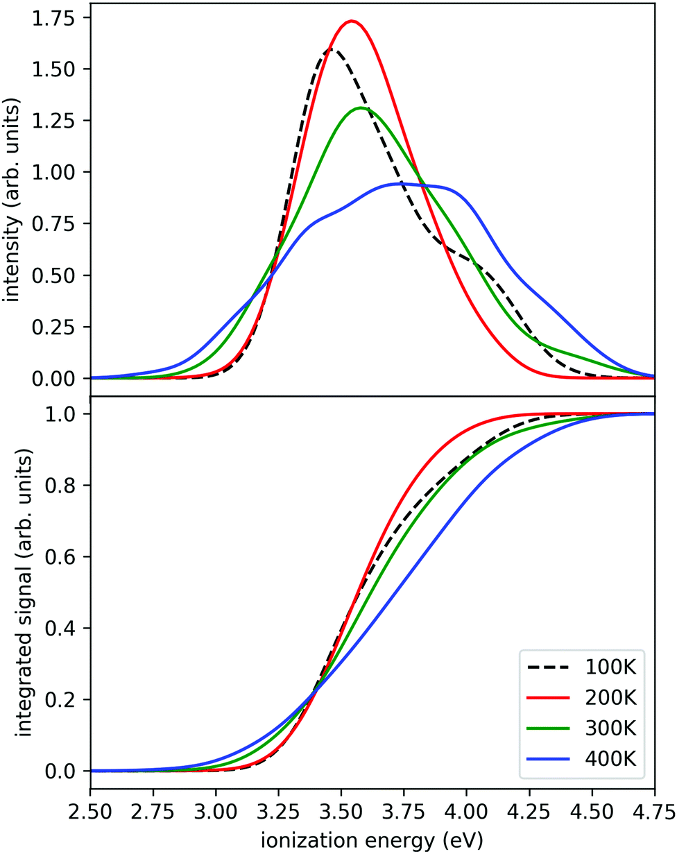 | ||
| Fig. 3 Simulated ionization probabilities (upper panel) and their integral (lower panel) for Na(H2O)7 at different temperatures. The ionization probabilities are linked to the temperature dependent degree of sodium solvation. At low energies ion pairs are found, at high energies the sodium atom remains intact. | ||
4 IR-UV delay time dependence of the ion signal
In the previous section we have illustrated the strong effect of cluster temperature on the abundance of sodium–water clusters with ionization energies in the onset region of the ion yield curve below 3.5 eV. This behaviour we exploit to measure IR-spectra based on the ion signal increase by IR photon absorption before photoionization, see e.g.ref. 28, 29 and 64. From the findings described e.g. in ref. 16 and 24 it is clear that the Na–water clusters are not stable at temperatures above 150 K due to evaporative cooling. However, the monomer ejection is a highly temperature sensitive process, depending strongly on the time scale of the experiment. Before the interaction with the laser light this period is around or below 1 ms depending on the beam velocity. Because the evaporation rates strongly decrease when cluster temperatures approach 150 K24 the evaporation effect has not been taken into account in the temperature analysis of Section 2. Clearly, the maximum temperature in our experiment can be higher than the 145 K, reported as the evaporative cooling limit in ref. 16 because the corresponding experiment is performed on a timescale in the range of seconds. The simulations in the section above indicate a very high sensitivity of the IR signal on cluster temperature above 200 K. Therefore it can be expected to trace the evaporative cooling process in the time evolution of the ion signal when the clusters are heated well above 200 K within a few nanoseconds by the IR laser pulse. But there is another effect. The cluster size distribution will be changed by the IR multi-photon dissociation (IRMPD) process which is a more direct manifestation of evaporative cooling. Fortunately, this effect can be observed independently at negative IR-UV-delay times, which means that the clusters are first photoionized and then irradiated with the IR laser. The decisive difference of the two cases, the one with positive and the one negative delay times, is the absence of the Na 3s electron after photoionization, which is here connected to experiments with negative delay times. In this case the temperature effect on hydrated electron formation is absent. We observe in the experiment the pure thermal effect on the cluster size distribution. In this mode the experiment resembles more IRMPD experiments which use negative signals like the experiments on the water nonamer melting presented above in Fig. 2. We examined both effects, the isolated IRMPD based change of the size distribution at negative delay times and the coupling of evaporative cooling and sodium solvation at positive delay times for two expansion conditions resulting in predicted cluster temperatures of 154 K (Argon expansion) and 70 K (helium expansion), which are the second helium and the first argon case in Table 4. The clusters are irradiated at 3400 cm−1 in the region of maximum absorption for amorphous clusters, which is largely independent of cluster size until crystallization begins, see e.g.ref. 21 and 28. The results are shown in Fig. 4.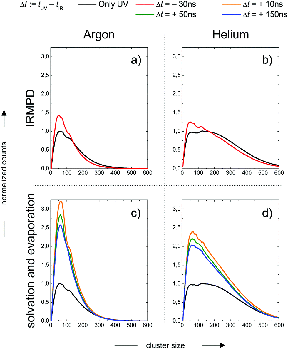 | ||
| Fig. 4 Cluster size distribution as a function of the IR-UV-delay time for two expansion conditions. Upper panels: Photoionization before IR excitation, absence of the Na 3s electron, pure thermal IR-multiphoton dissociation (IRMPD) effect on the measured size distribution at negative delay times. Lower panels: IR excitation before photoionization, presence of Na 3s electron, coupled Na solvation and evaporative cooling effect on the measured size distribution at positive delay times. Expansion conditions Argon (left panels): Estimated final cluster temperature 154 K (see Table 5). Expansion conditions Helium (right panels): Estimated final cluster temperature 70 K (see Table 5). | ||
In the upper panels we observe a shift in the size distribution to smaller sizes. It is more pronounced for the Argon seeded expansion. The comparison of the IRMPD effect with the sodium solvation effect in the the lower panels of Fig. 3 shows remarkable differences. First, the depletion of cluster abundance under IRMPD conditions for larger cluster sizes is not observed at positive delay times. Second, the signal increase due to sodium solvation is much stronger than the IRMPD effect on the size distribution. Third, the IR signal is time dependent only at positive delay times, for the constancy at negative delay times see Fig. 7.
These observations allow for several interpretations and conclusions. First, the signal increase caused by sodium solvation in the heated and most likely liquefied clusters is the clearly dominating effect in our experiment; it is present over the complete size distribution. Second, the time dependent signal loss shows exponential behaviour. It is stronger within the shorter interval from 10 to 50 ns compared to 50 to 150 ns (in this time window the two lasers fully overlap, see Fig. S5 in the ESI†). Third, this signal loss we attribute to an indirect effect of evaporative cooling, the diminished abundance of highly solvated sodium 3s electrons with low ionization energies in the cooling clusters. Clear evidence for this interpretation is given by the homogeneous decay of the signal, especially in the lower size region where a signal increase is expected due to the isolated IRMPD effect (see upper panels of Fig. 4). We cannot rule out a minor contribution of the IRMPD effect to the time dependent IR signal, but it is clearly not the dominating effect. This issue will be further inspected below in a simulation of the time dependence of the evaporation process. Furthermore, we find that the achievable signal increase in the range of factors of 2 to 3 is in line with the predicted ion yield increase at 3.2 eV for an temperature rise to 300 K (see lower panel of Fig. 3). However, one may argue that the cluster size of n = 7 is too small to interpret the much larger clusters examined in the experiment. As indicated above, it is known from the pioneering work of Hertel and co-workers that the ionization energy of Na–water clusters has almost dropped to limit for large clusters at n = 4.54 Furthermore, our detailed analysis of the photoionization spectra in the the size range up to n = 100 revealed some subtle changes with regard to the high energy end of the ion yield curve; but they clearly showed very similar shapes for n = 7 and larger clusters32 in the 3 to 3.5 eV region, which is probed here. The extensive work of many groups on this issue (see e.g.ref. 29 and literature cited therein) has shown that the sodium solvation is a rather local phenomenon at the cluster surface explaining the very weak scaling of the ionization energy with cluster size11,32 which is different to Na ammonia clusters and water clusters with excess electrons.65–67 To get some more information about the expected temperature change (in the first 200 ns after the rapid IR laser heating and in the flight time until detection in the mass spectrometer) and to analyse the effect of the different starting temperatures of around 70 and 154 K, we have built a simple simulation set-up. For evaluating the time evolution of cluster temperatures we take the data used in Section 2 for heat capacities and water binding energies. The temperature and size dependent evaporation rates are taken from the study by Borner et al.,68 see also the early work of Näher and Hansen.69 We use the UV only spectrum as start configuration and we evaluate the effect of water monomer loss on cluster size and temperature, which are closely coupled. In the simulation the clusters move in sufficiently small time steps of 1 to 10 ns in a size and temperature matrix to smaller sizes and lower temperatures. This movement is slowed down in time by the decreasing evaporation rates at lower temperatures. More information on the simulation are given in the ESI.† In Fig. 5 the simulated effect of this process on the size distribution of the Argon experiment in Fig. 4 is shown as a function of the initial temperature.
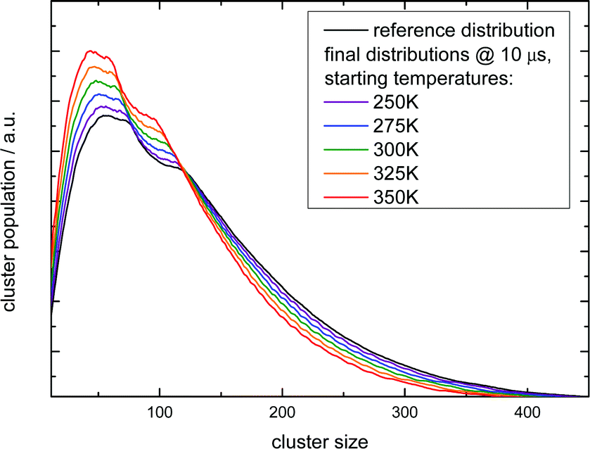 | ||
| Fig. 5 Simulation of the IR multi-photon dissoziation effect on the cluster size distribution as a function of the temperature rise when they are irradiated with an IR pulse after photoionization. The simulations model the experiment shown in the left upper panel of Fig. 4. The experimental conditions belong to the first Argon experiment in Table 4. | ||
The simulation time is 10 μs which is in the range of the flight time in the reflectron mass spectrometer before the clusters are detected. However, this must be an estimated average time scale with regard to fragmentation in the acceleration zone, in the drift region and in the reflectron zone, see e.g.ref. 27. Nevertheless, the simulation time is quite insensitive for longer simulation runs (longer then 1 microseconds) because in temperature range of 200–225 K monomer evaporation becomes very slow. To see a further temperature drop the simulation time must be extended to milliseconds and seconds, but this cannot be probed in a reflectron time of flight mass spectrometer. Compared with the experiment (left upper panel of Fig. 4) the simulated increase of abundance below n = 100 is stronger than the depletion at larger sizes. However, we have to keep in mind that the IR laser is tuned to 3400 cm−1 while the absorption maximum in this experiment gradually shifts to 3220 cm−1 as the clusters start crystallizing around n = 90.15 Therefore larger clusters are heated less effectively explaining the weaker experimental IRMPD effect in the upper size range. We note here that this is an independent indicator for the early onset of crystallization in this experiment. The comparison with the simulation indicates a cluster temperature of above 300 K after IR heating at lower sizes and rather around 300 K for the larger sizes. Furthermore, we have to take into account again the remaining methodological challenges for accurately predicting evaporation rates of water clusters, see ref. 68 and 70. Nevertheless, in qualitative terms we arrive at a consistent picture. The same is true when we examine the helium experiment for which the IRMPD effect is weaker. This is in line with the much lower temperature before the interaction with the IR laser light (70 K for He and 154 K for Ar) which should result in a lower temperature after the IR laser pulse. Furthermore the integral of the two curves is here almost the same (as it is in the simulation) because fully crystalline clusters are only observed above n = 400 at the tail of the distribution.28 The in this case homogeneous IRMPD signal again supports the IR-spectroscopic assignment. We note that the same IR laser energies and optical adjustments are used for the two experiments and that the signal to noise is high when we measure and plot the smoothed envelope of the size distribution. The same difference in the effects of IR heating we see for the signal increase at positive delay times in the lower panels of Fig. 4. As stated above, the general signal increase is in line with the simulation results of Section 3, but again the IR action effect is stronger for the Argon experiment with the higher starting temperature. Furthermore, the signal decrease at longer delay times is also stronger for the Argon experiment. Such an effect may be expected when we look at the simulated temperature and cluster size evolution for (H2O)100 in the first 200 ns, which is shown for several starting temperatures in Fig. 6.
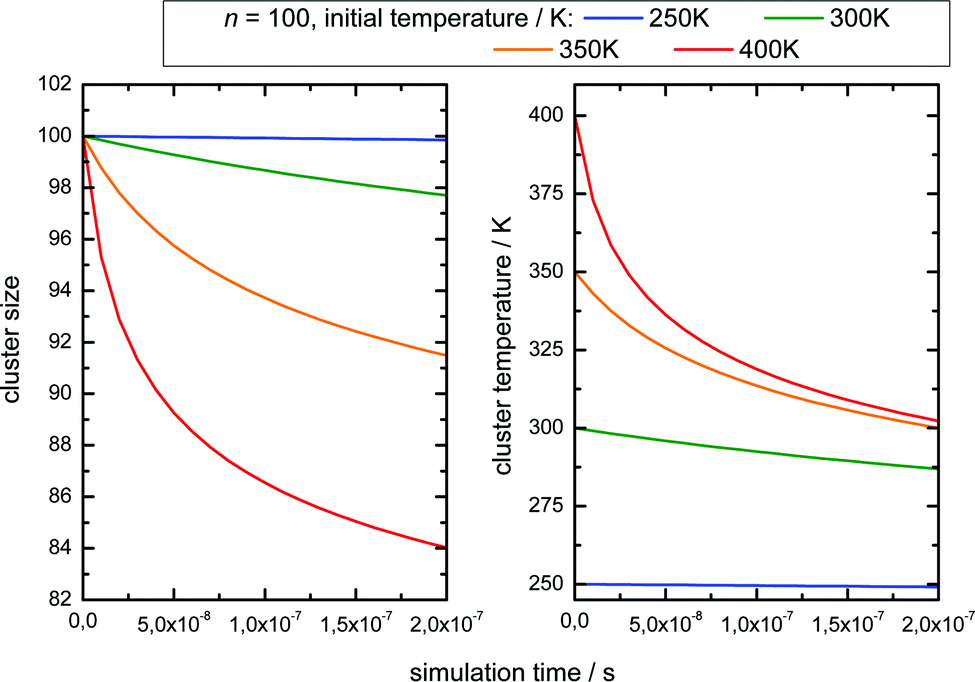 | ||
| Fig. 6 Simulation of monomer loss (left panel) and temperature drop (right panel) of (H2O)100 over 200 ns as a function of starting temperature. The sizes and temperature are weighted means of the distribution. | ||
Here we see that above 300 K the monomer loss and temperature decrease is significantly enhanced. This seems to correlate with the stronger signal drop in the Argon experiment (see lower panels of Fig. 4) which features a higher temperature before and after IR laser heating. However, we have to keep in mind that the observed signal decrease is not the direct effect of the temperature decrease but the coupling of it with sodium solvation and this may be more sensitive at temperatures below 300 K (see Fig. 3). Nevertheless, we can assume that the cluster temperature does not drop significantly below 250 K in first 200 ns because the evaporation dynamics are almost frozen at this temperature for this time scale. The experimental ion signal at 200 ns is clearly much nearer the maximum value than the baseline indicating a high degree of sodium solvation in line with results of Section 3. The semi-quantitative picture we get from the experiment and the simulations is that the clusters are heated well above 250 K by the IR laser pulse in both experiments of Fig. 4. And we see that the initially higher cluster temperature in the Argon experiment leads to stronger action effects which can be explained by the higher final temperature: on the longer time scale we see a stronger IRMPD effect while we observe in the first 200 ns a more pronounced signal increase and decay for the “warmer” Argon experiment. Vice versa the opposite effect of lowering the initial temperature can of course be produced by reducing the IR laser pulse energy or by tuning the IR laser frequency to regions with lower IR absorption. However, the situation becomes more complicated when geometry changes occur during the multi-photon absorption process. This should be expected when we look at the example of the water nonamer in Fig. 2. We have explored this effect for the helium experiment in the size range where crystalline spectral features become dominant.28 The results have important implications for the method and are discussed in the next section.
5 Implications for the method
We studied the temporal evolution of the ion signal for the second helium experiment of Table 4 at two IR laser frequencies, near the maximum absorption of crystalline clusters at 3200 cm−1 and near the maximum absorption of amorphous clusters at 3400 cm−1. The analyzed size range is the transition region, in which the IR spectra change from amorphous to dominating crystalline features.21,28 The results are shown in Fig. 7. | ||
| Fig. 7 In the two experimental traces shown in this figure we compare the IR-UV-delay time dependent effect of IR excitation of two different water cluster modes, one mode is the crystalline band at 3200 cm−1, the other mode is the band of amorphous clusters excited at 3400 cm−1. Different to the color coding of Fig. 4 we plot the IR signal as a function of the delay time. Both IR signal traces are limited to the amorphous-crystalline transition region of the size distribution (n = 300 to 400); the reason for the stability of the 3200 cm−1 trace is discussed in the text. The expansion conditions are those of the helium experiment in Fig. 4. | ||
At short delay times we see a similar IR signal at both IR frequencies which is expected for the amorphous–crystalline transition region. The temporal trends, however, are very different. The trace for the experiment at 3400 cm−1 shows the signal drop expected from the results shown in Fig. 4 for the whole size distribution. The experiment at 3200 cm−1 is different, here, within the experimental uncertainty, we cannot observe a signal drop in the first 150 ns. To understand this difference we have to consider geometry changes during the multi-photon absorption process. From previous studies48 it can be expected that the clusters in this size range are liquid above 180 K and they should relax to equilibrium geometries below the ns second time scale. This is in line with the simulations in Section 3 and the observation that we cannot delay the signal increase around 0 ns even at very low IR pulse energies. Therefore we have to assume that the geometry changes to liquid-amorphous structures above 180 K48 during the IR laser pulse of 10 ns and the IR spectra accordingly. As the 3200 cm−1 crystalline band disappears upon melting, further heating above 200 K is much less efficient due to the much lower IR absorption of amorphous clusters at 3200 cm−1. This effect is nicely illustrated by the melting of the nonamer in Fig. 2. The band at 3100 cm−1 is not present at 186 K and the absorption cross section has dropped to roughly one third. The effect for the IR excitation at 3400 cm−1 is the opposite. The crystalline clusters have significant absorption at 3400 cm−1 and upon melting the IR absorption would increase. We think that the effects we observe here are closely related to the transparent bands in IRMPD experiments, where weak hydrogen bonds may break after the first IR photon absorption and the action effect is suppressed for such a band (see e.g. the discussion in ref. 71). In the Na–water cluster case this effect has a very beneficent consequence. The clusters can be heated into a temperature range around or slightly above 200 K in which the positive signal of sodium solvation is triggered but the cluster dissociation is suppressed. In the first 200 ns this seems to be the case even at 250 K (see Fig. 6). The following near threshold photoionization may even stabilize the then cationic clusters because the photoionization constraints may demand thermal energy in the neutral clusters to surmount the ionization threshold.64 The combined effects can suppress IR and UV induced dissociation/fragmentation and allow for taking size selective IR spectra as demonstrated for n = 3 and n = 20.30,31 These studies were performed at reduced IR laser pulse energies (6 to 8 mJ) while we use high pulse energies around 10 mJ in this work to maximize the effects. These assignments rely on characteristic DAA features in the low frequency range of the IR spectrum of highly ordered water clusters (see Fig. 2) which are tagged with an external sodium atom. The onset of melting triggers the IR signal and blocks the characteristic band and thus reduces further heating. In principle this mechanism can be applied to other sodium doped, hydrogen bonded clusters,27,72 when solvated electrons are formed. However, this is not the case for nitrogen containing solvents73–75 and probably other clusters, where the scavenging of the sodium 3s electron by molecules with high electron affinity occurs. There is another important feature in Fig. 7. The delay time independent negative IRMPD signal at negative delay times is much stronger at 3400 compared to 3200 cm−1. Without the sodium solvation effect the temperature rise determines the depletion signal strength. And this signal is limited for crystalline clusters when they melt during the IR irradiation. In consequence the crystalline band is transparent in the IRMPD mode of our experiment. This mechanism may explain the observation of purely amorphous clusters in the first IRMPD experiments with ionic water clusters at n = 250.17 Finally, we would like to note that for both methods discussed here, the IRMPD approach and the IR spectroscopy with sodium doped water clusters, the number of photons absorbed in a multi-photon absorption process is important. In our method the onset of sodium solvation is the crucial point. This starts at around 200 K (see Section 3 and e.g. the simulations in ref. 48). In the IRMPD method the crucial point for the signal is the onset of monomer evaporation. This is still quite ineffective at 250 K as the simulations of Fig. 5 have shown. To trigger the IRMPD signal higher cluster temperatures (and more IR photons) or a much longer time scale are needed compared to our method.
6 Conclusions
In this work we have examined the temperature evolution of water clusters in IR action spectroscopy experiments using continuous supersonic expansions. We present an energy balance model that provides for a wide range of expansion conditions cluster temperatures in good agreement with independent spectroscopic indicators and detailed numerical simulations. This temperature information is used to analyze the time evolution of the ion signal in our IR action spectroscopy experiment based on changes in Na atom solvation and on the evaporative cooling effect. We find that the observed rapid signal increase within 5 ns is consistent with ab initio simulations of the temperature dependent shift in the low energy part of the photoionization spectrum of Na(H2O)7. This positive signal is much stronger than the independently studied IR multi photon dissociation effect on the size distribution. Increasing the IR UV delay time to 200 ns results in an exponenential signal decrease. On the basis of a direct molecular simulation we attribute both effects to the temperature decrease through evaporative cooling. The rapid decrease in the first 200 ns is coupled to changes in Na atom solvation, consistent with the ab initio simulations in section 3, while the much weaker IRMPD effect is observed on the microsecond timescale at the end of the drift zone at the MCP detector. The analysis further reveals reduced evaporative cooling in the upper size range of the distribution where previous experiments showed the presence of crystalline clusters with a lower IR absorption. This is a new and independent indicator for the cooling rate sensitive onset of crystallinity in water clusters. Furthermore we find strong indications for geometry changes during the IR multiphoton absorption process. The results suggest that highly ordered clusters can be detected without fragmentation because their characteristic bands disappear (avoiding further heating) when sodium solvation is triggered in the melting cluster.Conflicts of interest
There are no conflicts of interest to declare.Acknowledgements
D. B. acknowledges support by the Verband der Chemischen Industrie, grant 104371. Thomas Zeuch thanks the Deutsche Forschungsgemeinschaft for support (grants ZE890 1-2 and 4-1, numbers: 143238629 and 400183980). We thank Steven Celik for his support in conducting the experiments. J. S. and P. S. were supported by Czech Science Foundation project number GA18-16577S, the computations were allowed due to the support by The Ministry of Education, Youth and Sports from the Large Infrastructures for Research, Experimental Development and Innovations project e-Infrastructure CZ-LM2018140.References
- G. Torchet, P. Schwartz, J. Farges, M. F. de Feraudy and B. Raoult, J. Chem. Phys., 1983, 79, 6196–6202 CrossRef CAS.
- U. Buck and F. Huisken, Chem. Rev., 2000, 100, 3863–3890 CrossRef CAS.
- N. I. Hammer, J. R. Roscioli, J. C. Bopp, J. M. Headrick and M. A. Johnson, J. Chem. Phys., 2005, 123, 244311 CrossRef.
- B. Bandow and B. Hartke, J. Phys. Chem. A, 2006, 110, 5809–5822 CrossRef CAS.
- R. W. Larsen, P. Zielke and M. A. Suhm, J. Chem. Phys., 2006, 125, 154314 CrossRef.
- R. W. Larsen, P. Zielke and M. A. Suhm, J. Chem. Phys., 2007, 126, 194307 CrossRef.
- T. Hamashima, K. Mizuse and A. Fujii, J. Phys. Chem. A, 2011, 115, 620–625 CrossRef CAS.
- K. R. Asmis and D. M. Neumark, Acc. Chem. Res., 2011, 45, 43–52 CrossRef.
- A. Fujii and K. Mizuse, Int. Rev. Phys. Chem., 2013, 32, 266 Search PubMed.
- J. A. Fournier, C. J. Johnson, C. T. Wolke, G. H. Weddle, A. B. Wolk and M. A. Johnson, Science, 2014, 344, 1009–1012 CrossRef CAS.
- A. H. C. West, B. L. Yoder, D. Luckhaus, C.-M. Saak, M. Doppelbauer and R. Signorell, J. Phys. Chem. Lett., 2015, 6, 1487–1492 CrossRef CAS.
- R. J. Cooper, M. J. DiTucci, T. M. Chang and E. R. Williams, J. Am. Chem. Soc., 2016, 138, 96–99 CrossRef CAS.
- S. Kazachenko and A. J. Thakkar, J. Chem. Phys., 2013, 138, 194302 CrossRef.
- N. Sugawara, P. J. Hsu, A. Fujii and J. L. Kuo, Phys. Chem. Chem. Phys., 2018, 20, 25482–25494 RSC.
- D. Moberg, D. Becker, C. W. Dierking, F. Zurheide, B. Bandow, U. Buck, A. Hudait, V. Molinero, F. Paesani and T. Zeuch, Proc. Natl. Acad. Sci. U. S. A., 2019, 116, 24413–24419 CrossRef CAS.
- C. Hock, M. Schmidt, R. Kuhnen, C. Bartels, L. Ma, H. Haberland and B. V. Issendorff, Phys. Rev. Lett., 2009, 103, 073401 CrossRef CAS.
- J. T. O'Brien and E. R. Williams, J. Am. Chem. Soc., 2012, 134, 10228 CrossRef.
- T. K. Esser, B. Hoffmann, B. Anderson and K. R. Asmis, Rev. Sci. Instrum., 2019, 90, 125110 CrossRef.
- J. Brudermann, U. Buck and V. Buch, J. Phys. Chem. A, 2002, 106, 453 CrossRef CAS.
- C. Steinbach, P. Andersson, M. Melzer, J. K. Kazimirski, U. Buck and V. Buch, Phys. Chem. Chem. Phys., 2004, 6, 3320–3324 RSC.
- U. Buck, C. C. Pradzynski, T. Zeuch, J. M. Dieterich and B. Hartke, Phys. Chem. Chem. Phys., 2014, 16, 6859–6871 RSC.
- N. Gimelshein, S. Gimelshein, C. C. Pradzynski, T. Zeuch and U. Buck, J. Chem. Phys., 2015, 142, 244305 CrossRef CAS.
- C. J. Tainter and J. L. Skinner, J. Chem. Phys., 2012, 137, 104304 CrossRef CAS.
- N. Gimelshein, S. Gimelshein, C. C. Pradzynski, T. Zeuch and U. Buck, J. Chem. Phys., 2015, 142, 244305 CrossRef CAS.
- T. Schindler, C. Berg, G. Niedner-Schatteburg and V. E. Bondybey, Chem. Phys. Lett., 1996, 259, 1137–1140 Search PubMed.
- C. Steinbach, M. Fárník, I. Ettischer, J. Siebers and U. Buck, Phys. Chem. Chem. Phys., 2006, 8, 2752–2758 RSC.
- R. M. Forck, C. C. Pradzynski, S. Wolff, M. Oncak, P. Slavicek and T. Zeuch, Phys. Chem. Chem. Phys., 2012, 14, 3004–3016 RSC.
- C. C. Pradzynski, R. M. Forck, T. Zeuch, P. Slavíček and U. Buck, Science, 2012, 337, 1529–1532 CrossRef CAS.
- T. Zeuch and U. Buck, Chem. Phys. Lett., 2013, 579, 1 CrossRef CAS.
- R. M. Forck, J. M. Dieterich, C. C. Pradzynski, A. L. Huchting, R. A. Mata and T. Zeuch, Phys. Chem. Chem. Phys., 2012, 14, 9054 RSC.
- C. C. Pradzynski, C. W. Dierking, F. Zurheide, R. M. Forck, U. Buck, T. Zeuch and S. S. Xantheas, Phys. Chem. Chem. Phys., 2014, 16, 26691–26696 RSC.
- C. W. Dierking, F. Zurheide, T. Zeuch, J. Med, S. Parez and P. Slavicek, J. Chem. Phys., 2017, 146, 244303 CrossRef.
- B. Wyslouzil and J. Wölk, J. Chem. Phys., 2016, 145, 211702 CrossRef.
- B. Schläppi, J. Litmann, J. Ferreiro, D. Stapfer and R. Signorell, Phys. Chem. Chem. Phys., 2015, 17, 25761 RSC.
- U. Buck and H. Meyer, Phys. Rev. Lett., 1984, 52, 109 CrossRef CAS.
- S. Schütte and U. Buck, Int. J. Mass Spectrosc., 2002, 220, 1887 CrossRef.
- C. Bobbert, S. Schütte, C. Steinbach and U. Buck, Eur. Phys. J. D, 2002, 19, 183 CAS.
- M. Fárník and J. Lengyel, Mass Spectrom. Rev., 2018, 37, 630–651 CrossRef.
- J. Brudermann, P. Lohbrandt, U. Buck and V. Buch, J. Chem. Phys., 2000, 24, 11038 CrossRef.
- J. Brudermann, PhD thesis, University of Goettingen, 1999.
- R. Jansen, I. Wysong, S. Gimelshein, M. Zeifman and U. Buck, J. Chem. Phys., 2010, 132, 244105 CrossRef.
- R. Jansen, N. Gimelshein, S. Gimelshein and I. Wysong, J. Chem. Phys., 2011, 134, 244105 CrossRef.
- D. R. Miller, Free jet sources, in Atomic and Molecular Beam Methods, University Press, Oxford, 1988 Search PubMed.
- U. Buck and F. Huisken, Chem. Rev., 2000, 100, 3863 CrossRef CAS.
- K. Liu, M. G. Brown and R. J. Saykally, J. Phys. Chem. A, 1997, 101, 8995 CrossRef CAS.
- C. Perez, M. T. Muckle, D. P. Zaleski, N. A. Seifert, B. Temelso, G. C. Shields, Z. Kisiel and B. H. Pate, Science, 2012, 336, 897 CrossRef CAS.
- C. J. Tainter and J. L. Skinner, J. Chem. Phys., 2012, 137, 104304 CrossRef CAS.
- J. C. Johnston and V. Molinero, J. Am. Chem. Soc., 2012, 134, 6650 CrossRef CAS.
- C. Steinbach and U. Buck, Int. J. Mass Spectrosc., 2002, 220, 183–192 CrossRef.
- U. Buck, R. Krohne and P. Lohbrandt, J. Phys. Chem., 1997, 106, 3205 CrossRef CAS.
- J. Brudermann, P. Lohbrandt, U. Buck and V. Buch, Phys. Rev. Lett., 1998, 80, 2821 CrossRef CAS.
- T. N. Wassermann and M. A. Suhm, J. Phys. Chem. A, 2010, 114, 8223–8233 CrossRef CAS.
- R. Forck, I. Dauster, Y. Schieweck, T. Zeuch, U. Buck, M. Oncak and P. Slavicek, J. Chem. Phys., 2010, 132, 221102 CrossRef.
- I. V. Hertel, C. Hüglin, C. Nitsch and C. P. Schulz, Phys. Rev. Lett., 1991, 67, 1767 CrossRef CAS.
- Y. Sugita and Y. Okamoto, Chem. Phys. Lett., 1999, 314, 141–151 CrossRef CAS.
- O. A. Vydrov and G. E. Scuseria, J. Chem. Phys., 2006, 125, 234109 CrossRef.
- S. Grimme, J. Comput. Chem., 2006, 27, 1787–1799 CrossRef CAS.
- I. Ufimtsev and T. Martinez, J. Chem. Theory Comput., 2009, 5, 2619–2628 CrossRef CAS.
- D. Hollas, J. Suchan, M. Ončák and P. Slavíček, PHOTOX/ABIN: Pre-release of version 1.1, 2018 Search PubMed.
- M. Ončák, L. Šištík and P. Slavíček, J. Chem. Phys., 2010, 133, 174303 CrossRef.
- F. Della Sala, R. Rousseau, A. Görling and D. Marx, Phys. Rev. Lett., 2004, 92, 183401 CrossRef.
- A. D. Boese and J. M. L. Martin, J. Chem. Phys., 2004, 121, 3405–3416 CrossRef CAS.
- M. J. Frisch, G. W. Trucks, H. B. Schlegel, G. E. Scuseria, M. A. Robb, J. R. Cheeseman, G. Scalmani, V. Barone, B. Mennucci, G. A. Petersson, H. Nakatsuji, M. Caricato, X. Li, H. P. Hratchian, A. F. Izmaylov, J. Bloino, G. Zheng, J. L. Sonnenberg, M. Hada, M. Ehara, K. Toyota, R. Fukuda, J. Hasegawa, M. Ishida, T. Nakajima, Y. Honda, O. Kitao, H. Nakai, T. Vreven, J. A. Montgomery, Jr., J. E. Peralta, F. Ogliaro, M. Bearpark, J. J. Heyd, E. Brothers, K. N. Kudin, V. N. Staroverov, R. Kobayashi, J. Normand, K. Raghavachari, A. Rendell, J. C. Burant, S. S. Iyengar, J. Tomasi, M. Cossi, N. Rega, J. M. Millam, M. Klene, J. E. Knox, J. B. Cross, V. Bakken, C. Adamo, J. Jaramillo, R. Gomperts, R. E. Stratmann, O. Yazyev, A. J. Austin, R. Cammi, C. Pomelli, J. W. Ochterski, R. L. Martin, K. Morokuma, V. G. Zakrzewski, G. A. Voth, P. Salvador, J. J. Dannenberg, S. Dapprich, A. D. Daniels, Farkas, J. B. Foresman, J. V. Ortiz, J. Cioslowski and D. J. Fox, Gaussian’09 Revision E.01, Gaussian Inc, Wallingford CT, 2009 Search PubMed.
- C. Steinbach and U. Buck, J. Phys. Chem. A, 2006, 110, 3128–3131 CrossRef CAS.
- C. Steinbach and U. Buck, J. Chem. Phys., 2005, 122, 134301 CrossRef CAS.
- A. Kammrath, J. R. R. Verlet, G. B. Griffin and D. M. Neumark, J. Chem. Phys., 2006, 125, 076101 CrossRef.
- L. Ma, K. Majer, F. Chirot and B. von Issendorff, J. Chem. Phys., 2009, 131, 144303 CrossRef.
- A. Borner, Z. Li and D. A. Levin, J. Chem. Phys., 2013, 138, 064302 CrossRef.
- U. Näher and K. Hansen, J. Chem. Phys., 1994, 101, 5367–5371 CrossRef.
- P. Varilly and D. Chandler, J. Phys. Chem. B, 2013, 117, 1419–1428 CrossRef CAS.
- T. I. Yacovitch, N. Heine, C. Brieger, T. Wende, C. Hock, D. M. Neumark and K. R. Asmis, J. Phys. Chem. A, 2013, 117, 7081–7090 CrossRef CAS.
- R. Forck, I. Dauster, U. Buck and T. Zeuch, J. Phys. Chem. A, 2011, 115, 6068–6076 CrossRef CAS.
- J. Lengyel, J. Kočišek, V. Poterya, A. Pysanenko, P. Svrčková, M. Fárník, D. Zaouris and J. Fedor, J. Chem. Phys., 2012, 137, 034304 CrossRef CAS.
- D. Šmídová, J. Lengyel, A. Pysanenko, J. Med, P. Slavíček and M. Fárník, J. Phys. Chem. Lett., 2015, 6, 2865–2869 CrossRef.
- J. Lengyel, A. Pysanenko, P. Rubovič and M. Fárník, Eur. Phys. J. D, 2015, 69, 269 CrossRef.
Footnotes |
| † Electronic supplementary information (ESI) available. See DOI: 10.1039/d0cp05390b |
| ‡ Now at: Lonza Solutions AG, 3930 Visp, Switzerland. |
| This journal is © the Owner Societies 2021 |