 Open Access Article
Creative Commons Attribution 3.0 Unported Licence
Relaxometry models compared with Bayesian techniques: ganglioside micelle example†
Pär
Håkansson

NMR Research Unit, University of Oulu, P.O. Box 3000, 90014 Oulu, Finland. E-mail: par.hakansson@oulu.fi
First published on 5th January 2021
Abstract
In this work a methodology to perform Bayesian model-comparison is developed and exemplified in the analysis of nuclear magnetic relaxation dispersion (NMRD) experiments of water in a ganglioside micelle system. NMRD is a powerful tool to probe slow dynamics in complex liquids. There are many interesting systems that can be studied with NMRD, such as ionic and lyotropic liquids or electrolytes. However, to progress in the understanding of the studied systems, relatively detailed theoretical NMRD-models are required. To improve the models, they need to be carefully compared, in addition to physico-chemical considerations of molecular and spin dynamics. The comparison is performed by computing the Bayesian evidence in terms of a thermodynamic integral solved with Markov chain Monte Carlo. The result leads to a conclusion of two micelle water-pools, and rules out both less and more parameters, i.e., one and three pools. On the other hand, if only the quality of the fits is considered (i.e., mean square deviation or χ2) a three water-pool model is the best. The latter can be expected since with more adjustable parameters a better fit is more likely. Bayesian evidence is needed to rank the uncertainty of the models, and in order to explain the outcome a notation of Ockham-entropy is defined. The two approximate selection tools, Akaike and Baysian information criterions, may lead to wrong conclusions compared to the full integration. This methodology is expected to be one of several important tools in NMRD model development; however, it is completely general and should find awakened use in many research areas.
1 Introduction
The measurement of relaxation rates of nuclear spins versus resonance frequency is typically denoted as relaxometry and the recorded data form a relaxation dispersion (NMRD) profile. The experiment typically covers kHz to MHz resonance frequency and adds additional information to NMR spectroscopy (denoted as NMR relaxation). In particular, relaxometry can characterise the dynamics in a wide range from the nano- to micro-second regime.1 These properties open the way to study complex systems such as cement, petroleum fluids, biological tissue and collective motion of whole proteins,2 and dynamics in liquid crystals.3To obtain more meaningful information from relaxation experiments, relaxation models are utilized to provide details of the mechanisms underlying spin relaxation.4 Starting from the spin-system under study, the relevant mechanism may involve dipole–dipole, chemical exchange, paramagnetic and quadrupole contributions,5–12 as well as chemical shift anisotropy.13
The challenges in building models involve the incorporation of consistent molecular dynamics processes to explain experimental observations and account for spin-dynamics with sufficient accuracy.14–16 Hence, these challenges may come in the form of (i) multiple physical interpretations and (ii) more than one parametrization within a specific physical picture. By addressing (i) and (ii), the relaxometry-research community can strengthen the communication of results and make progress in model development for challenging systems.
Bayesian model selection is expected to provide a powerful method to rank conclusions drawn from different models and thus navigate past the challenges. Hence, in light of the data, NMRD-profile and additional experiments such as NMR-relaxation, diffusion and X-ray, we can determine the “best” model out of several competing proposals. The definition of “best” needs to include more than minima of cost functions like χ2.17 Rather, it should focus on the reproducibility and a balance quality of fit versus uncertainty due to the multitude of parameters to be determined.18
Model selection is expected to help in navigating the physics and chemistry underpinning the relaxation models. This goes beyond the qualitative guide for model selection via Ockham's razor, which may be formulated as “it is futile to do with more what can be done with fewer”.19
For the water study in this work, the proton dipole–dipole (DD)-relaxation is the most important mechanism to model. Even for one mechanism, multiple relaxation pathways can prove important, such as intramolecular contribution,20 intermolecular DD modulated by molecular diffusion,21,22 and/or proton exchange.23 The vast majority of relaxometry studies merge relevant physics in an analytical model describing the dynamics of the system and lead to a relatively large set of adjustable parameters.5 Ideally a signature NMRD feature can be used and strengthen the model interpretation with fewer parameters such as DD-relaxation enhancement.11 Such pronounced features are explored for paramagnetic10,16 super-paramagentic24 and quadrupole spin-systems.25,26
In this work the methodology is provided for Bayesian model selection and tested on micelle NMRD data.5 In particular the parametrization for a class of models (noted as (ii) above), addresses the question: why does the two water-pool model give the best explanation of data and not a simpler or more complex model? Hence, does the data support this more complex model?
The communication can thus be strengthened, especially towards researchers who are not experts in this field. Other research-fields such as astrophysics and cosmology have a long tradition of using and benefiting from these methods.27,28
A deeper understanding of approximations in analytical models as well as a partial or complete reduction of adjustable parameters has been obtained with molecular dynamics simulations. In relaxometry studies, this is achieved for paramagnetic relaxation enhancement,29 rotation and translation of small molecules,30 water at the bilayer interface,8 water in cement,31 and ionic liquids,13 lyotropic phases,14,32 porous organic cages7 and proteins.33 The simulation studies opens a way to explore the validity of analytical models and for some systems serves as the method of choice. However, model comparisons are not removed by using molecular dynamics simulations; instead, questions such as what is the sufficient size and timespan as well as what forcefield or quantum-chemistry methods are sufficiently accurate arise. Hence, based on different types of simulations, what outcome is the best in describing NMR-relaxation/relaxometry?
The estimation of model parameters and model comparison is centred around a cost function such as χ2:
 | (1) |
There are large sets of tools proposed around cost functions to compare models; the reduced χ2 can be computed by dividing by N − k and for instance over-fitting can be proposed. However, in particular for nonlinear models we don't know how many degrees of freedom are present and the guess “N − k”, where k is the number of parameters, is not robust.35 Hence, the χ2-value does not allow for model comparison in general.
Two approximate routes: the Akaike information criterion (AIC) and the Bayesian information criterion (BIC), both attempt to balance quality of fit with complexity of the model. These methods have as one assumption an asymptotic limit of N for a reduced error.36 In recent work these have been tested and found to have limited value in NMRD micelle studies.
The cross-validation (analysing part of the data) or more generally the Bootstrap-sampling have the drawbacks that the validity is in the asymptotic limit17,37 and for model comparison, only approximate forms are provided.36,38 Given the common situation of a small data set (N) in NMR-relaxation and NMRD the bootstrap method will not be explored in the current work.
In this work we follow instead Bayesian theory and compute the model evidence, which combines uncertainty due to a multitude of adjustable parameters and the quality of fit. Thus, a quantitative tool corresponding to Ockham's razor is obtained.36,39,40 A path to understand Bayesian evidence is assisted by identifying and defining Ockham-entropy in this work, since suitable terms to discuss the results are lacking.18
Bayesian evidence is a challenging high-dimensional integral to compute even with Monte Carlo methods. However, by introducing a thermodynamic integration the sought property is computed with multiple but vastly less demanding Markov chain Monte Carlo (MCMC) methods.41 In this work we implement thermodynamic integration and show that this is a computationally feasible route for relaxometry model comparison. The result is quantitative discrimination between models combining quality of fit and penalising over parametrization with Ockham-entropy.
In this paper, the relaxation model derived in previous work5 is presented in Section 2. In Section 3, the relevant Bayesian theory is provided with discussion of the introduced Ockham-entropy. This is followed by aspects to consider in MCMC simulations and the code is discussed in Section 4. Finally the NMRD example is analysed and presented in Section 5, followed by a summarising conclusion in Section 6.
2 Relaxation model
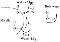
In this work we reexamine and follow closely the notation for the model presented in ref. 5, and refer to this work for further model discussions. The experimental observation of longitudinal relaxation rate Rexp1(ω0) is the rate-of-change in the spin ensemble due to the influence of the environment at resonance frequency ω0. At relatively low fields the dominating relaxation pathway is the DD-mechanism where the relaxation matrix for pairwise DD-coupling is well documented in the literature.4,23The key to the relaxation study5 is the formulation of a relevant physical picture, i.e. the two water-pool model depicted in Fig. 1. The two types of waters are denoted (βi, i = 1, 2) both located at the micelle. Reasons for more than one pool may be due to the large ganglioside head-group allowing for several water locations, leading to different exchange times (τw,i) and populations (fβi), but modulation by the same overall micelle rotation τR. The non-bound waters are denoted as bulk water in Fig. 1. In addition there are 2–3% ganglioside protons that are not addressed with the model.5
The theoretical prediction (RT1(ω)) takes the form
| RT1(ω) = α + fβ1R1,β1(ω) + fβ2R1,β2(ω) | (2) |
 | (3) |
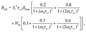 | (4) |
 | (5) |
2.1 Proposed models
The intra-molecular DD-amplitude may be determined from | (6) |
Relaxometry experiments are less sensitive to some model aspects and it makes sense to reduce the number of determined parameters. Following ref. 5, the product Si2fβi is estimated, together with τc,i and α. Thus, the two water-pool model contains five adjustable parameters per temperature5x = {α,Si2fβi,τc,i}, (i = 1, 2) and 15 in total.
We can not tell in advance how many water-pools there actually are, and more importantly, how many the NMRD experiments are sensitive to. This opens up a qualitative discussion along the line of Occham's razor to motivate a suitable number of water-pools, two in the original work.5 The number of water-pools, however, forms a transparent example where quantitative model comparison may be followed. Thus we consider the models Ma, Mb and Mc with two, one and three water-pools, respectively, leading to the number of adjustable parameters being: ka = 15, kb = 9 and kc = 21.
The results are discussed in terms of Stokes–Einstein–Debye (SED) relation and furthermore, a challenge is observed in extracting temperature dependence in (Si2fβi). These aspects motivate a two-pool model Md with a reduced set of parameters (kd = 10) explicitly including SED and with a constant parameter (Si2fβi).
As pointed out,5 modelling can be refined if we have complementary heavy water experiments.43 Furthermore, classical molecular dynamics may propose individual values to the merged (Si2fβi) parameter,44 and quantum chemical molecular dynamics may suggest constraints on proton exchange times. High field T1 measurement increases the spanned frequency range with one order of magnitude. Hence, the model comparison is evolving and needs to be open to new information.
3 Theory: Bayesian approach to model selection
To define the model selection, consider the probability of model Mj in the light of available data Rexp (in this work the NMRD profile) that is formulated with Bayesian theory. With the given (additional) information I (for instance known concentration of surfactants, temperature of experiments, etc.)41 the probability takes the form | (7) |
 | (8) |
 | (9) |
3.1 Thermodynamic integration
For many problems, eqn (8) is a high-dimensional integral and is difficult to estimate with numerical methods.36,40 A flavour of the numerical challenge is given in Fig. 2 where the details of the structure of the likelihood function needs to be integrated.40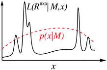 | ||
| Fig. 2 One-dimensional sketch illustrating the challenge with eqn (8), the likelihood function (L) in solid-black line and prior probability distribution of parameter (x) in dashed red line. The detailed structure of the likelihood function makes a high-dimensional integral challenging to compute by direct Monte Carlo sampling. | ||
By introducing a one-dimensional thermodynamic integral instead of attempting direct computation of eqn (8), a much less demanding problem is obtained. In fact, as exemplified,41 this may reduce the required number of sampling configurations from 10138 to 106! To compute eqn (8) as a thermodynamic integral (without introducing approximations) an auxiliary function is introduced:40,41
 | (10) |
![[thin space (1/6-em)]](https://www.rsc.org/images/entities/char_2009.gif) ln[F]/∂β = F−1∂F/∂β) is used. This gives:
ln[F]/∂β = F−1∂F/∂β) is used. This gives: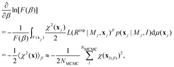 | (11) |
Integrating eqn (11) over [0,1] gives
 | (12) |
We note that in the limit β → 1 the integral in eqn (12) has a contribution from the quality of fit, hence, a smaller value of 〈χ2〉β=1 reduces the negative log or increases the model probability. The meaning of the complete integral in eqn (12) is addressed in what follows.
3.2 Entropy and model complexity
Although the integral of eqn (12) is a mathematic path to compute Bayesian evidence, it also provides an insight on its meaning, as seen from the reformulation: | (13) |
 | (14) |
By comparing eqn (13) and (14) we see that the integral in eqn (12) collects the entropy, or equivalently, the uncertainty in going from only prior to final parameter information, from the optimisation (or fit) of model to the experimental data. The (β = 1) contribution is lower since here the best information content is provided. Thus, a model is found that minimizes the β-integral but also maximizes the propability of the model [cf.eqn (7), simply considering log and non-log form]. With the entropy connection, just like a volume of ideal-gas compared with corresponding real-gas influences the entropy of a physical system, we can expect that the number of parameters, total volume, and extent parameters depend on each-other and also influence the entropy (cf.eqn (13)).
The literature proposes that Bayesian evidence consists of a best fit contribution and “model complexity”,18,19,28,36,39,40 however the correspondence and direct connection to entropy is not done. We find that for the physical chemistry community it is useful to define Ockham's entropy:
 | (15) |
3.3 Bayes factor
With two models proposed (Ma,Mb), eqn (12) enables the calculation of Bayes factor:36 | (16) |
2![[thin space (1/6-em)]](https://www.rsc.org/images/entities/char_2009.gif) ln[Bab] ln[Bab] |
Evidence against Mb |
|---|---|
| 0 to 2 | Just mention |
| 2 to 6 | Positive |
| 6 to 10 | Strong |
| >10 | Very strong |
3.4 Approximate model selection criteria
There are a number of approximate model selection criteria and we will explore the Akaike and Baysian information criterion, (AIC) and (BIC), respectivley:AIC = −2![[thin space (1/6-em)]](https://www.rsc.org/images/entities/char_2009.gif) ln(Lopt) + 2k, ln(Lopt) + 2k, |
BIC = −2![[thin space (1/6-em)]](https://www.rsc.org/images/entities/char_2009.gif) ln(Lopt) +k ln(Lopt) +k![[thin space (1/6-em)]](https://www.rsc.org/images/entities/char_2009.gif) ln(N), ln(N), |
![[thin space (1/6-em)]](https://www.rsc.org/images/entities/char_2009.gif) ln(Lopt) = χopt2 + “constant independent of model”. As for the full calculation provided in this work (see eqn (12)) BIC and AIC penalise a model with poor fit (large χ2) and excessive adjustable parameters, with expected
ln(Lopt) = χopt2 + “constant independent of model”. As for the full calculation provided in this work (see eqn (12)) BIC and AIC penalise a model with poor fit (large χ2) and excessive adjustable parameters, with expected ![[scr O, script letter O]](https://www.rsc.org/images/entities/char_e52e.gif) (N−1) error, of experimental data N.36
(N−1) error, of experimental data N.36
4 Methods
We present the parameter estimation with MCMC followed by the procedure for the thermodynamic integral (eqn (12)); for details we refer to the Matlab code and “readme” file presented in the GitHub example.46 It is noted that central to the study is the details of χ2 and thus the standard deviation (σi) of experimental relaxation rates in eqn (1). The experimental relaxation rates in the work of ref. 5 where obtained by fitting a function to Rexp data points, leading to a much too small standard deviation that was then calibrated with additional experiments. It is noted that the calibration factor of 10 for σi is used,5 corresponding in this work to a factor due to the normalization of 2 in this work (see eqn (1)).
4.1 MCMC parameter estimation
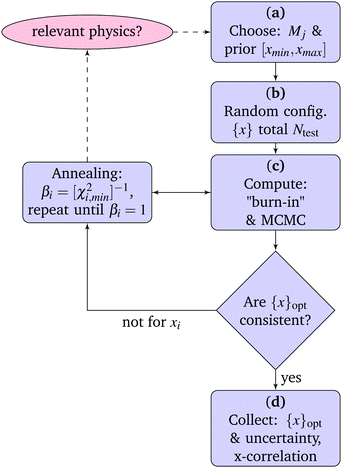
Before any work with model comparison, parametrization is needed. The ideas are implemented in Matlab/octave code46 and the steps are given in the flow-chart of parameter estimation (see Fig. 3). The start (a) for one of the models Ma,…,Md, the parameter prior (p(xj|Mj,I)) is chosen, that for this work is the uniform (uninformed) prior. For the user this involves setting the parameter-boundaries xmin and xmax (see Section 5). The choice of these ensures that parametrisation is reproducible within boundaries and no model is given extra advantage due to small interval. The parameter prior is used in (b) to generate Ntest starting configurations (in the range 4–10 {x}Ntest), where these parameter sets are random variables from the sought prior distribution.| T (°C) | τ c,1 (ns) | τ c,2 (ns) | α (s−1) | S 1 f β1 (10−3) | S 2 f β2 (10−3) |
|---|---|---|---|---|---|
| 10 | 157 | 11.6 | 0.64 | 0.25 | 1.6 |
| [144 168] | [6.6 18.6] | [0.58 0.69] | [0.23 0.27] | [1.1 2.6] | |
| 15 | 132 | 9.0 | 0.58 | 0.25 | 1.8 |
| [125 147] | [5.9 17] | [0.54 0.62] | [0.22 0.27] | [1.0 2.6] | |
| 20 | 123 | 9.6 | 0.53 | 0.23 | 1.6 |
| [115 135] | [6.4 17] | [0.49 0.57] | [0.20 0.25] | [0.9 2.3] | |
| x min ↔ xmax | 1.0 ↔ 1000 | 0.1 ↔ 100 | 0.001 ↔ 0.8 | 0.01 ↔ 100 | 0.01 ↔ 100 |
| T (°C) | τ c,1 (ns) | α (s−1) | S 1 f β1 (10−3) |
|---|---|---|---|
| 10 | 119 | 0.77 | 0.38 |
| [115 124] | [0.75 0.80] | [0.36 0.39] | |
| 15 | 102 | 0.70 | 0.37 |
| [99 107] | [0.69 0.72] | [0.36 0.39] | |
| 20 | 94 | 0.64 | 0.35 |
| [91 98] | [0.63 0.66] | [0.34 0.36] | |
| x min ↔ xmax | 1 ↔ 1000 | 0.001 ↔ 0.8 | 0.01 ↔ 100 |
| T (°C) | τ c,1 (ns) | τ c,2 (ns) | τ c,3 (ns) | α (s−1) | S 1 f β1 (10−3) | S 2 f β2 (10−3) | S 3 f β3 (10−3) |
|---|---|---|---|---|---|---|---|
| 10 | 183 | 49 | 4.5 | 0.58 | 0.18 | 0.3 | 3.5 |
| [153 215] | [17 70] | [1.2 40] | [0.1 0.65] | [0.13 0.24] | [0.23 0.85] | [1.8 12] | |
| 15 | 178 | 63 | 5.0 | 0.54 | 0.15 | 0.3 | 2.9 |
| [132 204] | [16 69] | [1.1 11.1] | [0.2 0.6] | [0.12 0.25] | [0.22 0.85] | [1.4 11] | |
| 20 | 140 | 40 | 2.5 | 0.39 | 0.16 | 0.31 | 5.0 |
| [122 192] | [15 69] | [0.8 7.9] | [0.1 0.54] | [0.08 0.22] | [0.17 0.85] | [1.7 13] | |
| x min ↔ xmax | 70 ↔ 1000 | 15 ↔ 70 | 0.1 ↔ 15 | 0.001 ↔ 0.8 | 0.01 ↔ 100 | 0.01 ↔ 100 | 0.01 ↔ 100 |
| T (°C) | R (Å) | τ w,1 (μs) | τ c,2 (ns) | α (s−1) | S 1 f β1 (10−3) | S 2 f β2 (10−3) |
|---|---|---|---|---|---|---|
| 10 | 49 | 8 | 11 | 0.64 | 0.24 | 1.7 |
| [48 50] | [2.1 10] | [9 16] | [0.61 0.67] | [0.23 0.26] | [1.3 2.0] | |
| 15 | — | — | 10 | 0.58 | — | — |
| [8 14] | [0.55 0.60] | |||||
| 20 | — | — | 9 | 0.54 | — | — |
| [7 12] | [0.51 0.56] | |||||
| x min ↔ xmax | 10 ↔ 100 | 0.001 ↔ 10 | 0.1 ↔ 100 | 0.001 ↔ 0.8 | 0.0 ↔ 0.1 | 0.0 ↔ 0.1 |
The core of MCMC is efficient sampling of configurations (c). For ease of introducing alternative prior distributions the current version, function MCMCstep.m,46 follows the Metropolis algorithm,7,47,48 hence, the proposed new parameter configurations are sampled in a random direction (not for instance guided by the likelihood function). Each parameter is given a move individually, following the Gibbs sampling algorithm.49 The parameter moves are reflected at the boundaries (xmin and xmax).
The acceptance ratio of steps should as a rule of thumb be ∼0.5 to efficiently probe lower probability regions but where higher value (shorter steps) leads to greater correlation between configurations. It is noted that more efficient sampling may be found, but these require model specific implementation.47 The step-length can be optimised versus the measured step correlation to further improve sampling. The step correlations are computed from the saved configurations, i.e., normalised auto and cross-correlation functions50 (see ESI† and implementation in the code46).
The step-lengths were determined by computing a sub-set of steps where the mean acceptance ratio is computed followed by calibration until within the interval [0.4, 0.6]. This was followed by ∼105 MCMC iterations towards equilibrium, the region of smallest χ2 (denoted “burn-in”). The burn-in is followed directly by attempt of productive MCMC-steps (∼106). The above sequence of steps is typically not intervened in by the user. At this point comes the main question of MCMC, have the configurations reached equilibrium? This question is addressed with a set of Ntest trajectories and looking for consistency in χopt2versus the standard deviation of χ2 (see Fig. S1 in ESI†). If some configurations remain in a local minimum, the annealing procedure is performed where simulations corresponding to higher “temperatures” (low β) are made and any local minima are more easily surpassed.
Obviously there is no global minimisation routine (MCMC or otherwise) capable of arbitrary complex models; thus if some very challenging problems occur, the user should also consider if the model represents relevant physics worth proceeding with.
With all the {x}Ntest configuration successfully completed (d) additional sets are computed up to and including the burn-in step, to verify that we have a reproducible global minimum in χ2. The results are summarised with xj-histograms, i.e. total density projected on each variable xj. Histograms are integrated to provide 95%-confidence intervals. The optimized parameters are in this work given by
 | (17) |
What is found valuable in the provided implementation46 is the ease by which calibration of the MCMC step-length is made automatic with the univariate moves (Gibbs sampling49). In addition, how random initial configurations converge by exploring a set of fixed annealing temperatures for the challenging cases. Challenges may appear for models with larger number of parameters that are still interesting to give a fair comparison. The annealing enables completely random initial configurations to query if the proposed model-result is reproducible within the given parameter boundaries.
There are several MCMC programs and it is found that in ref. 52 (used in NMRD53) the configuration move used is not transparent to the implementation including annealing. Furthermore, initial configurations are proposed to be from a “suitable starting point”.52 Such an approach does not work here where the goal is to probe the whole parameter volume as potential starting points.
4.2 Numerical thermodynamic integral
The numerical computation of the thermodynamic integral in eqn (12) is performed with the set of optimised configurations {xopt}Ntest (see Fig. 3) computing integrand at discrete β values. The discretization is found by starting from five β values with logarithmic discretisation on interval (0,1), where it is noted we have the β = 1 value from the parametrization and the β = 0 case is most efficient to generate with independently sampled configurations from the prior parameter distribution.Based on the integral computed with the trapezoidal rule,17 the interval with the largest contribution is located and split in half and the integral is recomputed. This procedure continues until the difference between two subsequent integrals is less than the desired tolerance. The same discretization was then used for all the models with β-values provided in the GitHub example.46
5 Results and discussion
The main aim of this work is to provide numerical (MCMC) Bayesian model selection to the relaxometry community and exemplify how this can be used in the interpretation of NMRD profiles. The example considered is relaxometry study of water in ganglioside Micelles,5 where previous work considers a model with two water-pools; this number (and not one, three or more pools) is deemed the feasible amount of information to extract from NMRD-profiles. The main question is if quantitative model selection can conclude how many pools is best with the given data.5.1 Model parametrization
From the parametrization of the models (Ma, Mb, Mc and Md) following Fig. 3 it is identified if any of the models provide exceptional challenges before continuing work with model comparison. The first stage, the parametrization, with optimal fits is provided in Fig. 5 and the estimated parameters in Tables 2–5, listing the parameter boundaries in the bottom rows.Common for models Ma to Md are that optimisation is performed globally over the 90 data points and the exploration of weight of inter-DD contribution case WD = 0.4. It was found5 that the model dependence of WD is weak and it is not the focus of this work to explore this further.
For model Ma it is found that MCMC estimation provide within 95%-confidence interval, χ2opt = 68 and largely, within the confidence interval, the same parameters as the original work,5 with data in Table 2.
Thus, the same physical interpretation5 is summarised, that is, a slow correlation time τc,1 dominated by overall rotational diffusion of ganglioside micelles; that from the Stoke–Einstein–Debye (SED) relation is consistent with the radius of 54 Å, concluded from measurements by other techniques.5 The shorter correlation time, originating from τc,2 (see Fig. 1) is ascribed to the proton exchange-modulated reorientation where water protons exchange with labile surfactant protons.5,54
The difference in the size of the confidence intervals is striking; for MCMC they are always larger where the difference for (S22fβ2) is a factor 50.5 Considering steps to check the MCMC parameter estimation, there are 7 simulations with random starting configurations within parameter boundaries (see range in Table 2). By estimating the MCMC-parameter auto-correlation (τsteps) a handle is obtained on how well the parameter space is sampled. It is found that χ2, (S22fβ2) and (S12fβ1) are sampled with 4 × 10⁴, 2 × 10² and 1 × 10³ correlation times, respectively. This points to a sufficiently sampled parameter-space given that additional “burn-in” is separately performed (see ESI,† Fig. S2).
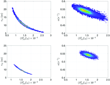
From the computed cross-correlations (see ESI†), a substantial amount is seen between (S22fβ2)–(τc,2) and (S22fβ2)–α for the 20 °C NMRD-profile and they are illustrated with histograms in the upper panels of Fig. 4. The parameter correlation explains the large error boundary found in MCMC estimation. Note that this in itself is not a problem for the MCMC-validity, except it leads to a large parameter uncertainty. This is since the whole parameter space is still sampled provided sufficiently long MCMC simulation is performed. On the other hand, for conventional fit-routine, parameter correlations introduce an error in confidence intervals since the parameter distribution is not known in that case.39
The parametrization of model Mb is given in Table 3 and Fig. 5 (χopt2 = 1346) assumes one water-pool. The model provides a poor description of high field data (see Fig. 5), however, the model is simpler with a total of 9 adjustable parameters. The least sampled parameter is (S12fβ1) with 6700 correlation times within the MCMC run and auto-correlation (for each parameter in MCMC run) is in the same regime as cross-correlations. The correlation time τc,1 is about 20% shorter than for model Ma and corresponds to a micelle radius about 3 Å smaller with the correlation time interpreted in terms of SED.
For model Mc, the parametrization is provided in Table 4 and the best fit in Fig. 5 (χopt2 = 18) where three water-pools are assumed, is also the best of all models tested. However, it is noted that this χopt2 is more than a factor of three lower than the number of experimental data-points, indicating an overfit of data. The parameter boundaries (τc,2 and τc,3) are chosen to be relatively narrow (based on the Ma result), in order for the study to be reproducible from random initial parameter configurations. The model Mc has a similar outcome to Ma, where τc,1 is longer, however, considering the 95%-confidence intervals the two models provide essentially the same outcome. The confidence intervals are much larger for Mc, especially for the high-field contribution α and amplitude (S32fβ3) as well as correlation times τc,2 and τc,3. The correlation between several parameter pairs is substantial, in particular τc,i and α, and this is exemplified with histograms in the ESI.†
Based on what is learned from MCMC study of model Ma we propose an alternative in Md, to explore a simpler model. First, from Table 2 the confidence intervals for (S22fβ2) are overlapping and the parameter correlations suggest that one temperature independent parameter can be more useful for (Si2fβi). Secondly, discussion of τc,1 is in terms of SED relation and can be incorporated explicitly and with a temperature independent micelle radius (R) and water residence time (τw,1). In total 10 instead of 15 adjustable parameters in Md.
Clearly this alters to some extent the physics of the model and must be kept in mind, for instance, a model that explains additional experimental data well is desired. The model Md is first used to illustrate the computed Bayesian-evidence and it is left for future work to derive a less complex model with the relevant temperature dependence of (Si2fβi).5
The parametrization of model Md is given in Table 5, with best fit in Fig. 5 (χopt2 = 75). Estimated micelle radius from the SED relation explicitly included in the model is 49 Å and is similar to what is obtained from Ma assuming τc = τR. The water residence time for pool-1 (β1) is larger than τR (τw,1 ∼ 10 μs) with a large confidence interval. The amplitudes (Si2fβi) are similar to model Ma. However, in Md parameter cross-correlations (see histogram lower panels Fig. 4) are, together with parameter confidence intervals, reduced compared to model Ma.
5.2 Bayes evidence
Based on the fits in Fig. 5 and the χopt2 values it is difficult to decide how to proceed. Clearly model Mb has a poor fit at higher frequency but still the parameters are the fewest and make sense, hence, according to Ockham's razor19 this could be the best choice. Or it could be convincing with a good fit (model Mc), especially if the additional parameters are useful in a discussion of the physical chemistry of micelles.At this stage the Bayes-evidence and corresponding factor (see eqn (12) and (16) respectively), provide valuable information. The ranking properties in relation to the original model Ma with ΔSj,Ockham, χopt2, ln[Baj] and −2![[thin space (1/6-em)]](https://www.rsc.org/images/entities/char_2009.gif) ln[p(Rexp|Mj,I)] are provided in Table 6.
ln[p(Rexp|Mj,I)] are provided in Table 6.
| M j | #water | k j | χ opt 2 | ΔSj,Ockham | −2![[thin space (1/6-em)]](https://www.rsc.org/images/entities/char_2009.gif) ln[p(Rexp|Mj, I)] ln[p(Rexp|Mj, I)] |
2![[thin space (1/6-em)]](https://www.rsc.org/images/entities/char_2009.gif) ln[Baj] ln[Baj] |
AIC | BIC |
|---|---|---|---|---|---|---|---|---|
| M a | 2 | 15 | 68.0 ± 0.06 | 462 ± 1.3 | 530 ± 1.3 | — | 98.0 ± 0.06 | 203.0 ± 0.06 |
| M b | 1 | 9 | 1346 ± 0.04 | 248 ± 1.0 | 1594 ± 1.0 | 1064 ± 2 | 1264 ± 0.04 | 1427 ± 0.04 |
| M c | 3 | 21 | 18.0 ± 0.4 | 692 ± 40 | 710 ± 40 | 180 ± 40 | 60 ± 0.4 | 207 ± 0.4 |
| M d | 2 | 10 | 75.3 ± 0.04 | 246 ± 5 | 321 ± 5 | −209 ± 5 | 97.3 ± 0.04 | 174.3 ± 0.04 |
In Fig. 6 the Bayes-evidence for model Ma and Mb, the two and one water-pool models respectively, are shown with the left panel displaying the integrand of eqn (12) and the right the cumulative integral where β = 1 is the sought value. For low-β values it is noted that the Mb performs better, whereas at β close to 1 the model Ma is performing much better (see linear scale inserts in Fig. 6). At low β the likelihood function has almost no contribution in eqn (11) and thus the integrand 〈χ2(x)〉 is expected to be small only in a few small volume segments, thus giving a smaller value due to the lower parameter volume of Mb. Considering the whole β-interval the large χ2 for Mb (conventional poor fit) leads to a larger evidence integral for Mb. Thus, comparing the values (−2![[thin space (1/6-em)]](https://www.rsc.org/images/entities/char_2009.gif) ln[p(Rexp|Mj,I)] in Table 6) the model Ma is significantly better and the evidence against Mb (single water-pool) is very strong on the Jeffery's scale. The latter is stated assuming that the prior probabilities for the models are equal (see eqn (16)).
ln[p(Rexp|Mj,I)] in Table 6) the model Ma is significantly better and the evidence against Mb (single water-pool) is very strong on the Jeffery's scale. The latter is stated assuming that the prior probabilities for the models are equal (see eqn (16)).
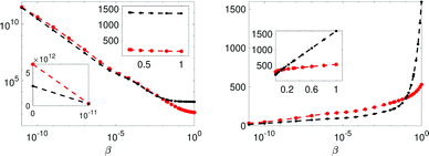 | ||
Fig. 6 The integrand and integral of eqn (12) in the left and right panels respectively, for models Ma (red) and Mb (black). Insets display the linear scale. The error bars are 3 standard errors. The β = 1 value in the left panel is the sought evidence: −2![[thin space (1/6-em)]](https://www.rsc.org/images/entities/char_2009.gif) ln[p(Rexp|Mj,I)]. ln[p(Rexp|Mj,I)]. | ||
With three water-pools of model Mc the lowest χopt2 (at 18) of the four models is reached. The computed evidence is provided in Fig. 7, where although a much better fit is achieved in terms of χopt2, the Bayes-factor dictates very strong evidence against Mc and the three water-pool model (following Jeffrey's scale, see Table 1). This has its origin in the increased Ockham-entropy of model Mc.
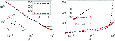 | ||
Fig. 7 The integrand and integral of eqn (12) in the left and right panels respectively, for models Ma (red) and Mc (black). Insets display the linear scale. The error bars are 3 standard errors. The β = 1 value in the left panel is the sought evidence: −2![[thin space (1/6-em)]](https://www.rsc.org/images/entities/char_2009.gif) ln[p(Rexp|Mj,I)]. ln[p(Rexp|Mj,I)]. | ||
Finally, the evidence for alternative two-pool model Md is provided in Fig. 8. Here an interesting observation is that a model with reduced Ockham-entropy (ΔSj,Ockham) is favoured, in spite of its higher χ2(xopt). The boundaries of micelle radius are chosen such that the SED computed correlation time has similar range as in model Ma…Mc. However, noting that the amplitudes are assumed temperature independent makes the physics of the two models slightly different and care is needed not to over interpret the Bayes-factor, noting that a ranking assumes equal probability of the two models compared (see eqn (16)).
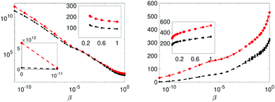 | ||
Fig. 8 The integrand and integral of eqn (12) in the left and right panels respectively, for models Ma (red) and Md (black). Insets display the linear scale. The error bars are 3 standard errors. The β = 1 value in the left panel is the sought evidence: −2![[thin space (1/6-em)]](https://www.rsc.org/images/entities/char_2009.gif) ln[p(Rexp|Mj,I)]. ln[p(Rexp|Mj,I)]. | ||
The approximate model selection criteria listed in Table 6 are the AIC and BIC. By comparing the magnitudes of −2![[thin space (1/6-em)]](https://www.rsc.org/images/entities/char_2009.gif) ln[p(Rexp|Mj,I)] with AIC and BIC it is noted that the smallest AIC value is for Mc thus the wrong order in comparison with the complete integration. The BIC provides qualitatively the same order. Discrepancy is large for BIC compared to −2
ln[p(Rexp|Mj,I)] with AIC and BIC it is noted that the smallest AIC value is for Mc thus the wrong order in comparison with the complete integration. The BIC provides qualitatively the same order. Discrepancy is large for BIC compared to −2![[thin space (1/6-em)]](https://www.rsc.org/images/entities/char_2009.gif) ln[p(Rexp|Mj,I)], larger than a factor two (on log-scale) for Ma and Mc.
ln[p(Rexp|Mj,I)], larger than a factor two (on log-scale) for Ma and Mc.
The Ockham-entropy (see ΔSj,Ockham in Table 6) is lowest for Md and Mb, where the number of parameters is also low. This property reflects the uncertainty in going from prior assumptions of parameters to the final parametrization and can be expected to increase for larger parameter volume.
Clearly we do not know a priori how large MCMC simulations are required, making researchers sometimes stay away from this technique. However, provided is a set of tools to monitor convergence and reproducibility and from a moderate computational investment it is clear how challenging (or easy) problems lie ahead. In particular with the option to follow annealing the experience so far is that MCMC can do well in parametrization of NMR-relaxation, relaxometry and line shape studies,6,7,53,55 and should play an important role in Bayesian evidence calculation.
5.3 Model comparison summary
The components to pay attention to for useful Bayesian model comparison are summarized:• Accurate estimation of experimental variances (see eqn (16)) plays a central role for the outcome model comparison. It is noted that the variance obtained by conventional fit to determine 1/T1 (like Levenberg–Marquardt algoritm), systematically underestimate the variance. To circumvent this, the route5 of calibrating or obtaining estimated variance with multiple experiments is used. An alternative route may be to estimate signal to noise in the measured intensities and apply estimation of 1/T1 and its variance via a separate MCMC run following Fig. 3.
• Parameter prior is here assumed to be uniform, meaning the user sets the min and max of model parameters. The choice of uniform is suitable since parametrisation should be close to that achieved with conventional maximum likelihood methods, to ease the comparison.5,34 Care is needed such that boundaries are set with equivalent strategy, noting that narrow interval around optimal minima may give unfair advantage with ΔSOckham for that model. Also a verification that χ2 is reproducible from multiple starting configurations (Fig. 3) is good to know before going further.
• The Bayesian evidence is accessible via MCMC (see Section 4.2), provided models have relatively low computational cost.
• Note that from a mathematical point of view the Bayesian evidence can be computed for arbitrary models since whole parameter space is integrated. This may allow for instance Lorentzian or non-Lorentzian character of spectral densities to be compared. It is noted, however, that for model comparison we have to assume equal a priori probabilities of the models that may not be true (see eqn (16)). Furthermore, extra attention is required for the motivation of parameter boundaries, not to favour one model more than the other.
6 Conclusions
In this work the methodology of Bayesian model comparison is provided and exemplified with nuclear magnetic relaxation dispersion (NMRD) data. The NMRD profile provides the otherwise difficult to measure slow dynamics in complex materials and biological systems. However, to reach conclusive results requires careful model development to capture the physics and chemistry of the studied system. Thus, Bayesian model comparison fills a gap with quantitative input on how many parameters and mechanisms are reasonable to include in a model based on the data we have. This is a practical question that should always occur when faced with data from a new system.The computational approach follows a thermodynamic integration to compute the Bayesian model evidence from a set of MCMC simulations. The technique followed,41 makes this challenging task feasible. Thus, in addition to quality of fit it is identified that the introduced definition of Ockham-entropy helps us understand the result. To work with entropy is suitable for the physical-chemistry community and valuable in the long-debated explanation of Bayesian evidence.18 Ockham-entropy quantifies the uncertainty in going from prior assumptions, from the limited knowledge before study of the system to the final model parametrization. It is the Ockham-entropy that provides the penalty for over-use of parameters.
It was found that the evidence can be computed with only 10–30 relatively low cost MCMC simulations, in this work each MCMC was completed in 5–20 minutes, meaning that extensive model comparison can be performed with access to a workstation or single cluster-node.
The computed Bayesian evidence rules out the simplicity of one- and the uncertainty of three water-pools in favour of a two-pool model (Ma) based on the current NMRD data. Such a conclusion can not be quantitatively drawn based on a conventional least squares fit (or MCMC parametrization). Furthermore, a two-pool model (Md) involving less uncertainty than (Ma) is provided with improved Bayesian evidence. The proposed model Md suggests a direction for future work on a suitable model that more accurately captures the relevant physics and chemistry. These models can incorporate more experimental data at higher field and another direction is to incorporate information from MD simulations and for instance resolve the order parameter and population.8
It is found that approximate tools to compare models can deviate from the complete integral (AIC), or qualitatively follow (BIC), however, the latter exhibit large discrepancy at logarithmic scale. These findings suggest that MCMC simulation of Bayesian evidence will play an important role in the development of NMRD theory; however, the method is completely general and can find ample use in other areas of physical chemistry as well.
Conflicts of interest
There are no conflicts to declare.Acknowledgements
Prof. Per-Olof Westlund is acknowledged for valuable discussions initiating this work and for sharing NMRD experimental data. The COST Action CA15209 European Network on NMR Relaxometry is acknowledged and prof Pedro Sebastião for pointing out unclear aspects of the first draft. Financial support from the Kvantum institute (University of Oulu, Finland). The computational resources were provided by the CSC – IT Center for Science, Finland and the Finnish Grid and Cloud Infrastructure (FGCI) (urn:nbn:fi:research-infras-2016072533).Notes and references
- R. Kimmich and E. Anoardo, Prog. Nucl. Magn. Reson. Spectrosc., 2004, 44, 257–320 CrossRef CAS.
- J. P. Korb, Prog. Nucl. Magn. Reson. Spectrosc., 2018, 104, 12–55 CrossRef CAS.
- P. J. Sebastião, A. C. Ribeiro, H. T. Nguyen and F. Noack, J. Phys. II, 1995, 5, 1707–1724 CrossRef.
- J. Kowalewski and L. Mäler, Nuclear Spin Relaxation in Liquids: Theory, Experiments, and Applications, Taylor & Francis Group, New York, USA, 2006 Search PubMed.
- P.-O. Westlund, Univers. J. Chem., 2016, 4, 69–73 Search PubMed.
- M. Asadullah Javed, S. Ahola, P. Håkansson, O. Mankinen, M. Kamran Aslam, A. Filippov, F. Ullah Shah, S. Glavatskih, O. N. Antzutkin and V.-V. Telkki, Chem. Commun., 2017, 53, 11056–11059 RSC.
- P. Håkansson, M. A. Javed, S. Komulainen, L. Chen, D. Holden, T. Hasell, A. Cooper, P. Lantto and V. V. Telkki, Phys. Chem. Chem. Phys., 2019, 21, 24373–24382 RSC.
- P. Håkansson, T. Boirin and J. Vaara, Langmuir, 2018, 34, 3755–3766 CrossRef.
- P. Håkansson and P.-O. Westlund, Phys. Chem. Chem. Phys., 2004, 6, 4321–4329 RSC.
- D. Kruk, J. Kowalewski and P.-O. Westlund, J. Chem. Phys., 2004, 121, 2215–2227 CrossRef CAS.
- D. Kruk, P. Rochowski, M. Florek-Wojciechowska, P. José Sebastião, D. J. Lurie and L. M. Broche, J. Magn. Reson., 2020, 106783 CrossRef CAS.
- D. Kruk, A. Herrmann and E. A. Rössler, Prog. Nucl. Magn. Reson. Spectrosc., 2012, 63, 33–64 CrossRef CAS.
- P.-O. Westlund, G. Driver, Y. Wang, T. Sparrman, A. Laaksonen and Y. Huang, Phys. Chem. Chem. Phys., 2017, 19, 4975–4988 RSC.
- K. Åman, P. Håkansson and P.-O. Westlund, Phys. Chem. Chem. Phys., 2005, 7, 1394–1401 RSC.
- P. Håkansson and P. B. Nair, Phys. Chem. Chem. Phys., 2011, 13, 9578–9589 RSC.
- E. Belorizky, P. H. Fries, L. Helm, J. Kowalewski, D. Kruk, R. R. Sharp and P.-O. Westlund, J. Chem. Phys., 2008, 128, 052315 CrossRef.
- W. H. Press, S. A. Teukolsky, W. T. Vetterling and B. P. Flannery, Numerical Recipes in C: The Art of Scientific Computing, Cambridge University Press, New York, 2nd edn, 1992 Search PubMed.
- A. van der Linde, Stat. Neerl., 2012, 66, 253–271 CrossRef.
- R. Hoffmann, V. I. Minkin and B. K. Carpenter, Hyle, 1997, 3, 3–28 Search PubMed.
- I. Solomon, Phys. Rev., 1955, 99, 559–565 CrossRef CAS.
- Y. Ayant, E. Belorizky, J. Alizon and J. Gallice, J. Phys., 1975, 36, 991–1004 CrossRef CAS.
- L.-P. Hwang and J. H. Freed, J. Chem. Phys., 1975, 63, 4017–4025 CrossRef CAS.
- B. Halle, V. P. Denisov and V. Kandadai, Biological Magnetic Resonance, Kluwer Academic/Plenum Publishers, New York, 1999, ch. Structure, vol. 17, pp. 419–484 Search PubMed.
- A. Roch, R. N. Muller and P. Gillis, J. Chem. Phys., 1999, 110, 5403–5411 CrossRef CAS.
- G. Voigt and R. Kimmich, J. Magn. Reson., 1976, 24, 149–154 CAS.
- D. Kruk, A. Kubica, W. Masierak, A. F. Privalov, M. Wojciechowski and W. Medycki, Solid State Nucl. Magn. Reson., 2011, 40, 114–120 CrossRef CAS.
- T. J. Loredo, in Maximum Entropy and Bayesian Methods, ed. P. F. Fougere, Kluwer Academic Publishers, Dordrecht, The Netherlands, 1990, pp. 81–142 Search PubMed.
- R. Trotta, Contemp. Phys., 2008, 49, 71–104 CrossRef CAS.
- J. Rantaharju and J. Vaara, Phys. Rev. A, 2016, 94, 043413 CrossRef.
- P. Honegger, V. Overbeck, A. Strate, A. Appelhagen, M. Sappl, E. Heid, C. Schröder, R. Ludwig and O. Steinhauser, J. Chem. Phys. Lett., 2020, 11, 2165–2170 CrossRef CAS.
- J. P. Korb, P. J. McDonald, L. Monteilhet, A. G. Kalinichev and R. J. Kirkpatrick, Cem. Concr. Res., 2007, 37, 348–350 CrossRef CAS.
- P. Håkansson, L. Persson and P.-O. Westlund, J. Chem. Phys., 2002, 117, 8634–8643 CrossRef.
- V. Wong and D. A. Case, Annual Reports in Computational Chemistry, Elsevier Masson SAS, 2008, vol. 4, pp. 139–154 Search PubMed.
- P. J. Sebastião, Eur. J. Phys., 2014, 35, 1–15 CrossRef.
- R. Andrae, T. Schulze-Hartung and P. Melchior, 2010, arXiv, 1012.3754v, pp. 1–12.
- R. E. Kass and A. E. Raftery, J. Am. Stat. Assoc., 1995, 90, 773–795 CrossRef.
- N. Schenker, J. Am. Stat. Assoc., 1985, 80, 360–361 CrossRef.
- M. A. Newton and A. E. Raftery, J. R. Stat. Soc. B, 1994, 56, 3–48 Search PubMed.
- D. J. C. MacKay, Neural Comput., 1992, 4, 415–447 CrossRef.
- U. von Toussaint, Rev. Mod. Phys., 2011, 83, 943–999 CrossRef.
- W. Von Der Linden, R. Preuss and V. Dose, in Maximum Entropy and Bayesian Methods, ed. R. Fischer, Kluwer Academic Publishers, Dordrecht, 1999, pp. 285–292 Search PubMed.
- B. Halle and H. Wennerström, J. Chem. Phys., 1981, 75, 1928–1943 CrossRef CAS.
- T. Sparrman and P.-O. Westlund, J. Phys. Chem. B, 2001, 105, 12524–12528 CrossRef CAS.
- K. Åman, E. Lindahl, O. Edholm, P. Håkansson and P.-O. Westlund, Biophys. J., 2003, 84, 102–115 CrossRef.
- R. C. Tolman, The Principles of Statistical Mechanics, Dover Publications, New York, 1979 Search PubMed.
- P. Håkansson, BAYES-SELECT (GitHub v1.1), 2020, DOI:10.5281/zenodo.4012179.
- P. Håkansson and M. Mella, J. Chem. Phys., 2008, 129, 124101 CrossRef.
- N. Metropolis, A. W. Rosenbluth, M. N. Rosenbluth, A. H. Teller and E. Teller, J. Chem. Phys., 1953, 21, 1087–1092 CrossRef CAS.
- M. A. Tanner, Tools for statistical inference, Springer-Verlag, New York, 3rd edn, 1996 Search PubMed.
- N. van Kampen, in Stochastic Processes in Physics and Chemistry, ed. N. van Kampen, Elsevier, Amsterdam, The Nederlands, 3rd edn, 2007, ch. 1, pp. 1–29 Search PubMed.
- J. W. Eaton, D. Bateman, S. Hauberg and R. Wehbring, GNU Octave version 5.1.0 manual: a high-level interactive language for numerical computations, 2019, http://www.gnu.org/software/octave/.
- D. Foreman-Mackey, D. W. Hogg, D. Lang and J. Goodman, Publ. Astron. Soc. Pac., 2013, 125, 306–312 CrossRef.
- S. F. Cousin, P. Kadeřávek, N. Bolik-Coulon, Y. Gu, C. Charlier, L. Carlier, L. Bruschweiler-Li, T. Marquardsen, J. M. Tyburn, R. Brüschweiler and F. Ferrage, J. Am. Chem. Soc., 2018, 140, 13456–13465 CrossRef CAS.
- B. Halle, Magn. Reson. Med., 2006, 56, 60–72 CrossRef CAS.
- N. N. Kuzma, P. Håkansson, P. Pourfathi, R. K. Ghosh, H. Kara, S. J. Kadlecek, G. Pileio, M. H. Levitt and R. R. Rizi, J. Magn. Reson., 2013, 234C, 90–94 CrossRef.
Footnote |
| † Electronic supplementary information (ESI) available. See DOI: 10.1039/d0cp04750c |
| This journal is © the Owner Societies 2021 |

