Bayesian inference assessment of protein secondary structure analysis using circular dichroism data – how much structural information is contained in protein circular dichroism spectra?

Abstract

Circular dichroism spectroscopy is an important tool for determining the structural characteristics of biomolecules, particularly the secondary structure of proteins. In this paper we propose a Bayesian model that estimates the covariance structure within a measured spectrum and quantifies the uncertainty associated with the inferred secondary structures and characteristic spectra associated with each secondary structure type. Furthermore, we used tools from Bayesian model selection to determine the best secondary structure classification scheme and illustrate a technique for comparing whether or not two or more measured protein spectra share the same secondary structure. Our findings suggest that it is not possible to identify more than 3 distinct secondary structure classes from CD spectra above 175 nm. The inclusion of data from wavelengths between 175 and 200 nm did not substantially affect the ability to determine secondary structure fractions.

---

Introduction

Proteins are the main focus of a wide range of areas of research, from biochemistry to cellular biology to drug discovery. Since a protein's structure determines its functionality, many spectroscopic techniques have been developed, each one designed to explore an aspect of these biomolecules.¹ Far ultra-violet (<260 nm) circular dichroism (CD) spectroscopy is an important and successful spectroscopic technique that gives meaningful information about the secondary structure of proteins,^2–6i.e. its local shape. CD is particularly useful when only samples in solution are available and techniques such as X-ray crystallography cannot be used. Thanks to the fast and cheap nature of the experiments, CD is an ideal tool for testing controls in many protein screening assays related to the drug discovery process.⁷

In recent years large datasets of CD spectra have been produced^8–10 which enable the relationships between secondary structure and CD data to be explored through mathematical modeling and statistical analysis. In CD spectroscopy the main approach to find the secondary structure has been to deconvolute a spectrum into a weighted sum of so-called characteristic spectra by a variety of different algorthims.^11–14 For a given protein the relative weight of each characteristic spectrum enables calculation of the abundance of the respective structure element from known data about the structure of the proteins making up the reference set. From a statistical perspective these approaches share the same model structure: a linear model, and use standard regression techniques to fit the model. There are a few exceptions, such as neural network model approaches,^15–17 though the self-organising map neural network approaches also involve finding a best match combination of spectra and assigning secondary structures from them. The implicit assumption behind a linear model is that the errors at each wavelength are uncorrelated and have equal variance, even though evidence for a more complicated error structure has been recently pointed out,¹⁸ with variance depending on the wavelength. There are also significant amounts of correlation within some parts of the spectrum. In this work we used a Bayesian approach in which we keep the linear structure but let the covariance matrix of the CD spectra be as general as possible in order to identify crucial dependencies within the CD spectra and weight the information in the most coherent way. Firstly, our approach can be used as a secondary structure estimation method or to enhance existing algorithms. Secondly, we can use tools from Bayesian model selection to investigate the secondary structure classifications schemes that can be determined successfully from CD data. In particular, we consider which secondary structures can be assigned from CD data between 175–260 nm. We also explore possible uses of the posterior uncertainty.

Methods

Notation

Let c_x be the CD spectrum measured from an individual protein x, formally a row with n_λ entries along the wavelength range, in our case usually for data measured between 175 nm and 260 nm with steps of 1 nm. The CD spectrum units are the per residue molar absorption units Δε measured in mol⁻¹ dm⁻³ cm⁻¹. Let  f_x represent the secondary structure fractions, a row vector of n_s secondary structure elements that must sum to one. Finally let B be a matrix of dimension n_s × n_λ, whose rows hold the characteristic CD spectra for each secondary structure class. The common hypothesis in the linear model is:

c_x = f_xB + w_x (1)

where the row vector w_x represents the error between the predicted spectrum and the observed data. Even though eqn (1) seems a typical regression problem it has challenging features to be faced. First, eqn (1) is actually a special kind of inverse problem¹⁹ where both the parameters f_x and the design matrix are unknown. To overcome this lack of knowledge about the design matrix it is common practice to use a reference set, a dataset of proteins with known secondary structure and CD spectra, to estimate B. The secondary structure fractions f_x for proteins in a test set can then be determined. Many existing algorithms do not use the full information from the reference set but often have a variable selection step¹³ from which to identify a subset of proteins closely related to the test protein x to estimate the matrix B. Second, the elements of f_x are not independent but are constrained to sum to one and usually constrained to be non-negative numbers, as they represent the proportion of the molecule that belongs to each secondary structure class:

0 ≤ f_i ≤ 1, for i = 1,…,n_s (2)

Each existing approach has a different method for satisfying such constraints, sometimes based on ad hoc criteria and leading to an approximate solution, e.g. the sum can be in the region 1 ± 0.05.¹¹

A third challenge relates to the common assumptions of considering normal and independent variables for the error w_x. If Σ is the covariance matrix within a spectrum, then it is usually chosen to be a diagonal matrix, not taking into account possible correlations that a spectrum is known to display.

In the following sections we discuss a Bayesian approach to inference where the fraction vector f_x and characteristic matrix B are estimated jointly, making full use of the information in the reference set, i.e. without variable selection. We introduce a Dirichlet prior for the fractions f_x to capture the constraints (2) and (3) and most importantly we estimate a general covariance matrix Σ for the errors, allowing the model to learn the correct covariance structure from the reference set.

Model and likelihood

In order to use all the data in a reference set to estimate secondary structures of unknown proteins, we proceed as follows. Let C be the matrix denoting all the spectroscopic data, whose first n_r rows are the CD spectra of the reference set, and the remaining n_t are the spectra of the proteins in the test set to be analyzed, each row having length n_λ. In the same way let F be the (n_r + n_t) × n_s matrix of secondary structure fractions for all the proteins, where n_s is the number of secondary structure classes. We treat all of the proteins the same, whether they are in the reference set or not, and any unknown secondary structure fractions are treated as parameters and inferred. The matrix formulation of the model for the CD spectra is:

C = FB + W (4)

where the n_s rows of B can be thought of as the characteristic CD spectra for each secondary structure class and W is the random matrix representing experimental variability and any other disagreement between the observed data and predicted spectra, such as lack-of-fit.

We suppose that the CD spectra are normally distributed about BF with the same general covariance matrix Σ, which will be inferred from the data. Furthermore, we assume no dependence between the spectra of different proteins. This leads to the error W taking the form of a matrix normal distribution:

where is the (n_r + n_t) × n_λ zero matrix, I_nr+nt is the (n_r + n_t) × (n_r + n_t) identity matrix. The matrix Σ captures the covariance structure along the rows of W (among the wavelengths in a spectrum), whilst the columns of W (representing the proteins) are assumed to be independent. Thus, the likelihood function is the matrix normal density:where F_t is the submatrix of unknown secondary structure fractions related to the n_t proteins in the test-set.

Prior distributions

The model parameters are the set {F_t,B,Σ}, and prior knowledge is factorized as follows:

π(F_t,B,Σ) = π(F_t)π(Σ)π(B|Σ,F_t)

The conditional dependence structure of the model is shown in the ESI (Fig. S1†). For every protein in the test set we chose independent Dirichlet-distributed priors:

f_x ∼ Dir(α), for x = n_r + 1,…,n_r + n_t

and in applications we used the Jeffreys prior

α = [1/2,…,1/2]_ns

The Dirichlet distribution is a natural choice because the parameter space is a n_s-dimensional simplex defined by the constraints (2) and (3).

For B and Σ we follow the common choice for Bayesian linear models and choose conjugate priors.²⁰ The prior for B is the matrix normal distribution with mean M and covariance matrices U and Σ. In applications the matrix M was chosen to be the zero matrix, which is symmetrical with respect to positive and negative signals – reflecting left and right-handed chirality – and has a shrinkage effect. The matrix U represents the covariance between the secondary structure classes and a g-prior²¹ is chosen to account for possible relationships within the secondary structures:

U = g(F^TF)⁻¹.

Following George and Foster,²² we set the hyper-parameter g = n_r, the dimension of the reference set, this choice is referred to as the unit information prior.

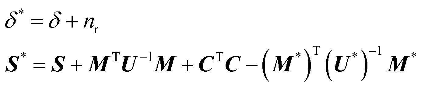
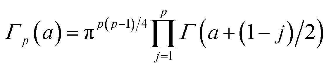
The prior for the n_λ × n_λ covariance matrix Σ, representing the covariance structure within a CD spectrum, is the inverse-Wishart distribution. The inverse-Wishart W_n⁻¹(δ,S) is the generalization of the inverse-Gamma distribution in n-dimensions, having density:

for positive definite Σ where
and Γ[·] is the Euler Gamma function.

In applications we chose δ = n_λ, representing the degrees of freedom, and S = I_nλ, a covariance matrix with no correlation and unit variances. In summary, we can write for the priors:

McMC algorithm

The computation of the posterior distribution π(F_t,B,Σ|C) is done using Markov chain Monte Carlo (McMC). Due to the conjugate prior specified in eqn (7), the full conditional distribution for B follows a matrix normal distribution,^20,23with updated parameters:

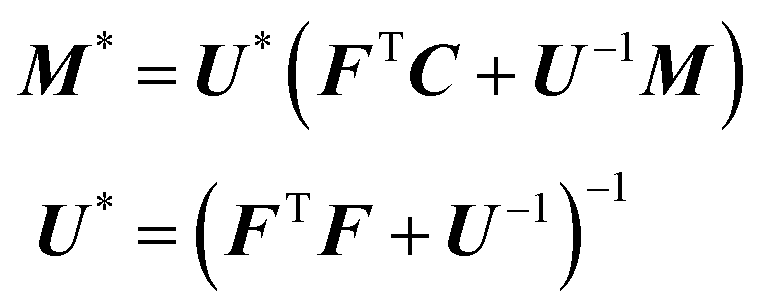
The full conditional distribution for the covariance matrix Σ is given by,

Σ|(C,F_t) = W⁻¹(δ*,S*) (10)

with

The conjugate priors for B and Σ allow us to integrate out these parameters and obtain a closed-form expression for the likelihood:

where is the multivariate gamma function. Integrating out these parameters greatly improves the mixing of the resulting MCMC algorithm.

The prior for F_t is not conjugate and so these parameters are updated using a Metropolis–Hastings step, for each protein individually. Proposals are generated using an adaptive Dirichlet random walk algorithm. If f_x is the row within F_t for protein x, then the proposal is

where the scaling factor β_x is increased by 0.234 × 10/i on iteration i if the proposal is rejected and decreased by 0.776 × 10/i if the proposal is accepted. This adapts each proposal to target an acceptance rate of 0.234. If samples for Σ and B are required then these can be drawn from eqn (9) and (10) respectively given the samples from F_t.

Protein data and reference sets

Open access CD datasets are available in the Protein Circular Dichroism Data Base (PCDDB)⁹ with high quality data obtained using Synchrotron Radiation Circular Dichroism. From the PCDDB we took the SP175 dataset⁸ containing spectra for 71 globular proteins. We considered three secondary structure classification schemes. The first comes from the DSSP algorithm^24,25 which includes 8 classes: α-helix, 3-10-helix, β-strand, turn, bend, π-helix, β-bridge, irregular. In the SP175 database there is almost no contribution from π-helix, so in all analyses we combined this class with irregular, leaving 7 classes in total. The second scheme we considered included just 3 classes taken from DSSP: α-helix, β-strand and other (referred to as DSSP_red), comprising the sum of the remaining categories. The third scheme was defined through the CD scheme²⁶ and following.²⁷ We refer to this as the SELCON scheme whose six secondary structure classes are: regular helix (the middle of any helix), distorted helix (the two residues on each end of a helix), regular β-strand, distorted β-strand (1 residue on the end of each strand), turn and other. Finally, we also consider the BeStSel classification scheme from ref. 27. Their eight classes are regular α-helix, distorted α-helix, left-twisted β-strand, relaxed β-strand, right-twisted β-strand, parallel-strand, turn and other. For details of the interrelationship between these classification schemes, see ref. 27.

Performance indices and cross validation

Algorithms are usually tested with leave-one-out cross validation. In this methodology one protein at a time is removed from the reference set and is specified to be the test set. Repeating this for each protein in the original reference set gives n_r estimated vectors of secondary structure, which we will refer to as the cross-validation set.

The performance of an algorithm, i.e. comparing a secondary structure estimate with the X-ray experiment value, taken as “truth”, is performed with two measures commonly accepted in the CD literature: the root-mean-square deviation (RMSD) δ and the Pearson correlation coefficient r. They are defined for a protein x with true value as

where f̄ denotes the mean of the entries in the vector f and σ_f denotes the standard deviation. These two quantities are related to single protein estimation only. In order to measure the performance of the algorithm, averages over the cross-validation set are taken. In particular the average RMSD, has been used by other authors, see for example,¹¹ as prediction error of any (future) protein structure estimates.

As well as measuring global performance, it is interesting to know how the algorithm behaves for each secondary structure class. The RMSD δ_i and correlation coefficient r_i, for class i, are calculated similarly to (12) and (13), but performing the sum over the proteins x in the cross-validation set. The measures are known in the literature as performance indices of the analysis and used for comparisons between methods. A variety of more sophisticated performance measures also exist, which attempt to normalise by the amount of variation inherent within each class. One such measure is ζ_i = σ_i/δ_i,²⁸ where σ_i is the standard deviation of the secondary structure fractions for class i. If ζ_i is greater than 1 then the average error is less than a random choice from the reference set.

Our Bayesian approach produces a posterior distribution over secondary structures rather than a single estimated secondary structure vector. Unless otherwise stated we have used the posterior mean secondary structure as the estimated structure.

Model comparison via marginal likelihoods

An advantage of our Bayesian approach is that it becomes possible to use Bayesian model comparison to answer questions of scientific interest, such as which secondary structure classes can be identified from the reference proteins and whether two CD spectra share the same secondary structure. In order to choose between models {M_i : i ∈ I}, we examine the posterior probability in favour of model M_i, given by:where π(C|M_i) is the marginal likelihood for model i.

There is no closed form available for the marginal likelihoods for these models. However, due to the conjugate priors for B and Σ, we can integrate out these two parameters to obtain an expression for π(C|F_t), see eqn (11).

To obtain an estimate of the full marginal likelihood

π(C) = ∫ π(C|F_t)π(F_t) dF_t

we apply methodology that uses samples from the McMC to inform an importance sampling estimator for the marginal likelihood.^29,30 First samples are obtained from the marginal posterior π(F_t|C) using the usual McMC algorithm. Secondly a parametric distribution (with known normalising constant) is fitted to the McMC samples, usually a multivariate normal distribution. Let q(F_t) denote the density of this distribution. In this application only the first (n_s − 1) components of each secondary structure vector are used, as the final component can be recovered from constraint (3). Thirdly, N samples (labelled F_t⁽¹⁾,…,F_t^(N)) are drawn from q(F_t). Finally, we obtain the importance sampling estimator for the marginal likelihood for a specific model M_i:

It is desirable to make q(F_t) over-dispersed relative to the true posterior, to make the variance of the importance sampling estimator as small as possible. This can easily be achieved by replacing q(.) with a multivariate t-distribution or a mixture of the multivariate normal and the prior π(F_t). For full details of this methodology see Touloupou et al.²⁹

Results and discussion

Secondary structure estimation

There is significant debate in the literature as to whether CD spectra from 260–175 nm contain enough information to give different spectral signatures for any folds more than α-helix and β-sheet. So, to avoid trying to answer multiple questions simultaneously we chose to assess the accuracy of secondary structure estimation using our Bayesian approach by performing a leave-one-out cross validation over the reference set SP175 with the simplest classification scheme, DSSP_red. In Table 1 we have compared our model predictions with some of the other algorithms, including SELMAT3,^8,26 Partial Least Squares (PLS), Principal Component Regression (PCR), Neural Network (NN), and Support Vector Machines (SVM) using results taken from ref. 31. Broadly speaking, our Bayesian approach is competitive with the other approaches for α-helix, but does not do as well for β-sheet. Results for the normalised measure ζ are given in the ESI (Tables S1 and S2†). Overall, there is no clear best approach.

Table 1 Cross-validation results for the SP175 proteins with 3 secondary structure classes from DSSP: α-helix, β-sheet and other structure. Results for competing approaches (SELMAT3, PCR, PLS, NN and SVM, taken from ref. 31) are shown. The best performing approach for each measure is given in bold. δ is RMSD and r is the correlation

Method	α-helix		β-sheet		Other
	δ	r	δ	r	δ	r
Bayesian	0.061	0.96	0.127	0.77	0.137	0.65
SELMAT3	0.063	0.96	0.083	0.86	0.078	0.70
PCR	0.057	0.97	0.069	0.91	0.066	0.80
PLS	0.053	0.97	0.073	0.90	0.068	0.78
NN	0.055	0.97	0.067	0.91	0.062	0.82
SVM	0.057	0.97	0.069	0.91	0.066	0.79

---

Table 2 (which is rotated with respect to Table 1) shows the leave-one-out cross validation results using the SELCON secondary structure scheme, over the SP175 reference set. This time the Bayesian approach does not perform well, particularly for the classes turn and other. Results for the normalised measure ζ are given in the ESI,† where a value above one indicates an improvement above choosing at random from the reference set. For both SELMAT3 and PLS the value of ζ is just 1.04 for turn. The results of Table 2 and the normalised measure ζ in the ESI† indicate that there is not enough information, even in spectra down to 175 nm to differentiate the 6 SELCON secondary structure motifs.

Table 2 Cross-validation results for the SP175 proteins with the SELCON secondary structure scheme. Results for competing approaches SELMAT3 and PCR are taken from ref. 31. The best performing approach for each measure is given in bold

Structure	Bayesian		SELMAT3		PLS
	δ	r	δ	r	δ	r
Regular helix	0.090	0.836	0.048	0.956	0.040	0.971
Distorted helix	0.129	0.043	0.035	0.809	0.036	0.791
Regular β-strand	0.090	0.695	0.073	0.792	0.063	0.853
Distorted β-strand	0.281	−0.081	0.020	0.913	0.023	0.889
Turn	0.201	0.098	0.052	0.325	0.052	0.332
Other	0.169	0.278	0.050	0.717	0.050	0.720

---

We hypothesise that the underlying cause of this is that in our Bayesian approach we do not perform variable selection to identify a subset of the reference set for each cross-validation step. Variable selection has been found to avoid inconsistencies between CD spectra and secondary structure schema to improve the quality of the analysis.^13,27 We have chosen not to select a subset of proteins for the reference set that are similar to the test protein as we wanted to use all the information from the reference set. If an α-helix, for example, has a characteristic signal then it should be consistently present in spectra for all proteins containing α-helice. We do believe that other protein features, such as distortions at the ends/joins, side chains and higher order structures, can obscure or modify this signal. These features are not necessarily represented in any of the secondary structure characterisation schemes. Bayesian analyses usually consider information from the whole data set and use the parameter uncertainty to weight the information content rather than discarding information that does not fit the pattern.

Another consideration is that early, landmark papers that found a need for variable selection^32,33 were using techniques such as partial least squares (PLS) to identify the basis vectors from a comparatively small number of reference proteins. Whilst PLS will always succeed in producing n basis vectors from n (linearly independent) protein measurements, it is not clear from this kind of analysis how many of the resulting vectors contain only contributions from the underlying signal. The variability inherent in the dataset will certainly dominate in the last basis vectors and (hopefully) the signal will dominate in the first few vectors, but it may be the case, especially when the number of proteins in the reference set is small, that the basis vectors in the middle are actually representing the variability in the dataset as much as clearly identified secondary structures. The immediate conclusion that could be made is that variable selection is important for making predictions using existing classification schemes. However, the apparent success of the variable selection approaches depends on having ‘like’ proteins in the reference set which is simply not always possible with unknown proteins.

Identifiability of secondary structure classes

To explore what can be identified from the CD spectra, we used the model selection methodology to determine which secondary structure classes can be identified from the amount of information in a given reference set. We used the 3 classification schemes: DSSP, SELCON and BeStSel, and we also defined simpler schemes from within these by summing together components. Since DSSP, SELCON and BeStSel have 7, 6 and 8 secondary structure classes respectively, we considered 5220 schemes in total.

Each potential secondary structure scheme is represented by a different design matrix of secondary structure fractions F. Given F, we can evaluate the marginal likelihood for the model analytically from eqn (11) since the test set is empty here. These marginal likelihoods can be used to produce Bayes factors comparing any pair of models and, once prior probabilities for each model have been specified, the posterior probability in favour of each secondary structure scheme can be identified. Following Scott et al. and Spencer et al.^34,35 we adjusted for multiplicity caused by different numbers of structures in the different models by first assigning a prior distribution over the number of classes, and then dividing the mass equally amongst the models that have the same number of classes. In applications we chose a uniform prior over the number of classes between 3 and the maximum as summarised in Table 3.

Table 3 Models with posterior probability greater than 0.001 within each classification scheme and in a comparison between all schemes combined

Classification schemes	Posterior probability	Log marginal likelihood	Secondary structure classes
DSSP	0.510	−7296.235	α-helix	310-helix+β-strand + bend	β-bridge + turn + other
	0.448	−7296.366	α-helix	β-strand + bend	310-helix+β-bridge + turn + other
	0.028	−7299.131	α-helix+β-bridge	β-strand + bend	310-helix + turn + other
	0.013	−7299.892	α-helix+β-bridge	310-helix + β-strand + bend	Turn + other
SELCON	0.999	−7319.677	Regular α-helix	Regular β-strand	Distorted α-helix + distorted β-strand + turn + unordered
BeStSel	1.000	−7205.936	Regular α-helix	Left β-strand + relaxed β-strand + parallel	Distorted α-helix + right β-strand + turn
DSSP, SELCON, BeStSel	1.000	−7205.936	Regular α-helix	Left β-strand + relaxed β-strand + parallel	Distorted α-helix + right β-strand + turn

---

We performed model comparison to find the most appropriate model within the three secondary structure schemes individually and also amongst all three schemes. Again, to avoid bias towards schemes with larger numbers of models, we first assigned a prior probability of one third to each scheme and then divided this prior mass amongst the models stemming from each scheme as before. Table 3 gives all the schemes with posterior probability greater than 0.001. For DSSP the posterior probability is largely split between 2 very similar models that differ only in where 3–10 helix is included. For the SELCON scheme the best model included regular helix and regular β-strand as separate components and combined the remaining classes together. The best model for the BeStSel scheme included 3 basis spectra: regular α-helix; the sum of left-β-strand + relaxed and β-strand + parallel, and the remaining components. This model had by far the largest marginal likelihood and therefore it also dominates the comparison between the 3 classification schemes. Interestingly under all three classification schemes just 3 basis spectra were needed to explain the data. These all included a single α-helix class in the best model and combined class including β-strand as the second basis spectrum. It may be concluded that no more than three distinct structures that can be assigned from the data between 175–260 nm.

To investigate this further we performed a cross-validation with the BeStSel secondary structure scheme with the highest marginal likelihood for 3, 4 and 5 secondary structure classes. Results for the normalised measure ζ are given in ESI.† We repeated each analysis using data down to 175, 180, 185, 190, 195 and 200 nm. The results show that for all these ranges our approach can successfully identify 3 secondary structure classes, as the ζ values are all substantially above 1. This provides at least some evidence that our model selection approach, which favours the BeStSel secondary structure scheme, does so with good reason. The ζ values decay slightly as the lowest 5 nm of the spectra are sequentially removed, but not substantially. However, when we try to infer more than 3 secondary structure classes then there is always at least one class that has a ζ value below one.

These results are an interesting contrast with the accepted literature consensus e.g.³⁶ which is that data to 200 nm contain two independent pieces of information (which with the requirement of the sum of components adding to 1 makes three pieces of information), data to 190 nm contain 3–4, and data to 178 nm provide 5. The origin of this consensus is in a single value decomposition approach based on 16 reference spectra performed in 1985 by Manavalan and Johnson.³³ Our work indicates that although CD spectra to lower wavelengths do contain more information about protein structure, it cannot be translated into increasing numbers of traditional well-defined structures.

Spectra covariance matrix and spectral quality

As shown in Fig. 1, α-helix and β-sheet content are in practice fairly anti-correlated, whereas turns and bends scatter about a mean value largely independent of helix and sheet content until high helix content where bonded turns decrease. So, we wished to characterise the covariance structure of a CD spectrum. We used the SP175 reference set to calculate the posterior distributions of the transformation matrix B and covariance matrix Σ using the DSSP_red scheme (α-helix, β-sheet and other). In this case the test set is empty and so there is no need for McMC – samples from the posterior can be drawn directly from eqn (9) and (10).

Fig. 1 Plots of fraction (out of a total of 1) of secondary structure motifs versus α-helical content for the proteins in reference set SP175 using the DSSP structure annotation.

Fig. 2(a) shows the three characteristic spectra that were estimated from the SP175 reference set: the thick lines are the posterior median of the three columns of B and the shaded area captures a 95% credible interval. In Fig. 2(b) we show an image representation of the posterior mode for Σ, given by S*/(n_r + n_λ + 1). Thus, we conclude that despite the tendency for α-helix and β-sheet to act like a see-saw (Fig. 1), they have distinct typical shapes that combine to give an observed spectrum.

Fig. 2 (a) Plot of the estimated characteristic spectra for α-helix, β-sheet and other structure based on an analysis of the SP175 reference set. The lines represent the posterior median and the shaded areas represent 95% credible intervals for the characteristic spectra. (b) The posterior mode for the covariance matrix within a CD spectrum Σ, based on the same analysis.

Fig. 2(a) and (b) show that there is more uncertainty/variability for lower wavelengths and relatively little variability above 250 nm where the spectra approach zero. The wide diagonal green band in Fig. 2(b) indicates a strong correlation between errors at similar wavelengths. Conversely the red patches indicate a negative correlation between very low wavelengths and the middle of the spectrum, indicating that if the observed spectrum is lower than predicted at around 190 nm, for example, then it will be higher than expected in the 210–230 nm region.

A key feature of our modelling approach is that we estimate covariance structure of a CD spectrum directly from the data, allowing the measurement uncertainty to change with wavelength and errors at similar wavelengths to be correlated. Most existing algorithms implicitly assume that the errors are uncorrelated so that Σ is forced to be a diagonal matrix.^11–14,27 This forces errors at similar wavelengths to be uncorrelated, when in reality we expect them to be similar. Fig. 2(b) shows the estimated error structure of a spectrum and strong correlation structure is clearly present. Furthermore, the diagonal elements, representing variances, have a strong dependence on the wavelength, with larger variances at lower wavelengths. This feature is expected due to how the CD instrument works. At shorter wavelengths the high-tension voltage of the photomultiplier tube, which transforms the light signal into an electrical signal, is increased to compensate for the lower power of the light source. Thus, an increased variability in the low UV region data (λ < 200 nm) is a known feature of this kind of spectrum, but gives a worrying indication that the reference spectra are not as perfect as one might hope in the low wavelength region. Above 200 nm the covariance gradually fades to zero along the diagonal indicating higher quality data in this region.

Fig. 2(b) also shows that close wavelengths are positively correlated but further wavelengths are negatively correlated. Two potential mechanisms for generating a negative correlation structure are shown in Fig. 3. Negative correlation could be due to differences in the spectra of proteins in the reference set with similar overall secondary structure content. For example, if two proteins, with close secondary structure, display two similar spectra with a small scaling factor (concentration error) or a slight translation on the wavelength axis (poor wavelength calibration),³⁷ these differences would lead to a fitted spectrum somewhere in between and the residual would be positive correlated in the short distance but negative for further wavelengths as the spectra change sign or gradient. Another source of disagreement between the observed and fitted spectra could be a lack of fit of the model, which might stem from the different between, n helical residues being in 5 small helices or 1 large one.²⁷ Nevertheless, our methodology is able to identify these features of the CD data covariance structure, allowing it to properly weight the information when performing secondary structure estimation or spectral comparison.

Fig. 3 Schematic representation of two kinds of error that lead to the correlation structure observed in Fig. 2(b). In (a) a translation to the left of 2 nm and (b) a rescaling of the spectrum by a factor of 0.7 (dash line) was applied to the true spectrum (solid line). The true spectrum was bovine gamma-E protein (PDB entry 1m8u). The bottom row plots show the difference between the true spectrum and the spectrum with error.

Do two proteins with similar spectra have the same secondary structure?

The second model selection question we address is to determine whether two or more similar looking protein CD spectra correspond to proteins with the same secondary structure or not. Let c_x and c_y be the spectra from two protein samples x and y. Let M₀ be the model assuming the two proteins have the same secondary structure. Let M₁ be the alternative model in which we look for two separate secondary structures for x and y. Schematically we have:

Using eqn (14) and (15) we evaluate the marginal likelihood and the posterior model probability for the two models. As a model prior we chose P(M_i) = 1/2 for i ∈ {0,1}.

Under model M₀ the spectra c_x and c_y are assumed to have the same secondary structure f : f_x = f_y. Here F_t has two identical columns, both equal to f. Under model M₁ we obtain posterior samples for f_x and f_y, which represent the two columns of F_t. For both models the marginal likelihood can be estimated with the importance sampling estimator (15). However, for model M₀ the importance proposal must be fitted to posterior samples from just one column of F_t, and the second column is set equal to the first; whilst in M₁ the two columns are sampled independently.

We tested the comparison method for two CD spectra with two simulated examples. For our first spectrum c_x, we take the spectrum of sucrose porin protein (scrY, PDBID: 1a0s) from the MP180 dataset.³⁸ To obtain our second spectrum c_y, we added noise to c_x. First, we added white noise (Fig. 4 left column), with standard deviation equal to 0.12Δε. Second, Fig. 4 right column, we added multivariate Gaussian noise with zero mean and covariance matrix given by the posterior mode for Σ, representing the usual experimental variability. For both comparisons we fitted the competing models using 1000 iterations of the MCMC and then used 100 000 importance samples drawn from a t-distribution with 3 degrees of freedom. The model comparison with white noise suggests that the secondary structures are different (posterior probability of a difference 0.987). For the experimental noise, the model comparison favours the simpler model, that the two secondary structures are the same (posterior probability of a difference 0.033). Although the magnitude of the white noise is much smaller than the experimental variability (see Fig. 4 lower plots), the model comparison exercise has correctly identified that the white noise does not conform to experimental variability.

Fig. 4 Top row: plots of the scrY spectrum (black) and the scrY spectrum with added noise (red). Bottom row: plots of the difference between the two spectra. Left column: Gaussian white noise, right column: multivariate Gaussian noise with covariance structure representing usual experimental variability (see text for details).

Conclusions

In this paper we first validated our Bayesian approach for CD structure fitting, then we used the model selection methodology to compare secondary structure classification schemes. We found that the BeStSel scheme was better at explaining the SP175 reference set than the competing schemes. We also found that the preferred model included just 3 basis spectra, which suggests that attempting to predict more than 3 types of structure will lead to much greater uncertainty in the estimation. By looking at the normalised measure ζ we showed that CD data between 175–260 nm contain only enough information to assign 3 secondary structure motifs (some version of α-helix and β-strand, and the rest). In contrast to the general consensus, our work indicates that although CD spectra to lower wavelengths do contain more information about protein structure, it cannot be translated into increasing numbers of traditional well-defined structures that can be determined. We would advise using data down to at least 195 nm, with lower cut-offs slightly improving the structure fitting. In practice more structures can be assigned if the reference set is reduced to include only spectra similar to the unknown protein.

We have showed the importance of capturing the correct covariance structure within a spectrum. Our Bayesian approach accounts carefully for the uncertainty in measurement as well as the unknown basis spectra. Three basis spectra and their uncertainty envelopes were generated. The experimental uncertainty could be removed by replacing the smoothed averaged reference and test spectra in our calculations with multiple individual repeats, preferably from different experiments and instruments. The result would be the spectral/structural variation for a revised Fig. 1(a). With replicate spectra the model could be further developed by adding a multivariate random effect associated with each protein, so that it would become possible to quantify the variation due to measurement error and poor model fit separately.

Whether our Bayesian method identifies two spectra as different depends strongly on the kind of noise in the two spectra and we were able to distinguish between a typical CD error, inferred from the reference set, and another kind of noise, i.e. a Gaussian random error. This comparison method has potential wide applications, as a suitable tool to monitor structural changes in protein screening assays, production processes or drug discovery processes.

A second direction for future development would be to combine data from different techniques such as linear dichroism, infrared absorbance spectroscopy, Raman, NMR etc.^3,39–46 that might provide orthogonal information about protein structure. By fully characterising the measurement uncertainty with each technique, our Bayesian approach provides a natural way to combine and to correctly weight information across techniques, unlike existing approaches^28,47 in which the influence of each technique depends only on the relative numbers of points observed in each spectrum.

Conflicts of interest

There are no conflicts to declare.

Acknowledgements

Jacopo Franco's contributions to the early stages of this project are gratefully acknowledged, however he is unaware that this paper is being submitted for publication as we have no contact details for him. Therefore, he does not take any responsibility for the contents. JF is grateful for funding from the Centre for Analytical Science Marie Curie Innovative Doctoral Programme, funded by the EU, whilst at the University of Warwick.

References

1. J. T. Pelton and L. R. McLean, Anal. Biochem., 2000, 277, 167–176.
2. S. M. Kelly, T. J. Jess and N. C. Price, Biochim. Biophys. Acta, 2005, 1751, 119–139.
3. B. Nordén, A. Rodger and T. R. Dafforn, Linear dichroism and circular dichroism: a textbook on polarized spectroscopy, Royal Society of Chemistry, Cambridge, 2010.
4. R. W. Woody, in Circular dichroism principles and applications, ed. K. Nakanishi, N. Berova and R. W. Woody, VCH, New York, 1994.
5. N. Sreerama and R. W. Woody, Anal. Biochem., 1993, 209, 32–44.
6. W. J. Johnson, Annu. Rev. Biophys. Biophys. Chem., 1988, 17, 145–166.
7. C. Bertucci, M. Pistolozzi and A. De Simone, Anal. Bioanal. Chem., 2010, 398, 155–166.
8. J. G. Lees, A. J. Miles, F. Wien and B. A. Wallace, Bioinformatics, 2006, 22, 1955–1962.
9. L. Whitmore, B. Woollett, A. J. Miles, D. Klose, R. W. Janes and B. A. Wallace, Nucleic Acids Res., 2011, 39, D480–D486.
10. K. A. Oberg, J.-M. Ruysschaert and E. Goormaghtigh, Protein Sci., 2003, 12, 2015–2031.
11. N. Sreerama and R. W. Woody, Anal. Biochem., 2000, 287, 252–260.
12. L. A. Compton and W. C. Johnson, Anal. Biochem., 1986, 155, 155–167.
13. P. Manavalan and C. W. Johnson, Anal. Biochem., 1987, 167, 76–85.
14. I. H. van Stokkum, H. J. Spoelder, M. Bloemendal, R. van Grondelle and F. C. Groen, Anal. Biochem., 1990, 191, 110–118.
15. M. A. Andrade, P. Chacon, J. J. Merelo and F. Moran, Protein Eng., 1993, 6, 383–390.
16. V. Hall, A. Nash, E. Hines and A. Rodger, J. Comput. Chem., 2013, 34, 2774–2786.
17. V. Hall, M. Sklepari and A. Rodger, Chirality, 2014, 26, 471–482.
18. N. P. Chmel, P. Scott and A. Rodger, Chirality, 2012, 24, 699–705.
19. R. C. Aster, B. Borchers and C. H. Thurber, Parameter estimation and inverse problems, Academic Press, 2011.
20. P. J. Brown, M. Vannucci and T. Fearn, J. Roy. Stat. Soc. B Stat. Methodol., 1998, 60, 627–641.
21. A. Zellner, Bayesian inference and decision techniques: Essays in honor of Bruno De Finetti, 1986, vol. 6, pp. 233–243.
22. E. George and D. P. Foster, Biometrika, 2000, 87, 731–747.
23. D. G. T. Denison, Bayesian methods for nonlinear classification and regression, Wiley, Chichester, 2002.
24. R. P. Joosten, T. A. Te Beek, E. Krieger, M. L. Hekkelman, R. W. Hooft, R. Schneider, C. Sander and G. Vriend, Nucleic Acids Res., 2011, 39, D411–D419.
25. W. Kabsch and C. Sander, Biopolymers, 1983, 22, 2577–2637.
26. N. Sreerama, S. Y. Venyaminov and R. W. Woody, Protein Sci., 1999, 8, 370–380.
27. A. Micsonai, F. Wien, L. Kernya, Y.-H. Lee, Y. Goto, M. Refregiers and J. Kardos, Proc. Natl. Acad. Sci. U. S. A., 2015, 112, E3095–E3103.
28. K. A. Oberg, J.-M. Ruysschaert and E. Goormaghtigh, Eur. J. Biochem., 2004, 271, 2937–2948.
29. P. Touloupou, N. Alzahrani, P. Neal, S. E. Spencer and T. J. McKinley, Bayesian Analysis, 2019, 1–32.
30. M. Clyde, J. Berger, F. Bullard, E. Ford, W. Jfferys, R. Luo, R. Paulo and T. Loredo, Statistical Challenges in Modern Astronomy IV, 2007, vol. 371, p. 224.
31. J. G. Lees, A. J. Miles, R. W. Janes and B. A. Wallace, BMC Bioinf., 2006, 7, 507.
32. J. P. Hennessey and W. C. Johnson, Biochemistry, 1981, 1085–1094.
33. P. Manavalan and W. C. Johnson, Proc. Int. Symp. Biomol. Struct. Interactions, Suppl. J. Biosci., 1985, 8, 141–149.
34. J. G. Scott and J. O. Berger, Ann. Stat., 2010, 38, 2587–2619.
35. S. E. Spencer, S. M. Hill and S. Mukherjee, Ann. Appl. Stat., 2015, 9, 507–524.
36. B. A. Wallace and R. W. Janes, Curr. Opin. Chem. Biol., 2001, 5, 567–571.
37. M. G. Cox, J. Ravi, P. D. Rakowska and A. E. Knight, Metrologia, 2014, 51, 67.
38. A. Abdul-Gader, A. J. Miles and B. A. Wallace, Bioinformatics, 2011, 27, 1630–1636.
39. A. Rodger, M. J. Steel, S. C. Goodchild, N. P. Chmel and A. Reason, Q. Rev. Biophys., 2020, 1, e8.
40. M. Sklepari, A. Rodger, A. Reason, S. Jamshidi, I. Prokes and C. A. Blindauer, Anal. Methods, 2016, 8, 7460–7471.
41. M. Kinalwa, E. W. Blanch and A. J. Doig, Protein Sci., 2011, 20, 1668–1674.
42. M. Pinto-Corujo, M. Sklepari, D. Ang, M. Millichip, A. Reason, S. Goodchild, P. Wormell, D. P. Amarasinghe, R. Dukor, V. Lindo, N. P. Chmel and A. Rodger, Chirality, 2018, 30, 957–965.
43. P. I. Haris, in Encyclopedia of Biophysics, ed. G. K. Roberts, European Biophysical Societies' Association, 2013.
44. K. K. Chittur, Biomaterials, 1998, 19, 357–369.
45. F. Dousseau, M. Therrien and M. Pezolet, Appl. Spectrosc., 1986, 43, 538–542.
46. J. Rajendra, A. Damianoglou, M. Hicks, P. Booth, P. Rodger and A. Rodger, Chem. Phys., 2006, 326, 210–220.
47. B. M. Bulheller, A. Rodger and J. D. Hirst, Phys. Chem. Chem. Phys., 2007, 9, 2020–2035.

---

Footnote

† Electronic supplementary information (ESI) available. See DOI: 10.1039/d0ay01645d

---