An experimental and numerical modelling investigation of the optical properties of Intralipid using deep Raman spectroscopy

Abstract

In this study, Monte Carlo simulations were created to investigate the distribution of Raman signals in tissue phantoms and to validate the arctk code that was used. The aim was to show our code is capable of replicating experimental results in order to use it to advise similar future studies and to predict the outcomes. The experiment performed to benchmark our code used large volume liquid tissue phantoms to simulate the scattering properties of human tissue. The scattering agent used was Intralipid (IL), of various concentrations, filling a small quartz tank. A thin sample of PTFE was made to act as a distinct layer in the tank; this was our Raman signal source. We studied experimentally, and then reproduced via simulations, the variation in Raman signal strength in a transmission geometry as a function of the optical properties of the scattering agent and the location of the Raman material in the volume. We have also found that a direct linear extrapolation of scattering coefficients between concentrations of Intralipid is an incorrect assumption at lower concentrations when determining the optical properties. By combining experimental and simulation results, we have calculated different estimates of these scattering coefficients. The results of this study give insight into light propagation and Raman transport in scattering media and show how the location of maximum Raman signal varies as the optical properties change. The success of arctk in reproducing observed experimental signal behaviour will allow us in future to inform the development of noninvasive cancer screening applications (such as breast and prostate cancers) in vivo.

---

1 Introduction

Deep Raman spectroscopy encompasses a range of techniques that have been developed for probing deeper into turbid media than traditional Raman: centimetres compared to microns. Raman spectroscopy is highly chemically specific and has the ability to probe hydrated samples. This makes it suitable for several applications, such as art and cultural heritage,¹ pharmaceuticals² and biomedical.³ Our aim is to improve the development of clinical applications of Raman spectroscopy: specifically we are interested in the non-invasive detection of breast cancer.

Breast cancer is one of the most common cancer types in the UK; there are approximately 55 200 new cases every year which is around 150 per day.⁴ Additionally, more than 1 in 10 of these cases are diagnosed at a late stage. Earlier detection leads to greater survival rates. The gold standard for breast cancer diagnosis is a mammogram, followed by a needle biopsy and histopathology. Mammography is very affected by breast tissue density,^5,6 which changes with age. Moreover, needle biopsies are an invasive procedure with a wait of around two weeks for results. This is expensive for healthcare services, stressful for patients, and 80% come back as benign.⁷

As a complementary method of diagnosis, the detection of cancer biomarkers could lead to a reduction in the number of needle biopsies required. For breast cancer, an existing suitable biomarker is in the form of microcalcifications. These are calcium deposits, on the scale of tens to hundreds of micrometres in size, that can occur in breast tissue for a variety of reasons and can be associated with both malignant and benign lesions. Microcalcifications fall into two types based on their molecular composition: type 1 (calcium oxalate; benign) and type 2 (calcium hydroxyapatite (HAP); benign or malignant) and are chemically distinct.^8,9 Detection of type 1 calcifications could mean the end of the diagnostic pathway for patients as these calcifications are not usually associated with malignant breast tissue, thus reducing the number of needle biopsies required. Therefore, Raman spectroscopy as a chemically specific method of detecting and identifying microcalcifications could be an incredibly useful tool.

Designing a clinical diagnostic technique relies on a thorough understanding of the propagation of light (both laser and Raman) through tissue. There have been studies on both the strength of the Raman signal versus the depth of the tissue and also the spatial distribution of Raman scattering throughout a sample volume.¹⁰ These studies can tell us about the dependence of Raman signal detection on the optical properties of the sample. This type of work often uses tissue phantoms, where the optical properties have been specifically picked to match those of tissue. They also contain an inclusion with a known Raman spectrum when investigating signal origins and recovery of photons.^11–13 Despite the success of laboratory studies using tissue phantoms, there is a growing interest for in silico studies to better understand the behaviour of photon transport throughout the turbid media.

A significant advantage of a validated in silico code is the potential to simulate many more experimental setups than could be done in a laboratory. This is cost effective and will allow for ineffective experiments to be eliminated before being attempted in a laboratory setting. Simulations can also offer a greater physical insight into the results seen experimentally by modelling the light transport throughout the domain.

Light transport in a turbid medium, including inelastic processes such as Raman scattering, can be faithfully replicated by Monte Carlo simulations. This method uses probability distributions to obtain numerical results. Monte Carlo simulations have been successfully used previously to understand the transport of light through turbid media, usually pharmaceuticals or biological tissue.^14–16 There are a number of reports of Monte Carlo simulations of Raman scattering events in biological tissue or phantoms;^17–20 however most of these are based on a layered structure with simple shapes embedded, or have a high computational cost resulting in impractical simulation run times. In order to have full confidence in the code, we need to make quantitative comparisons between tissue phantom experiments and code output.

Here, we use our own custom-written Monte Carlo code using the library arctk†, which is based on principles found within our astrophysical code TORUS (for a full review of TORUS see Harries et al.²¹). We simulate individual photon packets in optical media as they undergo the processes of absorption, scattering, refraction and reflection. Arbitrary geometries can be handled by arctk. In order to use a code as a predictive tool, we first need to be confident that it returns known “real world” experimental results. Due to the biological nature of the end goal application, we chose to base this experimental work around tissue phantoms made of dilute Intralipid. There have been many experiments using direct measurements to characterise Intralipid at different wavelengths and concentrations.^22–29 Of the relevant studies, that are performed at a similar wavelength to this, the estimates of the optical properties were varied. We used the literature and the results found in this investigation to confirm our tool replicates the experimental behaviour observed.

For clarity, we have split this study into two parts: laboratory based experimental work to provide data for comparison with the modelling, then the Monte Carlo method and its application here. First, section 2 discusses the experiment performed to explore the variation in Raman signal strength of a thin layer at different depths. This experiment is performed in a variety of IL concentrations, to also investigate how changing the optical properties of the tissue phantom impacts on the Raman signals.

In section 3 we open by explaining the Monte Carlo numerical method in detail before moving on to the role optical properties play in these codes. We discuss how the experimental results from section 2 feed into the Monte Carlo model to help constrain the models and then show that the derived optical properties allow the model to return the experimental behaviour and thus the code validation is complete. Finally, we give our conclusions in section 4.

2 Experimental investigation

2.1 Method

Intralipid (IL) was used to induce diffuse scattering in the tissue phantoms in this experiment; the IL here was from Sigma Aldrich and the bulk solution of 20% was diluted to the required concentrations. Intralipid is a dilute mixture of emulsified fatty acids where the vast majority of the absorption comes from the water. The concentrations of IL were chosen based on previous work by Vardaki et al.¹⁰ on the distribution of deep Raman signals in turbid media. This experimental study differs in that we have used a sheet of PTFE which acts a “semi infinite” layer to see how this signal changes with depth compared to that of the finite sized inclusion used in Vardaki et al.'s work.

PTFE was selected for these experiments to represent the dominant Raman peak of the pathobiological material that is found in breast tissue that can be indicative of cancer. PTFE has a strong Raman peak at a shift of 734 cm⁻¹; this is spectrally similar to that of calcium hydroxyapatite (HAP: the material that makes up the microcalcifications that can be associated with cancer) which has a peak around 960 cm⁻¹. Both PTFE and HAP have a distinct signal from the surrounding tissue matrix, be that breast tissue or IL; therefore they can be easily identified in tissue phantom studies such as this. The PTFE used here is in a distinct layer to allow a simple geometric setup in the simulations, in reality the HAP in the breast tissue appears as microcalcifications on the scale of 0.02–2 mm. The work performed with this experimental setup allowed the collection of data in a well defined geometry enabling evaluation of the performance of our MC models.

The liquid phantoms consisted of a quartz tank (45 mm width × 30 mm length × 45 mm height) which had an internal optical path length of 26 mm. This tank contained the aqueous solutions of Intralipid in the various concentrations. A thin slab of PTFE (43 mm width × 2 mm thick × 48 mm height) was placed inside the tank such that the 2 mm path was aligned with the optical axis of the system, the 43 mm width was aligned perpendicular to this and is equal to the internal tank width, thus creating the “semi infinite” effect desired. This setup can be seen in Fig. 1, along with an inset photo of the empty tank with the PTFE inside it. The PTFE used in our experiments was from “The Plastic Shop” (an online shop) and is described as “virgin grade PTFE sheet, 2 mm thick”. The slab of PTFE was attached to a motorised translation stage and moved to 23 different positions along the optical axis, moving from the laser side to the detector side in 1 mm steps. The quartz tank dimensions were chosen in order to provide an approximate equivalent to breast volume in mammographic screening (1.9–7.2 cm compressed breast thickness³⁰).

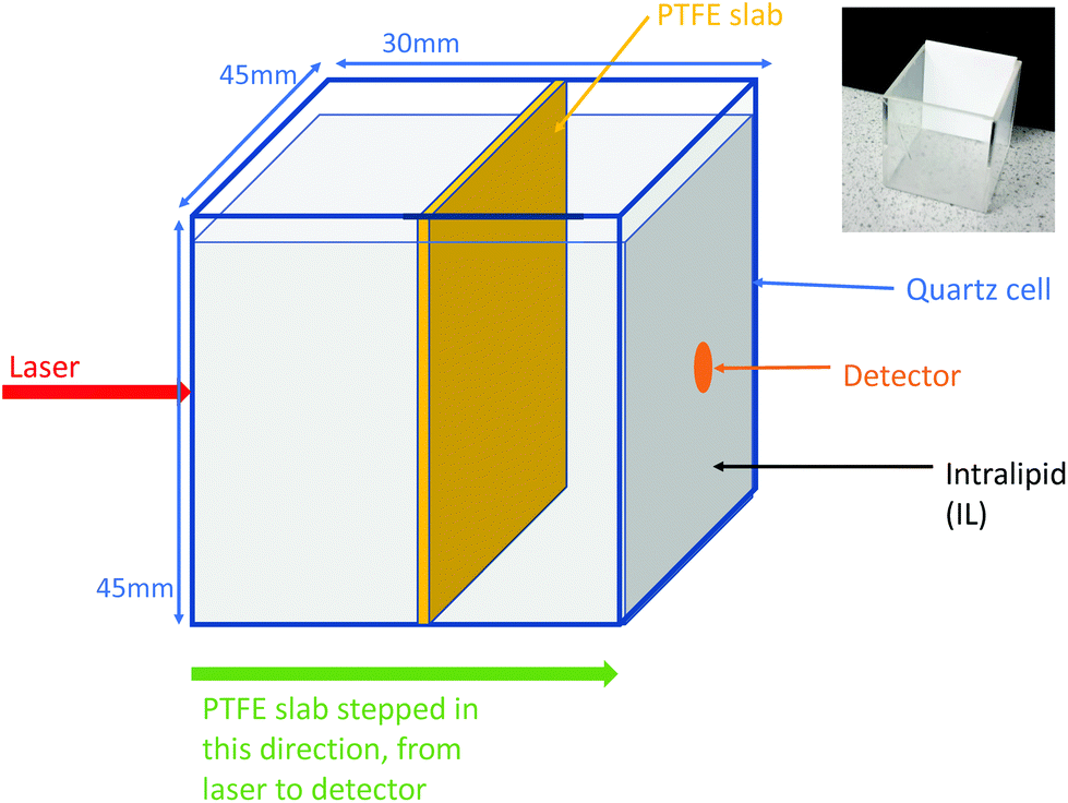Fig. 1 Liquid tissue phantom schematic with inset photo of empty quartz tank with PTFE slab inside.

The deep Raman setup at the University of Exeter used a transmission Raman configuration, as can be seen in Fig. 2. This setup has a spectrum stabilised laser (Innovative Photonics Solutions) with laser emission at 830 nm and an output power of ∼300 mW. This was coupled to a Thorlabs 105 μm multimode patch cord, then collimated and filtered by passing through two laser line filters (Semrock). These filters suppress the off-centre spectral emission from the laser line. The laser beam was brought onto the sample in a 1–2 mm diameter spot. The collimated beam passed through the sample, being scattered, absorbed and/or shifted according to the optical properties. The Raman scattered photons were then collected using an AR coated lens (f = 60 mm and diameter = 50 mm). The collimated light was then passed through a holographic super notch filter (HSPF-830.0 AR-2.0, Kaiser Optical Systems) to remove the elastically scattered light (the laser photons) and imaged onto a fibre probe bundle by an identical lens to the one used for collection. The fibre bundle (CeramOptec, “spot to slit” line type bundle assembly, active area spot diameter approximately 2 mm, slit line approximately 0.25 mm × 14.95 mm) was connected to a Holospec VPH system spectrograph (Kaiser Optical Systems). The spectra were recorded using a deep depletion CCD camera cooled to −75 °C (Andor Technology, DU420A-BR-DD, 1024 × 255 pixels). The overall spectral resolution of the system was ∼8 cm⁻¹.

Fig. 2 Diagram of the deep Raman setup used, in transmission mode. Based on a figure from Vardaki et al.¹⁰

The signal was collected using 12 accumulations of 5 seconds and the system was calibrated using Raman bands of an aspirin tablet (acetylsalicyclic acid).

Raman spectra were recorded for tissue phantoms with different IL concentrations, and therefore different scattering coefficients. Parameters such as power, wavelength, beam size and acquisition time were kept constant throughout and between mappings. The median PTFE Raman spectra are seen in Fig. 3 for each of the positions of the PTFE in the tank, with 0.25% Intralipid present as the scattering agent. Taking the median eliminated the cosmic rays present in the raw data.

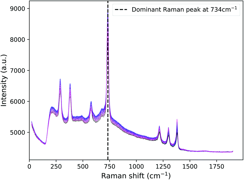Fig. 3 PTFE spectra for all positions in the tank with 0.25% Intralipid as the scattering agent. The dominant Raman peak at 734 cm⁻¹ is indicated by the dashed line.

It is clear that there is a background signal present in the spectra. Since the Monte Carlo code would only be shifting photon wavelengths according to the dominant peak, there was no need to fit and subtract all of the background signal. Instead, we clipped each spectrum around the dominant Raman peak, did a straight line fit across the base and then subtracted this. Python software was then used to fit a Gaussian peak at each position along the optical axis. Using the standard integral for a Gaussian, the area under each was calculated and plotted to show how the concentration of IL and the position of the Raman source influenced the intensity of the Raman signal detected.

2.2 Experimental outcome

Fig. 4 shows the total intensity under the dominant PTFE Raman peak for each of the concentrations of Intralipid used in the experiment: 0.25%, 0.5%, 1%, 2%, 3% and 4%. This intensity is plotted as a function of the location of the PTFE in the tank; 0 mm corresponds to the slab being in front of the laser, and 25 mm corresponds to the PTFE being in front of the detector. The units of the intensity are arbitrary as the calculation involved integrating under a Gaussian fit to the CCD output spectra. The large difference in the Raman intensities is due to higher concentrations of Intralipid decreasing the overall signal through the tank.

Fig. 4 Intensity (measured as area under the peak) of dominant Raman peak in the PTFE spectrum for each of the tested concentrations of Intralipid. The laser is incident on the tank at 0 mm, and the collection is at 25 mm. The error bars represent the shot noise from the camera.

The error bars in Fig. 4 were calculated using the guidance from the Andor camera manual, which stated the overall noise was 1.41 times the shot noise. Each count recorded by the camera was 2.5 electrons, thus giving: .

From Fig. 4, there is an evident maximum in the Raman intensity near to the middle of the tank. The concentration of the Intralipid varies the location of the peak of the Raman intensity and the shape of this peak. The lowest concentration of Intralipid gives us the strongest signal, which is to be expected as the mean free path will be longest in this instance. It is interesting to note that the peak of the Raman intensity shifts closer to the detector as the concentration of Intralipid used increases. This behaviour is discussed in the Monte Carlo results and discussion in section 3.

These results support our understanding of how Raman intensity varies with depth when the source is a “semi-infinite” slab. The peak signal appearing around the centre of the scattering volume matches previous work done by Matousek et al.³¹ and is in contrast to the finite Raman source results from Vardaki et al.¹⁰ This is in line with physical expectations: the finite source is subject to the same diffusion of laser photons, resulting in the maximum Raman photon production in front of the laser and maximum Raman photon detection probability in front of the detector. The difference arises from the fact that when in the centre, the finite source could be missed by the laser photons which can easily be scattered around it. Therefore the further from the laser that the finite Raman source is placed, the fewer laser photons will enter it and the fewer Raman photons are produced. This results in the Raman signal peaks for a finite source detecting in transmission geometry appearing in front of the laser and in front of the detector. This is the opposite result to what we have observed in this study, but both are physically correct and give insight into photon migration in turbid media and where we can expect to obtain maximum signals from.

Using the results of this experimental investigation and the understanding of how signal from a semi-infinite Raman layer behaves at different depths and optical properties, we can validate our code. The next section details the Monte Carlo numerical method employed, the optical properties required for accurate simulation, and how combining the experimental results found here with the code output can give useful insights.

3 Monte Carlo simulations

3.1 Monte Carlo method

An MCRT code was developed in Rust (a compiled, strongly typed, memory safe language similar to C++) to simulate the scattering and absorption processes present when light interacts with tissue. The code returns the number of Raman photons created and the number of those Raman photons that were detected. The incidence and detection regions are modelled to be the same as in the Experimental section. The system is able to model an arrangement of various arbitrarily shaped optical materials which are bounded by triangular meshes. These geometric objects are referred to as entities. For a more detailed description, see Jeynes et al.³² The core photon loop of the code is based upon the routine as described in Harries et al.²¹

The presented simulation is a three-dimensional cuboid-shaped domain. The tank is modelled as 26 × 41 × 41 mm (x, y, z) filled with the scattering agent. Into this, the Raman scattering layer is modelled as a 2 × 41 × 41 mm (x, y, z) entity, with the optical properties of PTFE. Two circular triangle meshes of 1 mm radius at opposite sides of the tank entity are used to describe the laser and the detector. The laser light source (located at x = 0 mm) emits photon packets at a wavelength of 830 nm; the detector mesh (located at x = 25 mm) counts the photon packets that reach it and have a wavelength of 883.9 nm. The optical properties of the IL are characterised by the scattering (μ_s) and absorption (μ_a) coefficients and are calculated from Grabtchak et al.²⁹ values for 1% IL, detailed in the optical properties section below.

The Monte Carlo simulations were optimised to replicate the experimental behaviour while not taking too long to run; they were run with the slab at locations from 3 mm to 23 mm in step sizes of 2 mm. This was a fine enough grid to show the same results as the experimental, while being coarse enough to run in a reasonable time. Large numbers of photon packets were used in order to detect sufficient signal to noise: 10⁹ photon packets for each simulation, and 10 simulations for each PTFE slab location in the tank to obtain the variance. Each concentration, therefore, is comprised of 110 simulations and took approximately 1 week to run on our 32-thread computer, with the code parallelised.

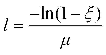
The initial direction of each packet is normal to the surface, facing into the tank along the x-direction to simulate a collimated laser beam. Following emission, the packet travels forward a random optical depth along its direction vector. This step size is described by:

where ξ is a uniform random number [0–1] and μ is the interaction coefficient of the medium the packet is currently in.

Each material in the simulation has an associated set of optical properties at the relevant wavelengths. The interaction coefficient for the medium is calculated by summation:

μ = μ_s + μ_a (2)

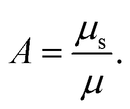
For the PTFE material that is creating Raman photon packets, this scattering coefficient is calculated by summing the elastic scattering and Raman coefficients: μ_s = μ_elastic + μ_Raman. The single scattering albedo is defined as:

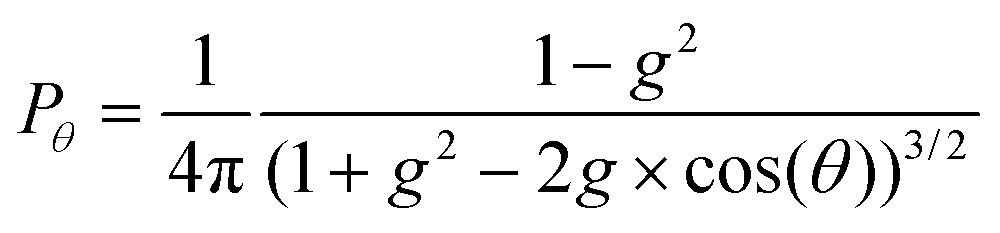
After travelling distance l, the packet then interacts with the medium through scattering. The other optical property of the medium that is required for a fully correct Monte Carlo model is the anisotropy factor (g). This variable can be any value in [−1,1] where −1 describes entirely backward scattering, 1 is for fully forward scattering and 0 is equivalent to isotropic scattering. It is used to calculate the deflection angle for the scattering packet, via the Henyey–Greenstein phase function:³³

where P_θ is a probability density function and θ is the scattering angle in radians.

We are looking at a single wavelength shift in the PTFE Raman spectrum, therefore if the photon packet has not undergone a Raman shift we use a loop to determine if it will be shifted. A random number in [0,1] is generated, and if it is less than μ_Raman/μ then the wavelength of the packet is adjusted and the optical properties are updated accordingly. The packet's statistical weight is also reduced to reflect the fraction of photons in the packet that would have been absorbed in the interaction. The remaining fraction is given by:

w′ = w × (1 − A). (5)

The photon packet will continue to propagate and scatter until it exits the domain of the simulation. In the event that its statistical weight is so small that the computational power to simulate it outweighs the contribution to the output, the packet undergoes a roulette scheme.

When a Raman scattering event occurs, the location at which it occurs is stored. This is in order to go back to this location, once the lifetime of the Raman photon has been simulated, to continue the re-weighted laser photon path as if the Raman event had not occurred. By doing this, the laser photons are not significantly depleted which is more akin to the physical experiment. This is an important consideration because if it is not implemented then the output of the Monte Carlo simulation does not match that of the experiment due to under-sampling the PTFE layer.

The Raman scattering coefficient, μ_Raman, was set to be 0.01 cm⁻¹ as this gave a good production rate of Raman packets without significantly increasing the computational time. This is several orders of magnitude greater than the realistic Raman scattering coefficient which is ∼10⁻⁶ cm⁻¹. To counteract this “over creation” of Raman photons, all of the shifted photons had correspondingly decreased weights. The dominant peak in the PTFE Raman spectrum occurs at a Raman shift of 734 cm⁻¹ which means a shifted wavelength from 830 nm (the laser wavelength) to 883.9 nm. The simulated packets were only shifted a maximum of once, and always to this wavelength. The experimental data was analysed at this peak only and so comparisons between the relative Raman intensities from the MC simulations and the experiment can be found.

3.2 Optical properties

The absorption and scattering coefficients, along with the anisotropy factor, are the dominant optical properties for a material. These have a huge impact on the output of Monte Carlo simulations and so it is vital to get them correct. For the PTFE, the optical properties were determined experimentally by time-domain diffuse spectroscopy as used in Mosca et al.:³⁴μ_a = 0.0477 cm⁻¹, μ′_s = 9.997 cm⁻¹. It is a very highly scattering medium with little absorption; this is in line with the physical properties we can observe with the eye – it is a solid, white, opaque plastic.

The optical properties of Intralipid are more difficult to determine or locate in literature, especially at the weak concentrations used in this study. Initially, the scattering coefficients used were taken from Vardaki et al.¹⁰ as the same concentrations were used in this study. The reduced scattering coefficient μ′_s was 9.2 cm⁻¹ at 1% IL, and extrapolated linearly to the other concentrations. These were originally estimated by linear extrapolation from Michels²⁸ experiments on 10%, 20% and 30% Intralipid. The optical properties did not return the expected behaviour from the experiments and were deemed inappropriate for the concentrations we are working with.

A study by Grabtchak et al.²⁹ experimentally derived the scattering coefficient and anisotropy factor for 1% IL. The anisotropy factor of g = 0.67 is in close agreement with another study at similar concentrations by Aernouts et al.²² Trying the scattering coefficients from each of these studies, only the Grabtchak value returned the behaviour from our experimental output for 1% concentration: μ_s,Grabtchak = 27.4 cm⁻¹ and μ_s,Aernouts = 5.6 cm⁻¹. Direct linear extrapolation from the Grabtchak value to the other concentrations did not return good results for the Monte Carlo output. Therefore, the code is validated against the experimental work carried out at 1% concentration of IL, and we can utilise the MC and experimental work together to derive estimates for the scattering coefficient of IL at the other concentrations. Despite not being a direct measurement of the scattering coefficient, this is a useful application of the results of our experimental and computational work.

The absorption coefficient measured for 1% IL concentration is approximately equal to that of water, meaning the Intralipid absorption is negligible at these weak concentrations compared to that of the water. The Monte Carlo simulation uses an arbitrary input laser power, and the recorded Raman signal is the sum of the weights of the detected photon packets. Therefore, to compare these outputs to detected power in our experiments, the relative behaviour of each was plotted and compared. Using both the relative behaviours, and the differences between the Raman signals at each concentration allows us to estimate the scattering coefficients.

Scattering coefficient estimates were determined by first running a large suite of Monte Carlo models: from 12 cm⁻¹ to 57.5 cm⁻¹, in step sizes of 0.1 cm⁻¹/0.2 cm⁻¹/0.5 cm⁻¹ increasing as the scattering coefficient increased. Then, the average of each of the differences between the 1% experimental output and the other concentrations’ experimental outputs were calculated. This “relative difference” was then repeated for the Monte Carlo outputs, relative to the scattering coefficient value of 27.4 cm⁻¹ (the experimentally and now computationally validated value for 1% IL concentration²⁹). These lists of relative differences were compared in order to find the scattering coefficient from the Monte Carlo suite of models that returned the corresponding relative fractional difference as seen in the experimental outputs, for each concentration. This yielded promising results, as seen in the top plot of Fig. 5, finding close matches in the fractional relative average differences which reproduce the experimental output behaviour. This fractional relative average difference means that the intensity of the dominant Raman peak for 1% Intralipid is approximately 0.8 times greater than the intensity for 4% Intralipid, as seen in Fig. 4.

Fig. 5 Top plot is the fractional comparison of the experimental average difference (purple circles) and the Monte Carlo simulation average difference (blue crosses), both performed relative to 1% Intralipid values. The lower plot is of our corresponding derived scattering coefficients against concentration. The variation in the scattering coefficient does not scale with the concentration directly as previously thought. The best fit line is the dashed line and has the formula μ_s = 5.16 × concentration(%) + 22.1. The black triangle indicates the estimated scattering coefficient for breast tissue based on our results.

The results of using the experimental differences as a basis to determine the scattering coefficients can be seen in the lower plot of Fig. 5. The derived scattering coefficient found from the suite of models is plotted against the relevant concentration. Although the relationship is linear, it is clearly not a direct scaling from concentration to scattering coefficient: the scattering coefficient does not double when the concentration is doubled. The best fit straight line yields a relationship of μ_s = 5.16 × concentration(%) + 22.1. This relationship cannot hold for all concentrations: consider a concentration of 0% as a water-filled tank, the scattering coefficient would presumably be approximately zero. However, this line appears to be a good fit for this range of Intralipid concentrations, which encompasses the scattering properties of biological tissues. The scattering coefficients were found from comparing the relative average differences of a suite of Monte Carlo models to those found in the experimental outputs and can be seen in Table 1. The reduced scattering coefficient, μ′_s, is calculated by:

μ′_s = μ_s × (1 − g)

for each of the predicted Intralipid scattering coefficients in order to compare it to values for breast tissue. The reduced scattering coefficient in uncompressed breast tissue at 830 nm has been shown to be μ′_s = 9.84 cm⁻¹.³⁵ The absorption of breast tissue has been estimated as μ_a = 0.068–0.102 cm⁻¹ for light at 825 nm in papillary breast cancer.³⁶ It should be noted that the optical properties have been shown to change with pressure applied and this change is dependent on BMI.³⁷ Using the reduced scattering coefficient allows for comparison between materials with different anisotropy values, as is the case in this study for Intralipid and breast tissue. From Table 1, it is evident that the concentration of Intralipid that most reflects breast tissue in its optical properties is 1.5%, as the breast tissue value lies between the 1% and 2% IL values derived here.

Table 1 Absorption (μ_a), scattering (μ_s), anisotropy (g), and reduced scattering coefficient (μ′_s) used in the simulations at 830 nm, the laser wavelength. The values for breast tissue^35,36 are included in order to compare with the tissue phantoms. The absorption coefficient values for the diluted IL are that of water, as this is the dominant absorbing material in the tissue phantoms

Material	μ a (cm^−1)	μ s (cm^−1)	Anisotropy (g)	μ′s (cm^−1)
PTFE	0.0477	99.97	0.9	9.997
Intralipid 0.25%	0.03	23.3	0.67	7.69
Intralipid 0.5%	0.03	25.0	0.67	8.25
Intralipid 1%	0.03	27.4	0.67	9.04
Intralipid 2%	0.03	32.5	0.67	10.7
Intralipid 3%	0.03	36.5	0.67	12.0
Intralipid 4%	0.03	43.5	0.67	14.4
Breast tissue	0.068–0.102	98.4	0.9	9.84

---

3 Results and discussion

The experimental results can be seen compared to the Monte Carlo simulation output for each concentration in Fig. 6. The simulations match the experimental output faithfully; most importantly, 1.5% Intralipid concentration has the most similar reduced scattering coefficient to breast tissue, and 1% and 2% IL experimental outputs are very well simulated by the MC code. The behaviour of the Raman intensity peak moving closer to the detector with increasing concentration is still clear when plotting relative intensity, and is replicated in the Monte Carlo results. It is clear why if we examine the physical processes at play here.

Fig. 6 A comparison of the experimental output at each concentration of Intralipid (purple) against the results of the Monte Carlo simulations (dashed teal). The scattering coefficients for the Monte Carlo simulations were calculated from the relative difference ratio and are detailed in Table 1. The laser is incident at 0 mm and the collection point is at 25 mm. Monte Carlo simulations were run with 10⁹ photon packets and repeated 10 times for each PTFE slab position in order to calculate the variance.

In lower concentrations, the Raman intensity curve has symmetry between the illumination (left) and collection (right) sides. The highest number of Raman photons are created when the PTFE block is at the illumination side as this is the point at which there are the most laser photons present in the tank, thus the highest probability for Raman scattering to occur. Once a laser photon has been converted however, it then needs to survive traversing the whole width of the tank in order to be detected. These Raman photons created with the PTFE at the illumination side have the least chance of traversing the tank without being scattered out or being absorbed. On the other side, when the PTFE block is on the right hand side of tank (and closest to the detector), Raman photons are more efficiently detected because they have the least distance to travel to the detector. However, the fewest number of Raman photons are created here as the laser photons need to survive traversing the tank of Intralipid.

The distribution of Raman signal intensity is therefore a balance between these phenomena, and the result is that the peak of this signal is somewhere near the middle of the tank. When the PTFE is at these locations, the number of laser photons reaching the block is sufficient enough to create plenty of Raman photons, and then many of these Raman photons are able to traverse the remainder of the tank to be collected. The balance shifts towards the detector as the concentration of the Intralipid increases because water absorbs Raman photons (i.e. longer wavelengths of light) more than laser photons as shown in Vardaki et al.¹⁰ The increasing scattering coefficient means the total path lengths are longer and therefore more Raman photons are absorbed between creation in the PTFE and the detector compared to lower concentrations. Thus, the maximum point of Raman signal detection moves closer to the detector as the concentration of Intralipid increases because the Raman photons have a shorter total path length and are less likely to be absorbed or exit the tank before being detected. This result is similar to what would be expected from an analytical process to solve for diffuse fluorescence with two coupled diffusion processes giving the bi-phasic outcome.³⁸

The scattering coefficients that we have determined here differ from the values found in other studies, except the value at the concentration of 1% as discussed earlier. There are limited studies, which do not always overlap (see Hohmann et al.³⁹ for an example), and did not return the experimental behaviour we have observed. At 1% IL concentration, the values found in the literature were varied: μ_s = 2.7,³⁹ 5.6,²³ 27.9 cm⁻¹ (adapted from Vardaki et al.¹⁰).

The exact reasons for the differences are outwith the scope of this study; the main difference noted here is the brand of the Intralipid used. The work by Grabtchak et al.²⁹ uses the same brand of IL (Sigma Aldritch) as used in this study, and returned a good result when used in our Monte Carlo simulations. Other studies did not return the expected results, and used different brands of IL. As IL is not manufactured specifically to have identical scattering coefficients, this could go some way to explaining the differences observed. Another important factor is the length of time taken to do the experiments. IL is a lipid emulsion, therefore over time there can be quality degradation due to the fat droplets joining together. Our experimental work was completed in 2 days from opening the bottle in order to minimise this effect but it is unclear how long other studies have taken. There was no noticeable degradation or change in the IL over the 2 days of the experimental work. The length of time to complete the work could have an effect on the optical properties determined by different studies. Additionally, the difference in the phantom volumes used could play a role, especially pertaining to boundary conditions.

Our Monte Carlo numerical tool replicates the behaviour seen in the experimental results and is also capable of gaining information about the optical properties of the tissue phantoms by use of the experimental outputs. This information can then in turn be used to inform future experiments: this reduces costs by predicting experimental outcomes and simulating far more environments and Raman material distributions than currently readily available in a physical laboratory.

4 Conclusions

Experimentally, we have explored the Raman scattering distribution in liquid tissue phantoms in order to validate our Monte Carlo numerical tool. These tissue phantoms are useful because they approximately mimic the scattering properties of breast tissue. It has clearly been shown how the intensity of the Raman signal varies as the scattering coefficient of the liquid phantom changes. The results show that for a “semi infinite” layer of Raman scattering material, the highest signals are likely to be from the layers nearer the middle of the material using transmission Raman. This is contrary to earlier observations with a finite vial containing the Raman material, which showed a stronger signal from the illumination and collection surfaces and the weakest signal in the middle. These results are in line with previous studies and strengthen our understanding of light transport in these situations.

In this study, we have shown that our Monte Carlo numerical tool with the library arctk is capable of reproducing experimental results. We have recovered the same behaviour in our simulated photon packets as was recorded in the experimental outcomes: a strongest signal in the middle of the phantom, with this peak shifting towards the detector for more turbid media. Using experimentally derived optical properties as our input, this has validated the code. This shows promise for future applications of Monte Carlo simulations in the journey to improve breast cancer detection.

Crucially, we have found that assuming direct linear extrapolation for the scattering coefficient between different concentrations of Intralipid may not be physically valid, in the most dilute regimes. A linear relationship does exist, with a shallow gradient. By looking at the differences between the experimental outputs, we have found more realistic scattering coefficients for Intralipid at a variety of concentrations and proven that the new values return the observed signal behaviour.

Simulations can investigate a variety of future probe designs and realistic calcification distributions. In this way, we will be able to rule out sub-optimal setups and ultimately work towards a non-invasive deep Raman diagnosis of breast cancer.

Author contributions

The author contributions are detailed below, as defined by CRediT. L. J. M.: Formal analysis, investigation, software, visualisation, writing – original draft. F. W.: Software, data curation. B. G.: Methodology, investigation. N. S.: Conceptualisation, methodology, resources, supervision, writing – review and editing. T. J. H.: Conceptualisation, methodology, resources, supervision, writing – review and editing.

Conflicts of interest

There are no conflicts to declare.

Acknowledgements

L. J. M. acknowledges the support of an EPSRC studentship funded through grant [EP/M506527/1]. N. S. and B. G. were supported by [EP/P012442/1] and [EP/R020965/1]. We thank Pavel Matousek for his valuable discussions and Sara Mosca for her experimental work to determine the optical properties of this slab of PTFE.

References

1. L. Kiefert, P. Colomban, D. De Faria, L. Burgio, D. C. Smith, P. S. Middleton, M. Bouchard, I. Freestone, D. A. Long, P. Vandenabeele, G. di Lonardo, F. Perez, D. Bersani, R. Withnall, C. Coupry, E. M. Castellucci, A. Middleton, P. P. Lottici, A. Casoli, P. Wyeth, S. E. J. Bell, J.-P. Chalain, S. Haberli, S. Bruni, L. Robinet and D. Thickett, Raman Spectroscopy in Archaeology and Art History, The Royal Society of Chemistry, 2005.
2. K. Buckley and P. Matousek, Recent advances in the application of transmission Raman spectroscopy to pharmaceutical analysis, J. Pharm. Biomed. Anal., 2011, 55, 645–652.
3. E. E. Lawson, B. W. Barry, A. C. Williams and H. G. M. Edwards, Biomedical Applications of Raman Spectroscopy, J. Raman Spectrosc., 1997, 28, 111–117.
4. Cancer statistics, http://cancerresearchuk.org/health-professional/.
5. E. D. Pisano, C. Gatsonis, E. Hendrick, M. Yaffe, J. K. Baum, S. Acharyya, E. F. Conant, L. L. Fajardo, L. Bassett, C. D'Orsi, R. Jong and M. Rebner, Diagnostic Performance of Digital versus Film Mammography for Breast-Cancer Screening, N. Engl. J. Med., 2005, 353, 1773–1783.
6. C. K. Kuhl, S. Schrading, C. C. Leutner, N. Morakkabati-Spitz, E. Wardelmann, R. Fimmers, W. Kuhn and H. H. Schild, Mammography, Breast Ultrasound, and Magnetic Resonance Imaging for Surveillance of Women at High Familial Risk for Breast Cancer, J. Clin. Oncol., 2005, 23, 8469–8476.
7. R. Blanks, R. Given-Wilson, R. Alison, J. Jenkins and M. Wallis, An analysis of 11.3 million screening tests examining the association between needle biopsy rates and cancer detection rates in the English NHS Breast Cancer Screening Programme, Clin. Radiol., 2019, 74, 384–389.
8. L. Frappart, M. Boudeulle, J. Boumendil, H. C. Lin, I. Martinon, C. Palayer, Y. Mallet-Guy, D. Raudrant, A. Bremond, Y. Rochet and J. Feroldi, Structure and composition of microcalcifications in benign and malignant lesions of the breast: Study by light microscopy, transmission and scanning electron microscopy, microprobe analysis, and X-ray diffraction, Hum. Pathol., 1984, 15, 880–889.
9. C. M. Büsing, U. Keppler and V. Menges, Differences in microcalcification in breast tumors, Virchows Arch. A: Pathol. Anat. Histol., 1981, 393, 307–313.
10. M. Z. Vardaki, B. Gardner, N. Stone and P. Matousek, Studying the distribution of deep Raman spectroscopy signals using liquid tissue phantoms with varying optical properties, Analyst, 2015, 140, 5112–5119.
11. F. W. L. Esmonde-White, K. A. Esmonde-White, M. R. Kole, S. A. Goldstein, B. J. Roessler and M. D. Morris, Biomedical tissue phantoms with controlled geometric and optical properties for Raman spectroscopy and tomography, Analyst, 2011, 136, 4437–4446.
12. J.-L. H. Demers, F. W. Esmonde-White, K. A. Esmonde-White, M. D. Morris and B. W. Pogue, Next-generation Raman tomography instrument for non-invasive in vivo bone imaging, Biomed. Opt. Express, 2015, 6, 793–806.
13. I. E. Iping Petterson, F. W. L. Esmonde-White, W. de Wilde, M. D. Morris and F. Ariese, Tissue phantoms to compare spatial and temporal offset modes of deep Raman spectroscopy, Analyst, 2015, 140, 2504–2512.
14. I. A. Matveeva, O. O. Myakinin, Y. A. Khristoforova, I. A. Bratchenko, A. A. Moryatov, S. V. Kozlov and V. P. Zakharov, Tissue Optics and Photonics, 2020, pp. 194–200.
15. N. Everall, T. Hahn, P. Matousek, A. W. Parker and M. Towrie, Photon Migration in Raman Spectroscopy, Appl. Spectrosc., 2004, 58, 591–597.
16. M. D. Keller, R. H. Wilson, M.-A. Mycek and A. Mahadevan-Jansen, Monte Carlo Model of Spatially Offset Raman Spectroscopy for Breast Tumor Margin Analysis, Appl. Spectrosc., 2010, 64, 607–614.
17. V. Periyasamy, S. Sil, G. Dhal, F. Ariese, S. Umapathy and M. Pramanik, Experimentally validated Raman Monte Carlo simulation for a cuboid object to obtain Raman spectroscopic signatures for hidden material, J. Raman Spectrosc., 2015, 46, 669–676.
18. V. Periyasamy, H. B. Jaafar and M. Pramanik, Optical Interactions with Tissue and Cells XXIX, 2018, pp. 107–112.
19. S. Wang, J. Zhao, H. Lui, Q. He, J. Bai and H. Zeng, Monte Carlo simulation of in vivo Raman spectral Measurements of human skin with a multi-layered tissue optical model, J. Biophotonics, 2014, 7, 703–712.
20. P. Matousek, M. D. Morris, N. Everall, I. P. Clark, M. Towrie, E. Draper, A. Goodship and A. W. Parker, Numerical Simulations of Subsurface Probing in Diffusely Scattering Media Using Spatially Offset Raman Spectroscopy, Appl. Spectrosc., 2005, 59, 1485–1492.
21. T. Harries, T. Haworth, D. Acreman, A. Ali and T. Douglas, The TORUS radiation transfer code, 2019.
22. B. Aernouts, E. Zamora-Rojas, R. V. Beers, R. Watté, L. Wang, M. Tsuta, J. Lammertyn and W. Saeys, Supercontinuum laser based optical characterization of Intralipid® phantoms in the 500–2250 nm range, Opt. Express, 2013, 21, 32450–32467.
23. B. Aernouts, R. V. Beers, R. Watté, J. Lammertyn and W. Saeys, Dependent scattering in Intralipid® phantoms in the 600–1850 nm range, Opt. Express, 2014, 22, 6086–6098.
24. P. Di Ninni, F. Martelli and G. Zaccanti, Intralipid: towards a diffusive reference standard for optical tissue phantoms, Phys. Med. Biol., 2010, 56, 21.
25. P. D. Ninni, F. Martelli and G. Zaccanti, Effect of dependent scattering on the optical properties of Intralipid tissue phantoms, Biomed. Opt. Express, 2011, 2, 2265–2278.
26. G. Zaccanti, S. D. Bianco and F. Martelli, Measurements of optical properties of high-density media, Appl. Opt., 2003, 42, 4023–4030.
27. H. J. van Staveren, C. J. M. Moes, J. van Marie, S. A. Prahl and M. J. C. van Gemert, Light scattering in lntralipid-10% in the wavelength range of 400–1100 nm, Appl. Opt., 1991, 30, 4507–4514.
28. R. Michels, F. Foschum and A. Kienle, Optical properties of fat emulsions, Opt. Express, 2008, 16, 5907–5925.
29. S. Grabtchak, T. Palmer, F. Foschum, A. Liemert, A. Kienle and W. Whelan, Experimental spectro-angular mapping of light distribution in turbid media, J. Biomed. Opt., 2012, 17, 067007.
30. F. Sardanelli, F. Zandrino, A. Imperiale, E. Bonaldo, M. G. Quartini and N. Cogorno, Breast Biphasic Compression versus Standard Monophasic Compression in X-ray Mammography, Radiology, 2000, 217, 576–580.
31. P. Matousek and A. W. Parker, Bulk Raman Analysis of Pharmaceutical Tablets, Appl. Spectrosc., 2006, 60, 1353–1357.
32. J. C. G. Jeynes, F. Wordingham, L. J. Moran, A. Curnow and T. J. Harries, Monte Carlo Simulations of Heat Deposition during Photothermal Skin Cancer Therapy Using Nanoparticles, Biomolecules, 2019, 9, 343.
33. L. G. Henyey and J. L. Greenstein, Diffuse radiation in the Galaxy, Astrophys. J., 1941, 93, 70–83.
34. S. Mosca, P. Lanka, N. Stone, S. K. V. Sekar, P. Matousek, G. Valentini and A. Pifferi, Optical characterization of porcine tissues from various organs in the 650–1100nm range using time-domain diffuse spectroscopy, Biomed. Opt. Express, 2020, 11, 1697–1706.
35. S. L. Jacques, Optical properties of biological tissues: a review, Phys. Med. Biol., 2013, 58, R37–R61.
36. S. Fantini, S. A. Walker, M. A. Franceschini, M. Kaschke, P. M. Schlag and K. T. Moesta, Assessment of the size, position, and optical properties of breast tumors in vivo by noninvasive optical methods, Appl. Opt., 1998, 37, 1982–1989.
37. S. Jiang, B. W. Pogue, K. D. Paulsen, C. Kogel and S. Poplack, In vivo near-infrared spectral detection of pressure-induced changes in breast tissue, Opt. Lett., 2003, 28, 1212–1214.
38. D. Piao, A. Zhang and G. Xu, Photon diffusion in a homogeneous medium bounded externally or internally by an infinitely long circular cylindrical applicator. V. Steady-state fluorescence, J. Opt. Soc. Am. A, 2013, 30, 791–805.
39. M. Hohmann, B. Lengenfelder, D. Muhr, M. Späth, M. Hauptkorn, F. Klämpfl and M. Schmidt, Direct measurement of the scattering coefficient, Biomed. Opt. Express, 2021, 12, 320–335.

---

Footnote

† The library can be found at https://github.com/FreddyWordingham/arctk.

---