
 Open Access Article
 This Open Access Article is licensed under a
 Creative Commons Attribution 3.0 Unported Licence
Mid-infrared spectral classification of endometrial cancer compared to benign controls in serum or plasma samples†
David
Mabwa
 *a,
Ketankumar
Gajjar
b,
David
Furniss
a,
Roberta
Schiemer
b,
Richard
Crane
a,
Christopher
Fallaize
c,
Pierre L.
Martin-Hirsch
d,
Francis L.
Martin
e,
Theordore
Kypraios
c,
Angela B.
Seddon
a and
Sendy
Phang
a
*a,
Ketankumar
Gajjar
b,
David
Furniss
a,
Roberta
Schiemer
b,
Richard
Crane
a,
Christopher
Fallaize
c,
Pierre L.
Martin-Hirsch
d,
Francis L.
Martin
e,
Theordore
Kypraios
c,
Angela B.
Seddon
a and
Sendy
Phang
a
aMid-Infrared Photonics Group, George Green Institute for Electromagnetics’ Research, Faculty of Engineering, University of Nottingham, Nottingham NG7 2RD, UK. E-mail: david.mabwa@nottingham.ac.uk; sendy.phang@nottingham.ac.uk
bObstetrics and Gynaecology, Nottingham University Hospitals NHS Trust – City Campus, Nottingham City Hospital, Hucknall Road, Nottingham, NG5 1PB, UK
cSchool of Mathematical Sciences, The Mathematical Sciences Building, University Park, University of Nottingham, NG7 2RD, UK
dLancashire Teaching Hospitals, UK
eBiocel UK Ltd, Hull HU10 7TS, UK
First published on 29th July 2021
Abstract
This study demonstrates a discrimination of endometrial cancer versus (non-cancerous) benign controls based on mid-infrared (MIR) spectroscopy of dried plasma or serum liquid samples. A detailed evaluation was performed using four discriminant methods (LDA, QDA, kNN or SVM) to execute the classification task. The discriminant methods used in the study comprised methods that are widely used in the statistics (LDA and QDA) and machine learning literature (kNN and SVM). Of particular interest, is the impact of discrimination when presented with spectral data from a section of the bio-fingerprint region (1430 cm−1 to 900 cm−1) in contrast to the more extended bio-fingerprint region used here (1800 cm−1 to 900 cm−1). Quality metrics used were the misclassification rate, sensitivity, specificity, and Matthew's correlation coefficient (MCC). For plasma (with spectral data ranging from 1430 cm−1 to 900 cm−1), the best performing classifier was kNN, which achieved a sensitivity, specificity and MCC of 0.865 ± 0.043, 0.865 ± 0.023 and 0.762 ± 0.034, respectively. For serum (in the same wavenumber range), the best performing classifier was LDA, achieving a sensitivity, specificity and MCC of 0.899 ± 0.023, 0.763 ± 0.048 and 0.664 ± 0.067, respectively. For plasma (with spectral data ranging from 1800 cm−1 to 900 cm−1), the best performing classifier was SVM, with a sensitivity, specificity and MCC of 0.993 ± 0.010, 0.815 ± 0.000 and 0.815 ± 0.010, respectively. For serum (in the same wavenumber range), QDA performed best achieving a sensitivity, specificity and MCC of 0.852 ± 0.023, 0.700 ± 0.162 and 0.557 ± 0.012, respectively. Our findings demonstrate that even when a section of the bio-fingerprint region has been removed, good classification of endometrial cancer versus non-cancerous controls is still maintained. These findings suggest the potential of a MIR screening tool for endometrial cancer screening.
1. Introduction
Endometrial cancer (EC) is the 4th most frequently diagnosed gynaecological malignancy in the first world, and also the 4th most common cancer to affect women in the UK.1,2 In 2018, >382![[thin space (1/6-em)]](https://www.rsc.org/images/entities/char_2009.gif) 000 women were diagnosed with EC, and approximately 90000 fatalities were recorded worldwide.3 In 2020, the number of new EC cases increased to >417300, with recorded deaths also increasing to >97000.4 Despite this, widespread screening of EC is not currently advocated. This is primarily due to the notably low specificity (ranging from 36% to 68% (ref. 5)) and low positive predictive values (ranging from 4% (ref. 6) to 9.6% (ref. 7)), caused by screening subjectivity arising from the high dependence on the operator's experience, when using the most common screening method (i.e., transvaginal ultrasonography (TVS)).8
000 women were diagnosed with EC, and approximately 90000 fatalities were recorded worldwide.3 In 2020, the number of new EC cases increased to >417300, with recorded deaths also increasing to >97000.4 Despite this, widespread screening of EC is not currently advocated. This is primarily due to the notably low specificity (ranging from 36% to 68% (ref. 5)) and low positive predictive values (ranging from 4% (ref. 6) to 9.6% (ref. 7)), caused by screening subjectivity arising from the high dependence on the operator's experience, when using the most common screening method (i.e., transvaginal ultrasonography (TVS)).8
Developing new, more effective evidence-based screening methods for the early detection of gynaecological cancers has been the focus of oncology researchers.9,10 One such method is through the use of sensitive and specific biomarkers found in dried biofluids such as plasma, serum, urine, or saliva.11 DNA/RNA is an example of a potential biomarker found in the plasma or serum of cancer patients at higher levels when compared to non-cancerous patients.12,13 This DNA/RNA is present in blood due to mechanisms such as tumour necrosis,14 apoptosis15 and active release.16 Additionally, tumour cells found circulating in the peripheral blood of cancer patients (with levels ranging from 1:103 to 1:107 nucleated cells in blood17), once identified, could be used as cancer biomarkers.18
The limitations of the current methods for screening and diagnostic methods mentioned above, has led to a growing research interest to apply mid-infrared (MIR) spectroscopy for assisting in the diagnosis of EC, due to its ability to detect minute changes in the chemistry of bio-samples.11
MIR spectroscopy works by identifying the presence and distribution of biomolecules within a bio-sample. When a bio-sample (biofluid or tissue) absorbs MIR radiation (4000–200 cm−1 (ref. 19)), covalently bound molecular species vibrate at their characteristic frequency with greater amplitude; absorption intensity is related to their quantity, i.e., concentration, and wavelength is related to the nature of their bonding.20 Within the bio-fingerprint region (1800–900 cm−1 (ref. 21 and 22)) of the MIR range, there exist the fundamental frequencies of various biomolecules of interest. Proteins are known to primarily contribute to absorption bands found at 1650 cm−1 to 1665 cm−1, 1550 cm−1 and 1310 cm−1 to 1200 cm−1, which are assigned to Amide I (C![[double bond, length as m-dash]](https://www.rsc.org/images/entities/char_e001.gif) O stretching), Amide II (N–H bending, C–H stretching, C–O bending and C–C and N–C stretching) and Amide III (C–H/N–H deformation), respectively. Lipids contribute to bands at 1467 cm−1 to 1400 cm−1 (C–H scissoring or CH2 and CH3 and CO stretching of –COO−), and at ∼1070 cm−1 (C–O–C, CO–O–C symmetric (sym) stretching).23 Bands attributed to carbohydrates are found at 1173 cm−1, 1154 cm−1 (symmetric stretching of C–O, coupled to C–O–H bending), 1041 cm−1 and 1055 cm−1 (sym C–O–C stretching) and 1023 cm−1 (sym C–O stretching). Finally, bands attributed to nucleic acids, phospholipids and nucleotides are found at ∼1250 cm−1 to 1220 cm−1 (asymmetric (asym) PO stretching in PO2−), ∼1085 cm−1 (sym PO stretching in PO2 and sym CO–O–C stretching), and ∼900 cm−1 to 800 cm−1 (CC, CN and C–H vibrations in ring structure).23
O stretching), Amide II (N–H bending, C–H stretching, C–O bending and C–C and N–C stretching) and Amide III (C–H/N–H deformation), respectively. Lipids contribute to bands at 1467 cm−1 to 1400 cm−1 (C–H scissoring or CH2 and CH3 and CO stretching of –COO−), and at ∼1070 cm−1 (C–O–C, CO–O–C symmetric (sym) stretching).23 Bands attributed to carbohydrates are found at 1173 cm−1, 1154 cm−1 (symmetric stretching of C–O, coupled to C–O–H bending), 1041 cm−1 and 1055 cm−1 (sym C–O–C stretching) and 1023 cm−1 (sym C–O stretching). Finally, bands attributed to nucleic acids, phospholipids and nucleotides are found at ∼1250 cm−1 to 1220 cm−1 (asymmetric (asym) PO stretching in PO2−), ∼1085 cm−1 (sym PO stretching in PO2 and sym CO–O–C stretching), and ∼900 cm−1 to 800 cm−1 (CC, CN and C–H vibrations in ring structure).23
Although MIR spectroscopy is able to detect subtle changes in the chemistry of bio-samples, the accurate classification of these data heavily depends on the development and application of data processing and classifier tools. There are three main stages involved in data processing: (1) pre-processing; (2) feature extraction (FE); and (3) classification. When applied to spectral data, the pre-processing stage aims to reduce/remove the contribution of information that is not related to the bio-sample, thereby increasing the interpretability of the data, and enhancing the accuracy and robustness of ensuing multivariate analyses. This stage corrects for physical interferences such as light scattering due to varying particle sizes, and sample thicknesses. Random instrument noise is also corrected for during this step.24 The pre-processing stage involves two main procedures: spectral data smoothing and correction.
Smoothing/de-noising is accomplished via the use of spectral filters that eliminate random noise, while retaining important spectral information. The most common technique currently used is the Savitzky–Golay (SG) algorithm.25 Other commonly used techniques include wavelet de-noising26 and minimum noise fraction.27 Spectral correction involves multiple techniques (light-scattering correction, baseline correction, spectral differentiation, and normalisation) that may be applied in sequence depending on the nature of the dataset and the aims of the investigator. If data collection is accomplished via near-IR (NIR) spectroscopy, then light-scattering correction needs to be undertaken as light scattering (Mie scattering) is a very common artefact in NIR spectroscopy;28 it also may occur in MIR spectroscopy, especially in cytology, and can cause further complications due to resonant effects.29 Some techniques, such as standard normal variate (SNV) and multiplicative scatter correction (MSC) can be used to correct for this artefact.30 Baseline correction (BC), another spectral correction technique, is used to eliminate interferences that result from background absorption. The main techniques used for BC are rubber-band-like BC, Whittaker filter, automatic weighted squares, asymmetric least squares, and polynomial BC.24,31 Spectral differentiation can also be applied to spectral data to simultaneously correct for baseline distortion and light scattering; whilst this is not the case for Resonant scattering, it is inferred that such oscillatory spectral effects will be very small here due to the nature of the samples taken.29 Spectral normalisation is commonly applied to IR spectral data to correct for varying sample concentration or thickness. The most common techniques for normalising IR data is Amide I and vector normalisation. The review paper24 provides an excellent summary of various pre-processing procedures that can be applied to spectral data.
Feature extraction (FE) forms an essential data decomposition step that helps identify clustering patterns in the data, allowing for initial conclusions to be drawn about the sample nature, potential outliers, and experimental errors. The most common FE method is principal component analysis (PCA). During PCA, spectral data are decomposed into a few principal components (PCs) that account for the greatest variance in the original dataset.31
There are two types of classifiers, unsupervised and supervised. Unsupervised classification (clustering) works by classifying data into classes based on a distance measure without user-supplied class grouping information. Examples include k-means clustering and hierarchical cluster analysis.32 Supervised classification/machine learning techniques, however, involve classifying input pre-processed spectral data into classes based on training data. Popular techniques are discriminant analysis (linear (LDA) or quadratic (QDA)), k-nearest neighbour (kNN), support vector machines (SVM), artificial neural networks (ANN) and Bayesian-based inference methods.24,31 Studies have been conducted on the distinction of cancerous samples from control samples through the use of MIR spectroscopy on biofluids in breast cancer,33 bladder cancer,34 brain cancer,35 oesophageal cancer,36 ovarian cancer and endometrial cancer.17
Among the first to use and analyse human serum with transmission MIR spectroscopy to diagnose breast cancer was Backhaus et al.33 In this study, serum samples from 98 breast cancer patients with carcinomas ranging from 2 mm to 2 cm in diameter, and 98 healthy controls were used. They used 1 μL of serum for each patient, diluted with 3 μL of distilled water and dried onto a Si-plate. After pre-processing the generated data (via vector normalisation, spectral 2nd order derivation, and SG filtering), the data were classified using two independent classifiers, cluster analysis or ANN. Backhaus et al. found that both classifiers were able to produce sensitivity and specificity results >90% (cluster analysis: sensitivity = 96%, specificity = 93%; ANN: sensitivity = 95%, specificity = 95%). In a study by Maitra et al.,36 the diagnostic power of PCA-QDA, successive projection algorithm: SPA-QDA and genetic algorithm: GA-QDA for different classes of oesophageal cancer (inflammation, Barrett's oesophagus, low- or high-grade dysplasia and oesophageal adenocarcinoma) were tested on spectral data collected from dried plasma, serum, saliva, and urine samples using attenuated total reflection Fourier-transform IR (ATR-FTIR) spectroscopy. The data were initially pre-processed by cutting between 1800 cm−1 and 900 cm−1, baseline corrected using the rubber band method, and normalised to the Amide I peak (1650 cm−1). They found that the diagnostic power of GA-QDA was strongest on plasma (sensitivity and specificity = 100%, in all disease states) and serum (sensitivity ranging from 95.6% to 100%, and specificity ranging from 50% to 100%, with a median value of 92.85%) datasets. Similarly, Gajjar et al.17 used ATR-FTIR spectroscopy to analyse dried plasma and serum samples of patients diagnosed with ovarian cancer. They found that a classification rate of 96.67% ± 7.03% was produced when the feature selection method, LASSO (least absolute shrinkage and selection operator) was paired with the eClass algorithm (evolving Classifier)37 to classify ovarian plasma data, while a classification rate of 95% ± 8.05% was produced when forward feature selection (FFS) was paired with kNN to classify ovarian serum data. This shows that MIR spectral analysis of biofluids paired with machine learning (ML) techniques offers a promising non- to minimally invasive route to the accurate diagnosis of various cancers.
The main aim of the present study was to explore the efficacy of different combinations of pre-processing procedures and discrimination methods to differentiate the MIR spectroscopic spectra between cancerous (plasma and serum from patients with endometrial cancer diagnosis) and non-cancerous control samples. The spectral data used in this are identical to those used by Gajjar et al.17 There are, however, differences in the processing method, from the earlier work. Firstly, the training and test data were strictly separated (see section 2.2). Secondly, in acknowledgement of future in vivo application of diagnosis by means of MIR vibrational spectral determination, the water-free part of the spectrum (1430 cm−1 to 900 cm−1) was analysed in addition to the previously used span of 1800 cm−1 to 900 cm−1 (the former excludes the Amide I and II bands at 1650 cm−1 and 1550 cm−1, respectively). Finally, pre-processing is that spectral data are not baseline corrected using the rubber band-like method, but instead are filtered using the Savitzky–Golay method, to the 5th polynomial and differentiated to the 1st order; data then underwent PCA before classification methods were applied the dataset was split into 70% training and 30% testing sets ensuring an objective validation of the classifiers’ performance against unseen datasets. The datasets were then passed into multiple classification algorithms: LDA, QDA, kNN or SVM. The performance of each classifier was assessed by the misclassification rate, sensitivity, specificity, and the Matthew's correlation coefficient (MCC).
2. Materials and methods
2.1. Sample preparation
Human blood samples were collected [Research and Ethics Committee (REC) approval no.: 10/H0308/75] from 126 patients [31 endometrial plasma cancer (EPCan) patients, 32 endometrial plasma control (EPCon), 30 endometrial serum cancer (ESCan) patients, and 33 endometrial serum control (ESCon) patients] prior to surgery. In this study, none of the patients in the cancer or control class had ovarian cancer. When selecting participants, a second tumour was an exclusion criterion. In the original paper,17 ovarian cancer and endometrial cancer were both investigated. The current work utilised data only from the endometrial cancer patients. All blood samples were collected from patients prior to any and all therapies, treatments, and surgeries. See ref. 17 for more details.The blood samples underwent centrifugation for 15 min at 300 rpm to separate the erythrocytes from serum (−EDTA) or plasma (+EDTA). The samples were then stored at −85 °C in cryogenic tubes until analysis. Prior to ATR-FTIR spectrochemical analysis, the frozen samples were thawed at ambient temperature and 100 μL of plasma or serum was decanted and transferred onto different IR-reflective glass slides (Kevley Technologies) and air-dried for 1 h.
2.2. ATR-FTIR spectroscopy protocol
MIR spectral data were obtained using the Bruker Tensor 27 FTIR with the Helios attachment. To collect spectral data, slides with the dried plasma or serum samples were placed atop a vertically movable stage, which was underneath the diamond crystal. The slides were raised until good contact between the sample and diamond crystal was achieved, then a spectrum was collected. Spectral data were collected from 20 different spatial locations per sample and the diamond ATR crystal cleaned between each sample. A total number of 2520 spectra (from all 126 patients’ samples) were collected (620 EPCan dataset, 640 EPCon dataset, 600 ESCan dataset and 660 ESCon dataset). These datasets were then combined to form the “Endometrial Plasma” dataset (containing both EPCan and EPCon datasets of 1260 spectra) and the “Endometrial Serum” dataset (also containing both ESCan and ESCon datasets of 1260 spectra).Hold-out cross validation was implemented in this work, such that the spectral datasets (i.e., “Endometrial Plasma” and “Endometrial Serum”) were split for training and testing sets in a 7:3 ratio as in Table 1. This separation was completed manually so that all spectral data from each patient were either in the training or testing group. This is because a random separation resulted in the presence of spectral data from a single patient, in both the training and testing groups.
:3 split was achieved by splitting the patients and not the individual spectra
| Endometrial Plasma (n) | Endometrial Serum (n) | ||
|---|---|---|---|
| Training spectra | Cancer | 440 | 420 |
| Control | 440 | 460 | |
| Testing spectra | Cancer | 180 | 180 |
| Control | 200 | 200 |
2.3. Data processing
The data import, pre-treatment techniques, the assembly of chemometric classification classifiers and statistical analyses were all implemented in MATLAB R2020b software (MathWorks, USA) (Fig. 1).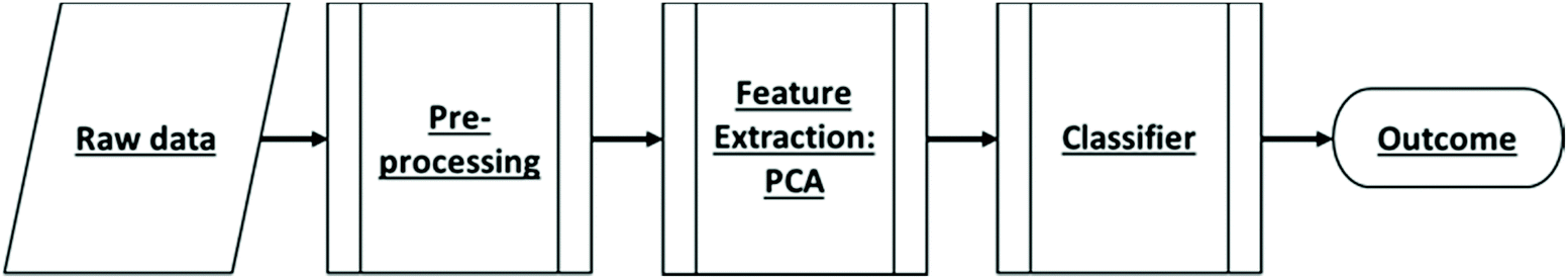 | ||
| Fig. 1 Block diagram of describing the classification procedures of the MIR spectroscopic datasets. | ||
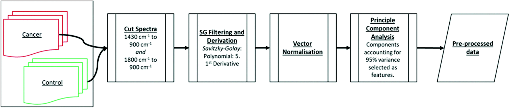 | ||
| Fig. 2 Overview of the steps involved in pre-processing and feature selection. | ||
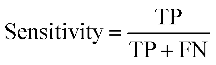 | (1) |
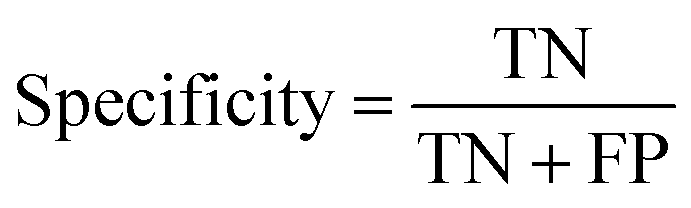 | (2) |
 | (3) |
| MR = 1 − Accuracy | (4) |
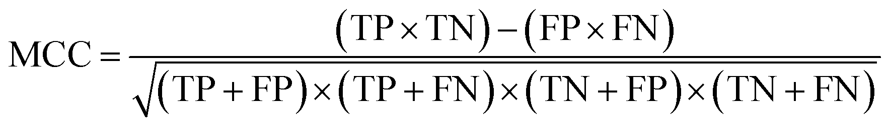 | (5) |
The value of MCC can range from −1 to 1. An MCC of 1 indicates a perfect classifier (FP + FN = 0). An MCC of −1 indicates a classifier that incorrectly discriminates all classes (TP + TN = 0). An MCC of 0 indicates a classifier that classifies at an accuracy equivalent to the flip of a coin, i.e., accuracy of 50%. See Fig. 3 for a schematic description of the methods performed in this study.
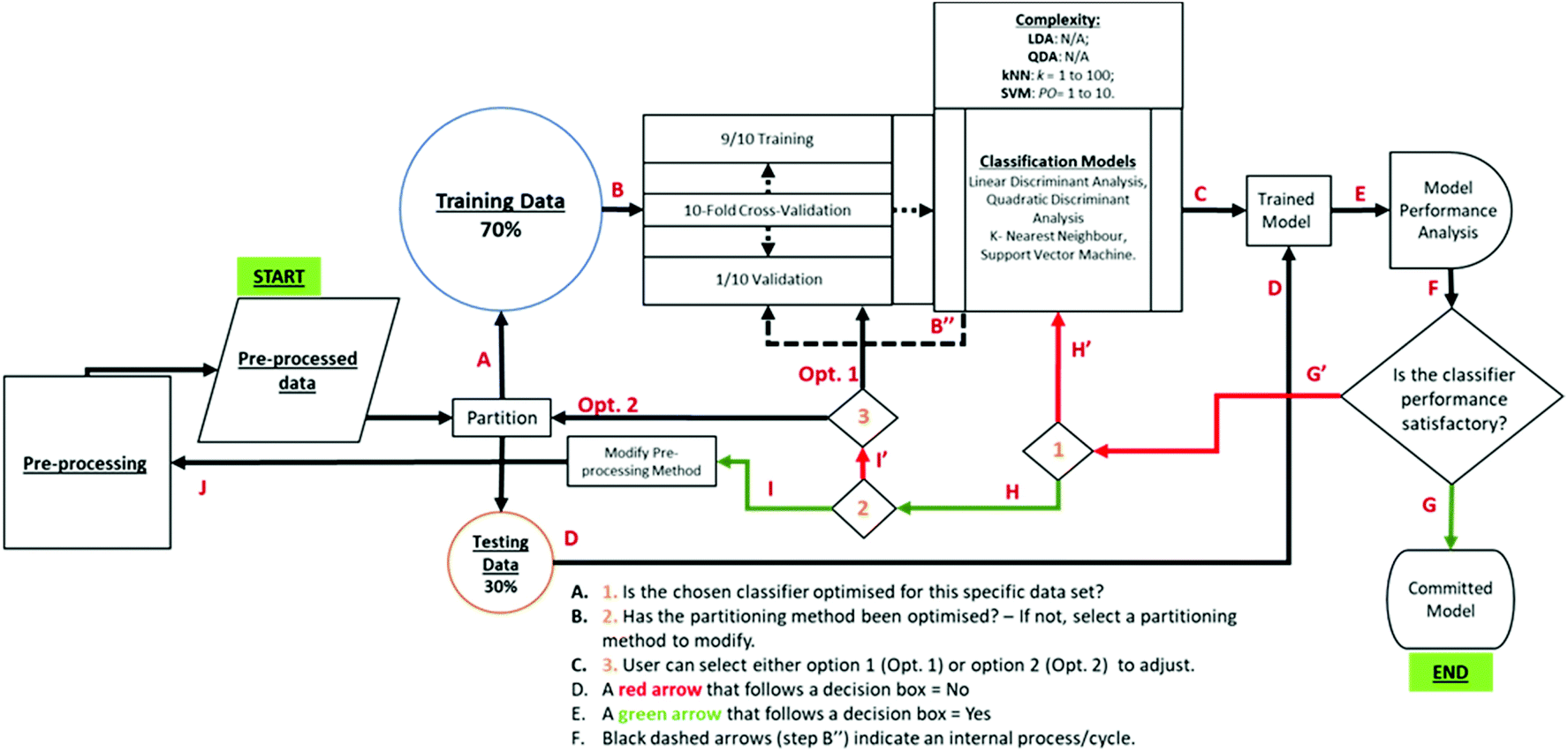 | ||
| Fig. 3 Block diagram of the methodology employed in this study. (A) The pre-processed data are partitioned into a testing and training sets. (B) The training data is then passed into a 10-fold internally cross validated classification algorithm (either LDA, QDA, kNN or SVM). (B′′) Step B is repeated 10 times, accounting for the number of folds specified. (C) This produces a trained classifier. (D) The classifier is tested with the testing data, that have undergone the same pre-processing steps as the training set and (E). Analysed with various quality metrics (sensitivity, specificity, misclassification rate, and Matthew's correlation coefficient). (F) If the classifier performance is satisfactory, (G). A committed model is produced. (G′) If the model is not satisfactory, 〈1〉. Check whether the classifier parameters have been optimised for this dataset. If not, (H′). Optimise each classifier until performance improves. (H). If classifier parameters have been optimised, 〈2〉. Check whether the partitioning method has been optimised. (I′) If not 〈3〉 alter either the cross-validation method within each model (Opt.1) or the partitioning percentages (Opt. 2). If (I), the partitioning method has been optimised, (J). Modify the pre-processing method. | ||
3. Results
As described in section 2.3., herein, we evaluate the diagnostic capability of classifiers when inputted with MIR spectral data from two sections of the bio-fingerprint region: (1430 cm−1 to 900 cm−1) or (1800 cm−1 to 900 cm−1). For both cases, to the datasets are applied the identical pre-processing procedures except for the ‘cut-spectra’, as shown in Fig. 2. The classifiers (LDA, QDA, kNN and SVM) were then trained with 70% of the data and tested with 30%. Its performance was assessed using sensitivity, specificity, the misclassification rate, and MCC metrics.3.1. Kernel parameter selection of kNN and SVM
As described in section 2.3.3., the effective application of the kNN and SVM classifier requires a judicious kernel parameter selection which were determined by minimising the misclassification rate (MR) of the classifier for both the training and testing datasets.For the bio-fingerprint region: 1430 cm−1 to 900 cm−1, the number of neighbours, k, which leads to the proper operation condition of the kNN classifier is k = 90 and k = 310 for the plasma and serum sample, respectively, while a PO of 2 and 1 for the SVM for plasma and serum sample, respectively. Fig. 4 shows the MR of the training and testing datasets for different kernel parameters, i.e., k-parameter for kNN and PO for the SVM. For kNN, Fig. 4A and B shows the minima of the MR for the testing datasets, which occur at k = 90 (MR = 0.119 ± 0.017) and k = 310 (MR of 0.226 ± 0.014), for the plasma and serum, respectively. For SVM, Fig. 4C and D shows the minima of the MR for the testing datasets, which occur at PO = 2 (MR = 0.297 ± 0.065) and PO = 1 (MR = 0.186 ± 0.007) for the plasma and serum, respectively (Table 2).
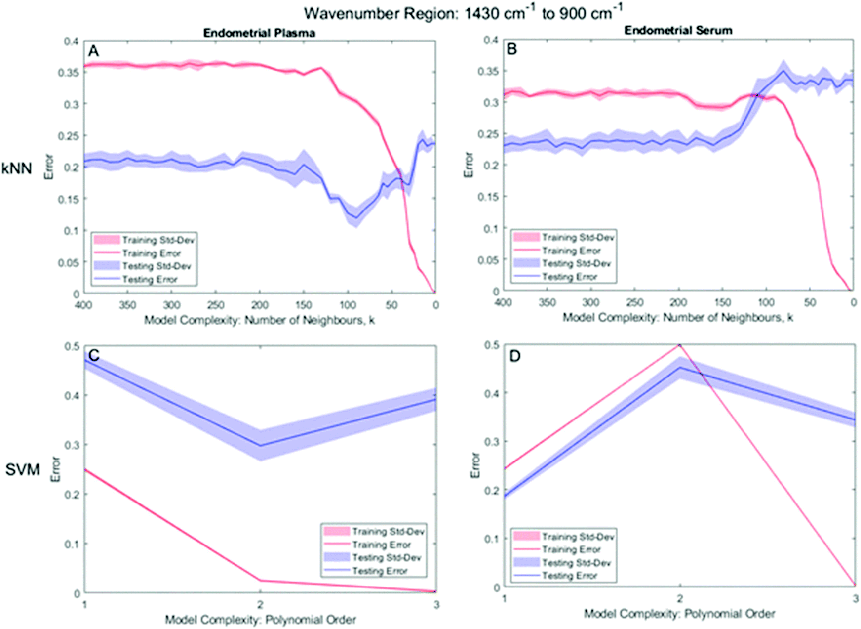 | ||
| Fig. 4 Kernel parameter selection of k for kNN (on the (A) plasma and (B) serum datasets) and the polynomial order for SVM (for the (C) plasma and (D) serum datasets) in the 1430 cm−1 to 900 cm−1 range. | ||
| Endometrial plasma | Endometrial serum | |||||
|---|---|---|---|---|---|---|
| SENS | SPEC | MR | SENS | SPEC | MR | |
| Wavenumber range: 1430 cm−1–900 cm−1 | ||||||
| LDA | 0.642 ± 0.015 | 0.730 ± 0.002 | 0.312 ± 0.007 | 0.899 ± 0.023 | 0.763 ± 0.048 | 0.173 ± 0.035 |
| QDA | 0.530 ± 0.024 | 0.729 ± 0.016 | 0.365 ± 0.014 | 0.991 ± 0.010 | 0.581 ± 0.016 | 0.225 ± 0.012 |
| kNN | 0.865 ± 0.043 | 0.895 ± 0.023 | 0.119 ± 0.017 | 0.703 ± 0.011 | 0.838 ± 0.021 | 0.226 ± 0.014 |
| SVM | 0.737 ± 0.025 | 0.653 ± 0.033 | 0.297 ± 0.065 | 0.919 ± 0.026 | 0.716 ± 0.015 | 0.186 ± 0.007 |
| Wavenumber range: 1800 cm−1–900 cm−1 | ||||||
| LDA | 0.881 ± 0.026 | 0.853 ± 0.030 | 0.134 ± 0.023 | 0.777 ± 0.006 | 0.704 ± 0.003 | 0.262 ± 0.002 |
| QDA | 0.917 ± 0.014 | 0.799 ± 0.007 | 0.145 ± 0.007 | 0.852 ± 0.023 | 0.700 ± 0.162 | 0.228 ± 0.074 |
| kNN | 0.879 ± 0.033 | 0.896 ± 0.024 | 0.112 ± 0.023 | 0.759 ± 0.004 | 0.732 ± 0.012 | 0.255 ± 0.049 |
| SVM | 0.993 ± 0.010 | 0.815 ± 0.000 | 0.110 ± 0.013 | 0.782 ± 0.006 | 0.703 ± 0.004 | 0.260 ± 0.001 |
For the bio-fingerprint region: 1800 cm−1 to 900 cm−1, the number of neighbours, k, which leads to the proper operation condition of the kNN classifier is k = 180 and k = 60 for the plasma and serum sample, respectively, while a PO of 1 of SVM for both plasma and serum sample. For kNN, Fig. 5A and B shows that the minima for the MR for kNN classification of testing datasets occurs at k = 180 (MR = 0.112 ± 0.023) for the plasma sample and at k = 60, (MR of 0.255 ± 0.049) for the serum sample. For SVM, Fig. 5C and D shows that SVM with PO = 1 leads to the minima for the MR for both the plasma (MR = 0.110 ± 0.013) and serum (MR = 0.260 ± 0.001) sample (Table 2).
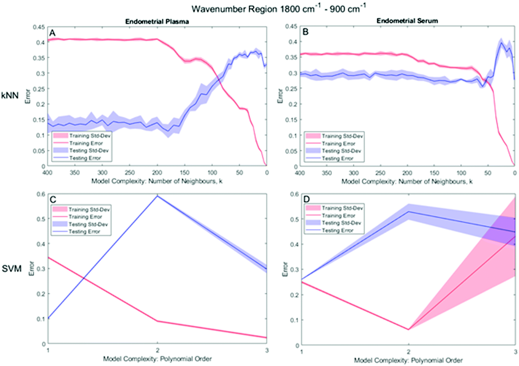 | ||
| Fig. 5 Kernel parameter selection of k for kNN (on the (A) plasma and (B) serum datasets) and the polynomial order for SVM (for the (C) plasma and (D) serum datasets) in the 1800 cm−1 to 900 cm−1 range. | ||
3.2. Classifier performance
Fig. 6 depicts the MCC metric for the discrimination of MIR spectral data from the wavenumber regions of 1430 cm−1 to 900 cm−1 and 1800 cm−1 to 900 cm−1 performed by the LDA, QDA, kNN and SVM classifiers.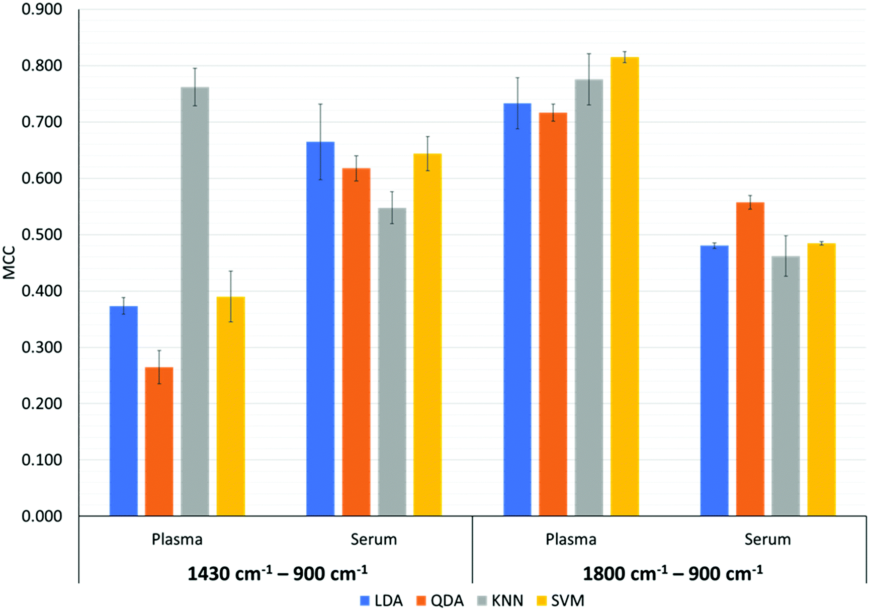 | ||
| Fig. 6 Classification performance of each model in the 1430 cm−1 to 900 cm−1 and 1800 cm−1 to 900 cm−1 range for plasma and serum. This metric ranges from −1 to +1, where an MCC of 1 indicates a perfect classifier, an MCC of −1 indicates a classifier that misclassifies all classes and an MCC of 0 indicates a classifier that classifies at an accuracy equivalent to the flip of a coin. | ||
For the bio-fingerprint region: 1430 cm−1 to 900 cm−1, Fig. 6 shows that in general the discrimination task based on the serum samples produces higher value for the MCC metric compared to when discrimination is performed on the plasma samples, except when the kNN classifier is used. In detail, the MCC for the discrimination of the serum testing datasets using LDA, QDA and SVM (PO = 1) are 0.664 ± 0.067, 0.618 ± 0.022 and 0.644 ± 0.030, respectively. However, for the plasma datasets, the MCC for LDA, QDA and SVM (PO = 2) are 0.373 ± 0.015, 0.265 ± 0.029 and 0.390 ± 0.045, respectively. For the kNN classifier, an MCC of 0.762 ± 0.034 and 0.548 ± 0.028 are produced for discrimination based on plasma and serum testing datasets, respectively. Noting that the k-parameter of the kNN classifier is k = 90 when discriminating the plasma dataset and k = 310 when discriminating the serum dataset. The corresponding sensitivity and specificity of the kNN with the highest MCC (k = 90) are 0.865 ± 0.043 and 0.895 ± 0.023, respectively.
For the bio-fingerprint region 1800 cm−1 to 900 cm−1, Fig. 6 shows that a higher MCC metric is observed when the discrimination is performed on the plasma datasets than when the discrimination is performed on the serum datasets regardless of the classifier used. In detail, the MCC for the discrimination based on the plasma datasets are 0.733 ± 0.046, 0.717 ± 0.015, 0.776 ± 0.045 and 0.815 ± 0.010 for LDA, QDA, kNN and SVM, respectively. For the serum datasets, the MCC are 0.481 ± 0.005, 0.557 ± 0.012, 0.490 ± 0.011 and 0.485 ± 0.003 for LDA, QDA, kNN and SVM, respectively. The corresponding sensitivity and specificity of the SVM with the highest MCC are 0.993 ± 0.010 and 0.815 ± 0.000, respectively. The performance of each classifier for all the plasma and serum datasets is presented in Table 2.
3.3. Important features
Here, the important features (i.e., spectral wavenumbers) based on the MIR spectroscopy of plasma and serum samples are analysed based on the framework described in section 2.3.4 [see Fig. S3 and S4 of ESI†].For the bio-fingerprint region: 1430 cm−1 to 900 cm−1, important features shared by both plasma and serum datasets are at 1358 cm−1 (CO stretching of –COO–), 1346 cm−1 to 1288 cm−1 (C–N/N–H deformation of Amide III), 1215 cm−1 to 1254 cm−1 (asym PO stretching in PO2− in DNA), 1192 cm−1 to 1165 cm−1 (sym C–O–C and C–O–P stretching and ring vibrations, sym C–O stretching coupled with C–O–H bending), 1092 cm−1 to 1088 cm−1 (sym stretching in PO2− and CO–O–C sym stretching in DNA) and 999 cm−1 (sym C–O stretching). Unique important features found in the plasma dataset are at 1360 cm−1 and 1038 cm−1, accounting for C–N stretching in tyrosine and guanine, and sym stretching of C–O–C, respectively. Unique features found in serum and not in plasma dataset are 1423 cm−1, 1393 cm−1 and 937 cm−1, accounting for the stretching of CO of –COO–, the sym C–H deformation of CH3 and the stretching of C–O/C–C, respectively23 (see Table S1†).
For the bio-fingerprint region 1800 cm−1 to 900 cm−1, important features, unique to this wavelength region, found in both datasets (plasma and serum) are at 1778 cm−1 to 1720 cm−1 (CO stretching of esters), 1690 cm−1 to 1670 cm−1 (from secondary protein conformations: anti-parallel β sheets, loops and turns), 1643 cm−1 to 1601 cm−1 (CO stretching of Amide I, assigned to glycoproteins such as fibrinogen) and 1570 cm−1 to 1508 cm−1 (N–H bending, C–H stretching, C–O bending, C–C and N–C stretching of Amide II also assigned to glycoproteins such as fibrinogen). Important features unique to serum are at 1467 cm−1 to 1450 cm−1 (sym and asym C–H scissoring of –CH3), 1161 cm−1, and 1099 cm−1.23,44 No important features unique to plasma dataset found (see Table S2†).
4. Discussion
Herein, we have demonstrated that plasma and serum-based MIR spectroscopy paired with an optimised classifier, have the capability to discriminate between endometrial cancers and controls. There is a strong research interest for the collection of MIR spectral data from patients with cancer, in vivo.45–48 A major limiting factor when using MIR spectroscopy in vivo, is the presence of water in tissue. When collecting MIR spectra from hydrated tissue, a strong H–O–H bending vibration at 1610 cm−1 dominates the bio-fingerprint region, and consequently information from the Amide I (1601 cm−1), Amide II (1645 cm−1) and adjacent bands are lost.23 One way to mitigate against this, when classifying in vivo MIR spectral data is to focus on a different part of the MIR spectrum, i.e., a region of the spectrum not influenced by the H–O–H vibration.In this work, we investigated two different pre-processing techniques that differed on the spectral region: the first, a section from the bio-fingerprint region (1430 cm−1 to 900 cm−1) and the second, a more extended bio-fingerprint region (1800 cm−1 to 900 cm−1). Investigating only a section of the bio-fingerprint region allowed us to assess the performance of various classification classifiers in discriminating between cancerous and controls, with less spectral information. We have demonstrated for the first time that even with this limitation (i.e., smaller spectral range of 1430 cm−1 to 900 cm−1) classifiers are able to discriminate between cancerous and control of endometrial plasma and serum samples with high fidelity (achieving a SENS of 0.865 ± 0.043 and SPEC of 0.895 ± 0.023 for kNN with plasma and a SENS of 0.899 ± 0.023 and SPEC of 0.763 ± 0.048 for LDA with serum).
A distinct observation made when considering the performance of each classifier for the two pre-processing techniques is that the classifiers seem to perform considerably better with plasma in the 1800 cm−1 to 900 cm−1 range than in the 1430 cm−1 to 900 cm−1 range, while the opposite is true for serum (a better performance is observed in the latter range than the former) (Fig. 6 and Table 2). The rationale for this is due to the differences in the content of protein and free DNA in plasma and serum. Plasma and serum essentially have the same composition, 50% to 60% albumins and 40% globulins. The exception is the presence of fibrinogens and clotting factors in plasma, which are absent in serum.49 Further studies into the differences between plasma and serum have shown that, serum has a higher concentration of metabolites50 and circulating free DNA (cfDNA),51,52 which serve as potential biomarkers for disease detection. In the case of plasma, various studies have investigated the use of fibrinogen as a biomarker for endometrial cancer.53–55
Our analysis suggests that the reason for the better classifier performance for plasma in the 1800 cm−1 to 900 cm−1 range, is due to the presence of IR signals (Amide I and Amide II) attributed to fibrinogen. This is supported by work by Seebacher et al.,53 and Zhou et al.,55 which reported significant increased levels of fibrinogen, associated with patients with endometrial cancer, at advanced stages. Interestingly, as seen in Fig. 6, for plasma, the performance of kNN is not affected by the spectral region being investigated. This is believed to be due to the different working principle of kNN compared to the other classifiers considered in the present work. That is, that LDA, QDA and SVM classify by drawing a (hyper)plane between two or more classes that best describes the differences between the classes.24,31 kNN, however, classifies unknown observation based on a majority vote of their neighbours, with each observation being assigned to the class most common among its k nearest neighbours.24 Therefore, if there are well-defined clusters in the dataset, an optimised kNN classifier is likely to perform well. This was the case in our work, where, after PCA, defined clusters were formed when each PC was compared (see Fig. S5†). In regard to serum, we believe that the main difference between cancer and control, is the presence of increased levels of cfDNA, as discussed in.56,57 Our results suggest that the inclusion of the Amide I and Amide II regions, dilutes the importance of the cfDNA IR signals. The consequence of this is a reduced performance from each classifier in the 1800 cm−1 to 900 cm−1 region.
There are two factors that determine how well a classifier will perform: its ability to achieve a small training and testing error and its ability to minimise the gap between the training and testing errors. These factors correspond to the proper selection of kernel parameters for ML-based classifiers, to avoid over-fitting and under-fitting.43 Over-fitting occurs when a classifier learns the intricate details of the training data thus negatively impacting its performance on unseen data, whereas under-fitting refers to a classifier that is unable to classify the training data (resulting in a high training error) nor generalise to new data (resulting in a high testing error) due to the lack of kernel's dimensionality.43 Of the two, it is more difficult to detect over-fitting and reduce the risk of this happening (depending on the analyst skills).24 Data decomposition using feature extraction methods, such as PCA, partial least squares (PLS), FFS and iterative feature selection, is one way to reduce the risk of over-fitting.31 The implementation of such methods is particularly important when considering vibrational spectroscopy-based data, due to their high dimensional nature. For example, applying PCA to the plasma dataset (1430 cm−1 to 900 cm−1) in this work, reduced the number of dimensions in the dataset from 137 wavenumbers to 9 PCs, accounting for 95% variance in the dataset (see Fig. S5–S8†). This, however, is not always sufficient, especially when implementing non-parametric algorithms (such as kNN and SVM) with multiple complexity parameters that each require optimising.24 For instance, with SVM there are multiple kernel functions that could be selected (linear, polynomial or radial-basis-function (RBF)), within which exists even more kernel parameters that should be assessed during optimisation (e.g., the polynomial order for the polynomial kernel).41 Similarly, with kNN, which although is not as complex as SVM, still requires optimisation at multiple levels (i.e., the distance weighting function (equal, inverse, or squared inverse), followed by k, the number of neighbours).24 In this work, we found that the most ideal distance weighting function for kNN was the equal weight, as opposed to the inverse or squared inverse function, which both resulted in consistently overfit classifiers with our datasets (results not shown). Regarding SVM, the polynomial order kernel was selected as it is known to be less susceptible to over-fitting when compared to the RBF kernel, but more capable of modelling complex data patterns as opposed to the linear kernel. In our work, the framework used to obtain the optimum classifier complexity and so further minimise the risk of over-fitting, as described in section 2.3.3. Is discussed in detail by Goodfellow et al.43
5. Conclusions
We have demonstrated that, even when a portion of the bio-fingerprint region has been removed (leaving only 1430 cm−1 to 900 cm−1), the MIR spectroscopy of dried blood plasma bio-fluids can be used to discriminate endometrial cancer from controls, with high fidelity (MCC: 0.762 ± 0.034, SENS: 0.865 ± 0.043, SPEC: 0.865 ± 0.023) when paired with the kNN classifier. This shows that there is potential behind the use of the 1430 cm−1 to 900 cm−1 region of the bio-fingerprint for the classification of endometrial cancer. These findings further suggest the potential inclusion of MIR spectroscopy as screening tool for endometrial cancer in vivo and ex vivo in clinical practice.Ethics statement
All patients gave written informed consent before any protocol-specific procedure was performed. The samples were from patients undergoing gynaecological surgery in the Royal Preston Hospital of Lancashire Teaching Hospitals NHS Foundation Trust in Preston between January 2006 and August 2012. Ethical committee approvals were obtained (Local Research Ethical Committee (LREC) approval no. 05/Q1302/83 and the Research and Ethics Committee (REC) approval no. 10/H0308/75). The consenting patients were between the ages of 37 and 90 years. All experiments were conducted according to the principles of the Declaration of Helsinki and all other applicable national or local laws and regulations.Funding
This work was supported by the Engineering and Physical Sciences Research Council (EPSRC) [via grant number EP/N50970X/1 and through the thematic programme: Wave Phenomena in Complex Media and EP/M008983/1].Conflicts of interest
F. L. M. is a shareholder in Biocel UK Ltd, a company looking to develop spectroscopy tools and analytical techniques for diagnostic/screening purposes.References
- P. Buderath, P. Rusch, P. mach and R. Kimmig, Cancer field surgery in endometrial cancer: peritoneal mesometrial resection and targeted compartmental lymphadenectomy for locoregional control, J. Gynecol. Oncol., 2021, 32(1), 1–12 CrossRef PubMed.
- P. A. Sanderson, A. Moulla and S. K. Fegan, Endometrial cancer - an update, Obstet. Gynaecol. Reprod. Med., 2019, 29(8), 225–232 CrossRef.
- F. Bray, J. Ferlay, I. Soerjomataram, R. L. Siegel, L. A. Torre and A. Jemal, Global cancer statistics 2018: GLOBOCAN estimates of incidence and mortality worldwide for 36 cancers in 185 countries, Ca–Cancer J. Clin., 2018, 68(6), 394–424 CrossRef PubMed.
- GLOBOCAN 2. Corpus uteri., 2020.
- V. Masciullo, G. Amadio, D. L. Russo, I. Raimondo, A. Giordano and G. Scambia, Controversies in the management of endometrial cancer, Obstet. Gynecol. Int., 2010, 2010 Search PubMed.
- S. Walker, C. Hyde and W. Hamilton, Risk of uterine cancer in symptomatic women in primary care: case–control study using electronic records, Br. J. Gen. Pract., 2013, 63(614), e643–e648 CrossRef PubMed.
- R. D. Langer, J. J. Pierce, K. A. O'Hanlan, S. R. Johnson, M. A. Espeland and J. F. Trabal, et al., Transvaginal ultrasonography compared with endometrial biopsy for the detection of endometrial disease, N. Engl. J. Med., 1997, 337, 1792–1798 CrossRef CAS PubMed.
- A. Gentry-Maharaj and C. Karpinskyj, Current and future approaches to screening for endometrial cancer, Best Pract. Res. Clin. Obstet. Gynaecol., 2020, 65, 79–97 CrossRef CAS PubMed.
- U. Menon, A. Gentry-Maharaj, R. Hallett, A. Ryan, M. Burnell and A. Sharma, et al., Sensitivity and specificity of multimodal and ultrasound screening for ovarian cancer, and stage distribution of detected cancers: results of the prevalence screen of the UK Collaborative Trial of Ovarian Cancer Screening (UKCTOCS), Lancet Oncol., 2009, 10(4), 327–340 CrossRef.
- I. Jacobs, A. Gentry-Maharaj, M. Burnell, R. Manchanda, N. Singh and A. Sharma, et al., Sensitivity of transvaginal ultrasound screening for endometrial cancer in postmenopausal women: a case-control study within the UKCTOCS cohort, Lancet Oncol., 2011, 12(1), 38–48 CrossRef PubMed.
- A. Sala, D. J. Anderson, P. M. Brennan, H. J. Butler, J. M. Cameron and M. D. Jenkinson, et al., Biofluid diagnostics by FTIR spectroscopy: A platform technology for cancer detection, Cancer Lett., 2020, 477, 122–130 CrossRef CAS PubMed.
- D. Sheng, X. Liu, W. Li, Y. Wang, X. Chen and X. Wang, Distinction of leukemia patients’ and healthy persons’ serum using FTIR spectroscopy, Spectrochim. Acta, Part A, 2013, 101, 228–232 CrossRef CAS PubMed.
- D. Sheng, Y. Wu, X. Wang, D. Huang, X. Chen and X. Liu, Comparison of serum from gastric cancer patients and from healthy persons using FTIR spectroscopy, Spectrochim. Acta, Part A, 2013, 116, 365–369 CrossRef CAS PubMed.
- I. Van der Auwera, H. J. Elst, S. J. Van Laere, H. Maes, P. Huget and P. Van Dam, et al., The presence of circulating total DNA and methylated genes isassociated with circulating tumour cells in blood from breastcancer patients, Br. J. Cancer, 2009, 100, 1277–1286 CrossRef CAS.
- J. J. Choi, C. F. Reich III and D. S. Pisetsky, Release of DNA from Dead and Dying Lymphocyte and Monocyte Cell Lines In Vitro, Scand. J. Immunol., 2004, 60(1–2), 159–166 CrossRef CAS PubMed.
- L. Keller, Y. Belloum, H. Wikman and K. Pantel, Clinical relevance of blood-based ctDNA analysis: mutation detection and beyond, Br. J. Cancer, 2021, 124, 345–358 CrossRef.
- K. Gajjar, J. Trevian, G. Owens, P. J. Keating, N. J. Wood and H. F. Stringfellow, et al., Fourier-transform infrared spectroscopy coupled with a classification machine for the analysis of blood plasma or serum: a novel diagnostic approach for ovarian cancer, RSC Analyst, 2013, 138, 3917–3926 RSC.
- A. M. Gilbey, D. Burnett, R. E. Coleman and I. Holen, The detection of circulating breask cancer cells in blood, J. Clin. Pathol., 2004, 57(9), 903–991 CrossRef CAS PubMed.
- BS-EN-ISO., Optics and photonics. Spectral bands. (BS ISO20473:2007), 2007.
- K. Su and W. Lee, Fourier transform infrared spectroscopy as a cancer screening and diagnostic tool: a review and prospects, Cancers, 2020, 12(1), 1–19 CrossRef PubMed.
- V. Balan, C. Mihai, F. Cojocaru, C. Uritu, G. Dodi and D. Botezat, et al., Vibrational spectroscopy fingerprinting in medicine: from molecular to clinical practice, Materials, 2019, 12(18), 1–40 CrossRef PubMed.
- E. Kontsek, A. Pesti, M. Bjornstedt, T. Uveges, E. Szabo and T. Garay, et al., Mid-infrared imaging is able to characterize and separate cancer cell lines, Pathol. Oncol. Res., 2020, 26, 2401–2407 CrossRef CAS PubMed.
- L. Shi and R. Alfano, Deep imaging in tissue and biomedical materials, Pan Stanford Publishing, 2017 Search PubMed.
- C. L. M. Morais, K. M. G. Lima, M. Singh and F. L. Martin, Tutorial: multivariate classification for vibrational spectroscopy in biological samples, Nat. Protoc., 2020, 15, 21 Search PubMed.
- J. Luo, K. Ying and J. Bai, Savitzky–Golay smoothing and differentiation filter for even number data, Signal Process., 2005, 85(7), 1429–1434 CrossRef.
- B. K. Alsberg, A. M. Woodward, M. K. Winson, J. Rowland and D. B. Kell, Wavelet denoising of infrared spectra, Analyst, 1997, 122, 645–562 RSC.
- G. Luo, G. Chen, L. Tian and S. Qian, Minimum noise fraction verses principle component analysis as a preprocessing step for hyperspectral imagery denoising, Can. J. Remote Sens., 2016, 42, 106–116 CrossRef.
- B. Mohlenhoff, M. Romeo, M. Diem and B. R. Wood, Mie-type scattering and non-Beer-Lambert absorption behavior of human cells in infrared microspectroscopy, Biophys. J., 2005, 88(5), 3635–3640 CrossRef CAS PubMed.
- P. Bassan, H. J. Bryne, F. Bonnier, J. Lee, P. Dumasc and P. Gardner, Resonant Mie scattering in infrared spectroscopy of biological materials - understanding the ‘dispersion artefact’, Analyst, 2009, 134, 1586–1593 RSC.
- A. Kohler, J. Sule-Suso, G. D. Sockalingum, M. Tobin, F. Bahrami and Y. Yang, et al., Estimating and correcting Mie scattering in synchotron-based microscopuc fourier transform infrared spectra by extended muliplicative signal correction, Appl. Spectrosc., 2008, 62(3), 259–266 CrossRef CAS.
- M. J. Baker, J. Trevisan, P. Bassan, R. Bhargava, H. J. Butler and K. M. Dorling, et al., Using fourier transform IR spectroscopy to analyze biological materials, Nat. Protoc., 2014, 9(8), 1771–1791 CrossRef CAS.
- S. Suthaharan, Machine learning models and algorithms for big data classification, Springer, New York, 2016 Search PubMed.
- J. Backhaus, R. Mueller, N. Formanski, N. Szlama, H. Meerpohl and M. Eidt, et al., Diagnosis of breast cancer with infrared spectroscopy from serum samples, Vib. Spectrosc., 2010, 52, 173–177 CrossRef CAS.
- J. Ollesch, S. L. Drees, H. M. Heise, T. Behrens, T. Bruning and K. Gerwert, FTIR spectroscopy of biofluids revisited: an automated approach to spectral biomarker identification, Analyst, 2013, 138(14), 4092–4102 RSC.
- A. Sala, D. J. Anderson, P. M. Brennan, H. J. Butler, J. M. Cameron and M. D. Jenkinson, et al., Biofluid diagnostics by FTIR spectroscopy: A platform technology for cancer detection, Cancer Lett., 2020, 477, 122–130 CrossRef CAS.
- I. Maitra, C. L. M. Morais, K. M. G. Lima, K. M. Ashton, R. S. Date and F. L. Martin, Attenuated total reflection Fourier-transform infrared spectral discrimination in human bodily fluids of oesophageal transformation to adenocarcinoma, RSC Analyst, 2019, 144, 7447–7456 RSC.
- P. P. Angelov and X. Zhou, Evolving Fuzzy-rule-based classifiers from data streams, IEEE Trans. Fuzzy Syst., 2008, 16(6), 1462–1475 Search PubMed.
- A. J. Izenman, Modern multivariate statistical techniques, Springer, 2008 Search PubMed.
- A. Tharwat, Linear vs. quadratic discriminant analysis classifier: a tutorial, Int. J. Appl. Pattern Recognit., 2016, 3(2), 145–180 CrossRef.
- G. Guo, H. Wang, D. Bell, Y. Bi and K. Greer, KNN model-based approach in classification, in On the move to meaningful internet systems 2003: CoopIS, DOA, and ODBASE. OTM 2003. Lecture notes in computer science, Springer Berlin Heidelberg, Berlin, Heidelberg, 2003, p. 986–996 Search PubMed.
- N. Cristianini and J. Shawe-Taylor, An introduction to support vector machines and other kernel-based learning methods, Cambridge University Press, Cambridge, 2014 Search PubMed.
- D. Chicco and G. Jurman, The advantages of the Matthews correlation coefficient (MCC) over F1 score and accuracy in binary classification evaluation, BMC Genomics, 2020, 21(6), 1–13 Search PubMed.
- I. Goodfellow, Y. Bengio and A. Courville, Deep Learning Cambridge, The MIT Press, Massachusetts, 2016 Search PubMed.
- M. Boix, S. Eslava, G. C. Machado, E. Gosselin, N. Ni and E. Saiz, et al., ATR-FTIR measurements of albumin and fibrinogen adsorption: Inert verses calcium phosphate ceramics, J. Biomed. Mater. Res., Part A, 2015, 103(11), 3493–3502 CrossRef CAS.
- A. B. Seddon, B. Napier, I. Lindsay, S. Lamrini, P. M. Moselund and N. Stone, et al., Mid-infrared spectroscopy/bioimaging: moving toward MIR optical biopsy, Laser Focus World., 2016, 52(2), 50–53 CAS.
- A. B. Seddon, B. Napier, I. Lindsay, S. Lamrini, P. M. Moselund and N. Stone, et al., Prospective on using fibre mid-infrared supercontinuum laser sources for in vivo spectral discrimination of disease, Analyst, 2018, 143(24), 5874–5887 RSC.
- Q. Li, Z. Xu, N. Zhang, L. Zhang, F. Wang and L. Yang, et al., In vivo and in situ detection of colorectal cancer using Fourier transform infrared spectroscopy, World J. Gastroenterol., 2005, 11(3), 327–330 CrossRef CAS PubMed.
- L. Dong, X. Sun, Z. Chao, S. Zhang, J. Zheng and R. Gurung, et al., Evaluation of FTIR spectroscopy as diagnostic tool for colorectal cancerusing spectral analysis, Spectrochim. Acta, Part A, 2013, 122, 288–294 CrossRef.
- M. Leeman, J. Choi, S. Hansson, M. U. Storm and L. Nilsson, Proteins and antibodies in serum, plasma, and whole blood—size characterization using asymmetrical flow field-flow fractionation (AF4), Anal. Bioanal. Chem., 2018, 410(20), 4867–4873 CrossRef CAS PubMed.
- Z. Yu, G. Kastenmuller, Y. He, P. Belcredi, G. Moller and C. Prehn, et al., Differences between human plasma and serum metabolite profiles, PLoS One, 2011, 6(7), 1–6 Search PubMed.
- A. Zinkova, I. Brynychova, A. Svacina, M. Jirkovska and M. Korabecna, Cell-free DNA from human plasma and serum differs in content of telomeric sequences and its ability to promote immune response, Sci. Rep., 2017, 7(2591), 1–8 CAS.
- T. Lee, L. Montalvo, V. Chrebtow and M. P. Busch, Quantitation of genomic DNA in plasma and serum samples: higher concentrations of genomic DNA found in serum than in plasma, Transfusion., 2001, 41, 276–282 CrossRef CAS PubMed.
- V. Seebacher, S. Polterauer, C. Grimm, H. Husslein, H. Leipold and K. Hefler-Frischmuth, et al., The prognostic value of plasma fibrinogen levels in patients with endometrial cancer: a multi-centre trial, Br. J. Cancer, 2010, 102, 952–956 CrossRef CAS PubMed.
- Q. Li, R. Cong, F. Kong, J. Ma, Q. Wu and X. Ma, Fibrinogen is a coagulation marker association with the prognosis of endometrial cancer, OncoTargets Ther., 2019, 12, 9947–9956 CrossRef CAS.
- X. Zhou, H. Wang and X. Wang, Preoperative CA125 and fibrinogen in patients with endometrial cancer: a risk model for predicting lymphovascular space invasion, J. Gynecol. Oncol., 2017, 28(2), 1–11 Search PubMed.
- L. Cicchillitti, G. Corrado, M. D. Angeli, E. Mancini, E. Baiocco and L. Patrizi, et al., Circulating cell-free DNA content as blood based biomarker in endometrial cancer, Oncotarget, 2017, 8(70), 115230–115243 CrossRef.
- E. Vizza, G. Corrado, M. D. Angeli, M. Carosi, E. Mancini and E. Baiocco, et al., Serum DNA integrity index as a potential molecular biomarker in endometrial cancer, J. Exp. Clin. Cancer Res., 2018, 37(16) CAS.
Footnote |
| † Electronic supplementary information (ESI) available. See DOI: 10.1039/d1an00833a |
| This journal is © The Royal Society of Chemistry 2021 |