
 Open Access Article
 This Open Access Article is licensed under a Creative Commons Attribution-Non Commercial 3.0 Unported Licence
Development of a numerical simulation method for modelling column breakthrough from extraction chromatography resins
Frances M.
Burrell
 *a,
Phillip E.
Warwick
a,
Ian W.
Croudace
b and
W. Stephen
Walters
c
*a,
Phillip E.
Warwick
a,
Ian W.
Croudace
b and
W. Stephen
Walters
c
aGAU-Radioanalytical, University of Southampton, European Way, Southampton SO14 3ZH, UK. E-mail: Frances.Burrell@noc.soton.ac.uk
bUniversity of Southampton, European Way, Southampton SO14 3ZH, UK
cReactor Materials and Chemistry, National Nuclear Laboratory Limited, NNL Culham, Building D5, First Floor, Culham Science Centre, Abingdon, Oxfordshire OX14 3DB, UK
First published on 25th May 2021
Abstract
A numerical simulation method has been developed to describe the transfer of analytes between solid and aqueous phases and assessed for a commercially available extraction chromatography resin (UTEVA resin). The method employs an ordinary differential equation solver within the LabVIEW visual programming language. The method was initially developed to describe a closed batch system. The differential equations and kinetic rate constants determined under these conditions were then applied to the flow-through column geometry. This was achieved by modelling the resin bed as a series of discrete vertically stacked sections, thereby generating an array of solid and aqueous concentration values. Axial flow was simulated by the advancement of the aqueous phase values by one array position with the value advancing from the final array position representing the column output concentration. An investigation into the observed difference in breakthrough profiles obtained under repeated conditions revealed the relative tolerance of the numerical simulation method to errors in each input parameter. Additional physical processes such as backpressure and leaching of the extractant were considered as an explanation for observed inconsistencies between experimental and simulated datasets. An elution sequence featuring multiple eluents was also simulated, demonstrating that the prediction of analyte separation sequences is possible. The potential to develop the LabVIEW coding into user friendly software with an extendable kinetic database is also discussed. This software will be a useful tool to radiochemists particularly in the development of new analytical methods using automated separation systems.
1. Introduction
Implementation of efficient and robust radioanalytical separation schemes is necessary to underpin nuclear operations, radioactive waste characterisation, nuclear forensics, and environmental monitoring programmes. Development and optimisation of radioanalytical separation schemes can be an extensive process even if experimental optimisation techniques are followed; this process is complicated if vacuum box or pump technology is used to enhance the flow rate through the column. A software tool capable of simulating elution profiles under a range of flow rates, bed dimensions, sample volumes and matrices would therefore facilitate efficient method development. In addition, optimising column operating parameters for each sample matrix to reduce analysis time, improve separation factors and minimise waste and reagent consumption could increase the efficiency of routine analysis.Mathematical equations can be used to describe the movement of dissolved species in a packed bed. These equations often describe the concentration change with respect to time and can be solved to predict the concentration either on the column or in the column output solution at any given time. Depending on the complexity of the equations chosen and any assumptions made, the solution can be obtained using either algebraic or numerical methods.1,2 Numerical solution involves iterative adjustment of concentrations at either set or variable time steps until all equations are met to a defined level of accuracy across the specified time period.
The most complete approach to chromatographic simulation is known as the general rate model. This approach employs a series of partial differential equations describing concentration change in terms of both time and position distinguishing between the aqueous and solid phases (pore concentration and sorbed concentration), axial distribution on the column and radial distribution within the solid particles. Concentration change can occur via any of the four main chromatographic processes:3–6 (1) fluid flow and aqueous phase dispersion; (2) diffusion across the stagnant layer surrounding the solid particles (film diffusion); (3) diffusion within the sorptive material (intraparticle diffusion); and (4) the chemical reaction (e.g. ion exchange or complexation). Due to its complexity, the general rate model can only be solved using a computational partial differential equation solver. Simplifications can be applied to reduce the description of chromatographic processes to a series of ordinary differential equations.
The system can be further simplified by representing a chromatographic column as a set of axially distributed closed systems (Fig. 1). Within each closed system, species may transfer between the two phases in an attempt to reach equilibrium. Unlike a closed system, however, the aqueous phase is mobile, meaning that the concentration in contact with the stationary solid phase can change. As a consequence, the probability of a molecule in the solid phase to either remain or transfer back into the aqueous phase can also change.
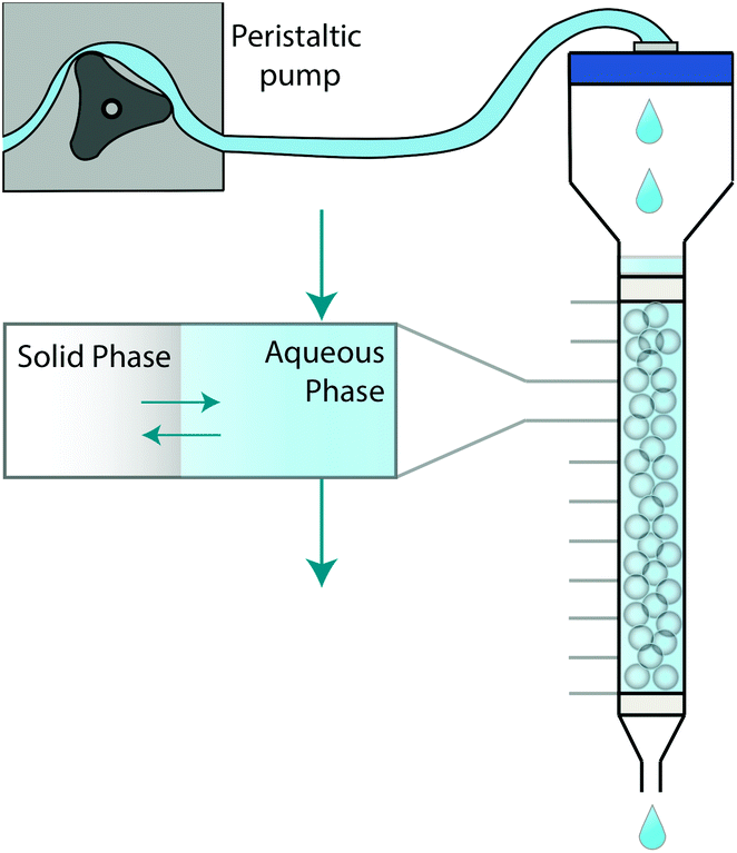 | ||
| Fig. 1 Graphical depiction of numerical simulation method for chromatographic breakthrough. Note: Not to scale. | ||
This paper proposes a method based on the development of differential equations to describe the kinetics and thermodynamics of batch sorption/desorption and the subsequent application of these equations to flow-through column geometry. The method has been demonstrated and validated using a radioanalytical extraction chromatography resin (UTEVA resin). Analyte transfer between the solid and aqueous phases was simulated within each axial division to produce an array of solid and aqueous concentration values; this was followed by advancement of the aqueous phase values by one array position. The duration of time to simulate analyte transfer between the two phases is directly calculated from the flow rate. This process was repeated with the aqueous concentration value in the final array position generating the simulation of column output.
Extraction chromatography resins are commonly used to separate analytes from aqueous or dissolved samples. In this real-life scenario, both interacting and non-interacting species will be present alongside the analyte being isolated. Depending on their concentration and speciation, interferents can have various effects including synergistic sorption, competitive sorption or competitive complex formation.7,8
Several free (PHREEQC, Orchestra, CHEAQS) or licensed (COMSOL Multiphysics, MATLAB, The Geochemist's Workbench, gPROMS) software packages are capable of simulating the kinetics of batch sorption. Simulation control can vary from constrained input of constants and initial conditions to a blank coding environment in which the user can specify all conditions and processes using a glossary of programmed keywords. The former may lack the flexibility to account for both sorption and mass transfer processes or accurately describe complex relationships between sorptive materials and solutions containing multiple analytes.
An alternative approach to coding is offered by National Instruments LabVIEW; this software provides a blank coding environment where conditions and processes are added by inserting, positioning and connecting graphically represented structures and functions. Although LabVIEW is most commonly used in the control of hardware and acquisition of data, the extensive data manipulation capability makes it a suitable option for kinetic simulation.
Column breakthrough is a more complex system to simulate than batch sorption/desorption due to the increased input parameters and uncertainties in their definition. Inaccurate input or over simplification of one of the input parameters may have a significant impact on the breakthrough simulation. Combined parameter errors may also have either an additive or opposing effect depending on the operating conditions; it is therefore difficult to isolate input errors. In addition, the rate of movement of a species down a column is not only determined by interaction with the solid phase but by molecular diffusion within the aqueous phase and the velocity range of the solution due to different paths through the packed bed. The combination of the last two factors is known as axial dispersion and is dependent on the molecular diffusivity of the species, the column packing density, the linear flow velocity and the particle size.2,9,10
In this study, the relationship between the two axial dispersion processes was estimated from breakthrough profiles observed at slow flow rates under which conditions the kinetics of analyte transfer between the two phases has a lesser effect on the shape of breakthrough peaks and the hydrodynamic processes of eddy dispersion and molecular diffusion become more important. The relationship of these three parameters with flow rate has been described by height equivalent of a theoretical plate (HETP) theory using the Van Deemter equation (eqn (1)).
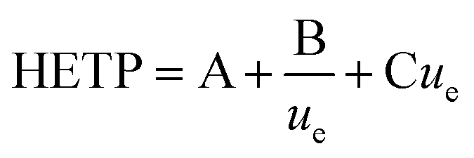 | (1) |
The three terms that make up the HETP value are: eddy dispersion (A) which is independent of aqueous phase velocity; molecular diffusion (B/ue) which is inversely proportional to aqueous phase velocity; and the kinetics of interaction with the solid phase (Cue) which is proportional to aqueous phase velocity. The three plate terms can be combined to calculate the flow rate at which the column exhibits the lowest HETP. Under these conditions, breakthrough peaks would be narrower and more symmetrical leading to better separation between analytes.
Eddy dispersion refers to the non-linear flow of dissolved species travelling down the column. In a packed bed, the presence of solid particles forces the fluid stream to separate and recombine as it travels downwards.2,9,10 The multiple different paths available are not equal in length meaning that although an average residence time within each axial division can be assumed from the flow rate, column dimensions and packing density, the actual residence time for any given molecule sits in a range which is determined by the fastest and slowest routes through the bed. The axial division length (Lax) is a direct representation of the eddy dispersion term (A) as it describes the range associated with the average aqueous phase velocity. A short axial division length would indicate little difference between the slowest and fastest routes through the packed bed whereas a longer length represents a greater range of paths.
Typical radioanalytical chromatographic separations involve the loading of aqueous or digested samples of various volumes and matrix compositions onto the sorptive material and the subsequent sequential elution of analytes. The numerical simulation method was initially evaluated using experimental breakthrough data relating to the loading of a discrete volume (0.025 mL) containing low analyte concentrations and a single wash solution before being extended to a wider range of elution conditions. Competition between analytes was simulated by including the stoichiometry with the extractant in the LabVIEW coding.
This study concludes with a discussion of the potential to refine the coding to produce a software tool with a graphical user interface and an expandable database of rate constants for any extraction chromatography resin, dissolved species, sample matrix composition, and eluting reagent.
2. Experimental
2.1. Reagents and materials
UTEVA resin (100–150 μm) was supplied by TrisKem International, Bruz, FRANCE. Low concentration uranium (as uranyl nitrate) and thorium (as thorium nitrate) solutions (<1 × 10⁻³ mol L−1) were prepared from 1000 mg L−1 elemental stock solutions (Inorganic Ventures, Virginia, USA). High concentrations of uranium and thorium (1 × 10⁻³ mol L−1–8 × 10⁻² mol L−1) were prepared by dissolution of solid nitrate salts (BDH chemicals, no longer licensed). Acids were prepared from Analar grade concentrated solutions and high purity water (18.2 MΩ) from a Milli-Q2 system (Merck, York, UK). All other reagents were from Fisher Scientific, Loughborough, UK unless otherwise specified.2.2. Instrumentation
Stable uranium and thorium concentration measurements were performed on a Thermo Scientific X-series II quadrupole ICP-MS (Thermo Fisher Scientific, Waltham, MA USA) and an Agilent 8800 triple quadrupole ICP-MS (Agilent, Santa Clara, CA, USA). The aqueous solutions were diluted to ppb level and introduced to the instrument in a 2% HNO3 matrix. Six calibration standards (including a 0 ppb solution) were prepared from single element ICP-MS standards (Inorganic Ventures, Virginia, USA). This set was run prior to each batch of samples spanning the expected concentration range of the samples. All calibration standards and samples were spiked with a mixture of In/Re to give a final concentration of 5 ppb for use as internal standards.2.3. Procedures – batch experiments
For batch sorption studies, a known mass (0.01 g–0.1 g) of UTEVA resin was weighed into a polythene vial (22 mL) and 10 ml of 8 M HNO3, 6 M HCl, or 2% HNO3 containing a known concentration of uranium and thorium (10−8 mol L−1–1 mol L−1) was added, recording the new mass and start time. The mixture was allowed to equilibrate for a set amount of time whilst constantly tumbling on a roller mixer. The solution was then filtered through a PTFE syringe filter (0.45 μm) and the concentration remaining in the aqueous phase was measured.For the batch desorption dataset, 1 g of UTEVA resin was mixed with 100 mL of 8 M HNO3 containing a known concentration of uranium and thorium (∼1 × 10⁻⁶ mol L−1) and left to equilibrate for 24 hours before being vacuum filtered using a 0.45 μm cellulose nitrate membrane filter. The recovered resin was left to air dry before a known mass (0.1 g) was weighed into a polythene vial (22 mL) and 10 mL of 8 M HNO3 was added, recording the new mass and start time as before. The mixture was allowed to equilibrate for a set amount of time on a roller mixer. The solution was then filtered through a PTFE syringe filter (0.45 μm) and the concentration of uranium or thorium released into solution was measured.
2.4. Procedures – column experiments
Fresh chromatographic columns were prepared for each experiment by loading a slurry of UTEVA resin in deionised water into a polypropylene column (0.7 cm ID) on top of the preinstalled glass frit. Once the bed had settled and the excess solution drained, another glass frit was positioned on the top of the resin bed to secure the bed. The column was then preconditioned using 8 M HNO3 at a flow rate of ∼2 mL min−1 for 5 minutes. Although care was taken to avoid the column drying out, trapped air bubbles could sometimes be observed. The flow rate through the column was controlled by either a Masterflex 7550-62 (Cole-Palmer UK, London, UK) or a Minipuls3 (Gilson Scientific UK, Bedfordshire, UK) peristaltic pump with Nalgene tubing (2 mm ID). The tubing was attached to the column by a customised lid using Luer fittings.Introduction of small volumes of loading solutions (25 μL) was achieved by removing the lid and pipetting the solution directly on to the top frit and reconnecting the lid before commencing pumping of the wash solution. Introduction of larger volumes of loading solutions (1 mL+) or continuous loading was achieved by inserting the peristaltic pump tubing input into the loading solution and commencing pumping. Once the container was emptied the tubing was quickly moved into the wash solution producing a small air bubble between the two solutions. Collection of breakthrough/elution fractions was achieved using a 2112 Redirac automated fraction collector (LKB Bromma, no longer licensed) or manually by timed exchange of collection vessels. Vessels were weighed before and after collection of fractions to determine the collected mass and hence flow rate.
2.5. Numerical simulation
Numerical simulation was developed using LabVIEW 2015 (National Instruments UK, Newbury, Berkshire). A modular approach to numerical simulation was taken whereby a basic model simulating the transfer of a single species under batch conditions was developed before further levels of complexity were added.2 The key LabVIEW virtual instrument (VI) function used was the pre-programmed ODE solver VI which can solve sets of ordinary differential equations with respect to time (Fig. 2). A list of simulation parameters (Table 1) including the type of solver, tolerances and time steps were programmatically set and remained unchanged for all simulations.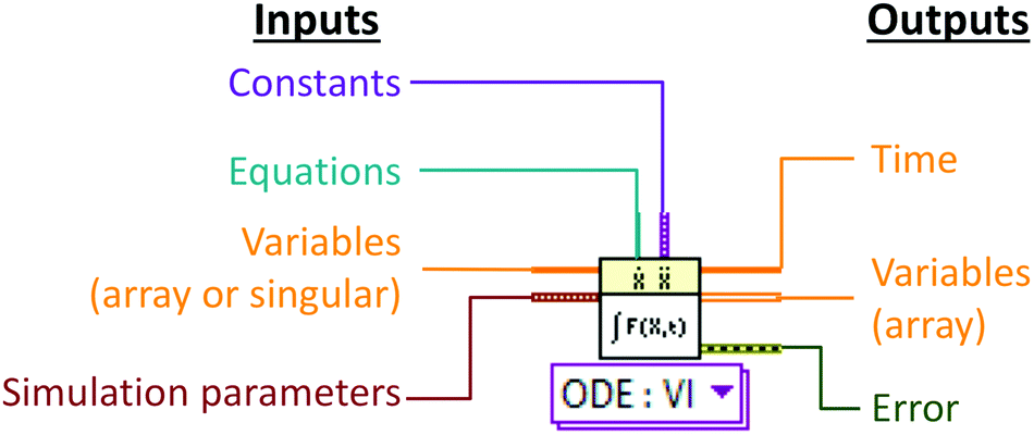 | ||
| Fig. 2 ODE solver as it appears within the LabVIEW graphical development interface. Constants are input as variant data and differential equations are input as a strictly typed reference to the VI that implements the right-hand side of an ordinary differential equation dX/dt = F(X,t). | ||
| Parameter | Value |
|---|---|
| Initial time | 0 |
| Final time | 1 for simulation of batch experiments |
| Variable for simulation of column experiments (see section 2.5.3.) | |
| Time step | 0 (only used if a fixed step-size solver is chosen) |
| Absolute tolerance | 1 × 10⁻⁸ |
| Relative tolerance | 1 × 10⁻⁸ |
| Continuous solver | Runge-Kutta 45 (variable) |
| Discrete time step | Final time/1000 |
| Minimum time step | Final time/1 × 109 |
| Maximum time step | Final time/100 |
| Initial time step | Final time/1000 |
 , a reverse rate constant
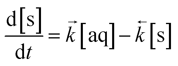
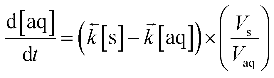
  , the volume fraction of the solid phase (Vs) and the volume fraction of the aqueous phase (Vaq). The variables are singular values for initial analyte concentration in the aqueous phase [aq] and initial analyte concentration in the solid phase [s], following the lumped solid simplification (lumped kinetic model).1,2 For UTEVA resin this lumped solid encompasses the inert polymeric bead and the immobilised organic phase containing the diamyl, amylphosphonate (DAAP) complexant. Unlike other sorptive materials which contain active sites within pores, the numerical simulation method UTEVA resin does not need to consider intraparticle diffusion. The analyte concentration at different locations within the sorptive material and associated internal concentration profiles are not specified; instead the concentration is averaged over the entire volume. The use of constant tumbling conditions also allows for the exclusion of aqueous mass transfer. Both external and internal diffusion could, however, be included for other sorptive materials through modification of the LabVIEW coding (see section 3.7.).
The ODE solver inputs the initial variables and the model constants into two differential equations based on Langmuir kinetics (eqn (2) and (3)) and calculates the temporal change in concentration by solving the two equations simultaneously according to the chosen simulation parameters (Table 1). This generates an array of output variables in the form of analyte concentration in both the solid and aqueous phases along with the corresponding time intervals.
 | (2) |
 | (3) |
As these equations are based on the difference in concentration between two adjacent volumes, the differential equation for the aqueous concentration must include the volumetric ratio of the lumped solid to the aqueous phase in order to achieve mass balance (mol) within the ODE solver VI. In addition, all analyte quantities are converted into mol L−1 prior to input with the mass of solid material converted into a volume by considering the density of the material. This was empirically estimated using a gravimetric liquid displacement technique and determined to be 1.1 g mL−1. This is in agreement with the reference density of UTEVA resin (1.10 g mL−1).11
The final concentration values generated by the ODE solver VI were fed through a while loop shift register to become the ODE solver input variables with the loop iteration value added to the time outputs. A wait of 10 milliseconds was added in order to reduce CPU and memory usage. The stored data was processed and written to a .CSV file using the write delimited spreadsheet VI as well as being displayed on an onscreen XY graph. This graph allows the operator to monitor progress and determine when to stop the simulation.
For simulation of batch sorption, the initial lumped solid analyte concentration was set to zero whereas desorption simulations were initialised with the final lumped solid analyte concentration and an aqueous analyte concentration of zero. Based on the experimental data, the volume of the solid phase was reduced by a factor of 2.7 under desorption conditions. This weight gain could be due to acid retention from the sorption step.
The simulated analyte concentrations in the solid and aqueous phases generated in the .CSV file were combined into a single sorption value taking into account the density (ρ) of the solid for ease of comparison with the experimental data across the range of conditions tested (eqn (4)). Once the system has reached equilibrium this ratio is equivalent to the distribution constant (eqn (5)) which is usually defined as the ratio of analyte concentration on the solid material ([aq]0 − [aq]eq) per solid mass (Ws) to that in the aqueous phase ([aq]eq) per volume (Vaq).
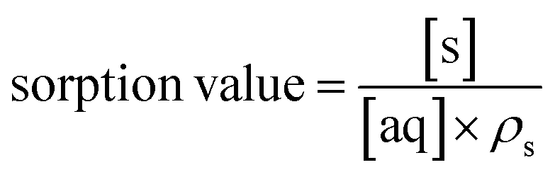 | (4) |
 | (5) |
![[thin space (1/6-em)]](https://www.rsc.org/images/entities/char_2009.gif) :2 stoichiometric reaction with the DAAP extractant11 (eqn (6)) it is therefore proposed that thorium nitrate undergoes a 1:4 stoichiometric reaction with the extractant (eqn (7)); this is a theoretically valid assumption as there are twice as many nitrate ligands surrounding the metal ion.
:2 stoichiometric reaction with the DAAP extractant11 (eqn (6)) it is therefore proposed that thorium nitrate undergoes a 1:4 stoichiometric reaction with the extractant (eqn (7)); this is a theoretically valid assumption as there are twice as many nitrate ligands surrounding the metal ion.| UO2(NO3)2 + 2E ↔ UO2(NO3)2E2 | (6) |
| Th(NO3)4 + 4E ↔ Th(NO3)4E4 | (7) |
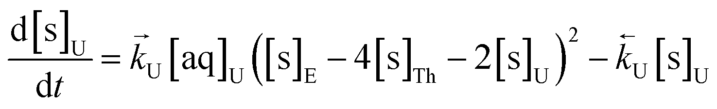
The numerical simulation coding was modified to include a lumped solid extractant concentration model constant ([s]E) as determined via isotherm experiments, rate constants for uranium and thorium and the solid and aqueous concentration input variables for both species along with four associated differential equations (eqn (8)–(11)). Assuming the proposed reaction mechanisms are single step reactions with no intermediate products (i.e.eqn (5) and (6) are the rate determining steps) the rate order with respect to the extractant is 2 in the case of uranium sorption and 4 in the case of thorium sorption. The forward rate constants used in the single analyte simulation were divided by [s]En where n = 2 (uranium) or 4 (thorium).
 | (8) |
 | (9) |
 | (10) |
 | (11) |
The numerical simulation method for chromatographic column breakthrough from UTEVA resin was operated using the equations and rate constants for simultaneous simulation of uranium and thorium determined under the batch conditions (eqn (8)–(11)). In order to simulate chromatographic column breakthrough, however, additional experimental conditions were measured or estimated including the column dimensions, packing properties and flow rate.
The final time simulation parameter that controls the duration of each ODE solver iteration is calculated programmatically (eqn (12)).
 | (12) |
The volume of the aqueous phase in each axial division is divided by the flow rate (u in mL min−1). This volume is calculated from the effective cross-sectional area and length of each division; knowledge of the internal radius of the column (r) and volume fraction of the aqueous phase (Vaq) are needed as well as a suitable axial division length (Lax). For all the experiments conducted in this study, the same design of chromatographic column was used and r was set to 0.35 cm. The volume fraction of the aqueous phase depends on the packing density of the sorptive material; this was calculated by volumetric displacement measurements. From these measurements, Vaq was set to 0.655 for UTEVA resin simulations.
To simulate breakthrough experiments, the initial concentration in all phases was set to zero and the loading concentration (mol L−1) was introduced into the top aqueous phase array position for the amount of iterations equivalent to the loading volume divided by the volume of the aqueous phase in each axial division, following which the loading concentration was programmatically set to zero. A correction to the loading concentration in the last iteration was made if this value was not an integer to ensure an overall mass balance.
3. Results and discussion
3.1. Batch experiments – single analyte numerical simulation
The single analyte numerical simulation method was applied to batch sorption and desorption datasets for 8 M HNO3 obtained using a solid/aqueous ratio of 0.1 g/10 mL as well as the sorption datasets for 8 M HNO3 obtained using a solid/aqueous ratio of 0.01 g/10 mL (Fig. 3). These experiments were conducted under well-mixed conditions to simplify the system being studied by removing the effects of external mass transfer. Whilst the UTEVA particles are unlikely to undergo breakage as a result of the tumbling process, it is possible that extractant leaching may be enhanced by the physical motion.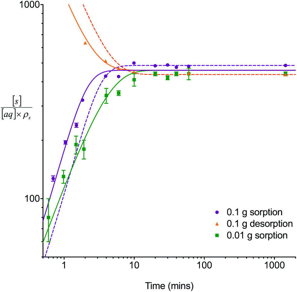 | ||
Fig. 3 Comparison between experimental data (individual data points with error bars) and numerical simulation of sorption/desorption of uranium between 8 M HNO3 and UTEVA resin. The numerical simulation method used input parameters based on an aqueous volume of 10 mL for each experiment. The solid lines represent simulations using rate constants based on the 0.01 g dataset  and an average kD value over the three datasets and an average kD value over the three datasets  . The dashed lines represent input parameters based on the initial and final data points obtained under a particular experimental condition (0.1 g sorption or 0.1 g desorption). . The dashed lines represent input parameters based on the initial and final data points obtained under a particular experimental condition (0.1 g sorption or 0.1 g desorption). | ||
The experimental results showed that the time taken to reach equilibrium was dependent on the solid/aqueous ratio with equilibrium being reached for both analytes in ∼10 minutes using a ratio of 0.1 g solid/10 mL aqueous. The average distribution constant (kD) values were 460 ± 50 and 600 ± 100 for uranium and thorium respectively. These values are similar to previously published data11 for UTEVA resin (the quoted k′ for U(VI) in 8 M HNO3 being ∼300, and the quoted k′ for Th(IV) in 8 M HNO3 being ∼200; kD/k′ = 1.665).
Initially, the numerical simulation rate constants were calculated for each dataset individually. For sorption experiments,  was calculated from the initial slope of concentration change in the solid phase divided by the initial concentration in the aqueous phase. Dividing the concentration ratio (solid/aqueous) after the longest mixing duration by the forward rate constant gave
  . For desorption experiments,
  was calculated from the initial slope; this was then divided into the concentration ratio after the longest mixing duration to obtain
  . For the solid/aqueous ratio of 0.1 g/10 mL, this approach was able to simulate the thermodynamic position of equilibrium but underestimated the initial rate of sorption/desorption due to the practical difficulties of conducting batch experiments with mixing times shorter than 30 seconds. As the initial slope of sorption/desorption decreases with decreasing Vs/Vaq due to a lower proportion of complexant molecules, a better estimation of
  can be achieved using the 0.01 g solid/10 mL aqueous sorption datasets.
The goodness of fit between the experimental and simulated data (Table 2) was assessed using normalised standard deviation analysis (eqn (13)) where n is the number of data points (negative or zero experimental sorption values are excluded). This analysis indicated that the single analyte numerical simulation gave a better description of the interaction of uranium and thorium with UTEVA resin in 8 M HNO3 when  is based on the 0.01 g resin dataset.
 | (13) |
 and the average kD value over the three datasets
| Analyte | Solid mass (g) | Notes | Δq (%) | |
|---|---|---|---|---|
| Rate constants based on each dataset | Rate constants based on 0.01 g dataset and average kD value | |||
| Uranium | 0.1 | Sorption | 23 | 8 |
| 0.1 | Desorption | 23 | 4 | |
| 0.01 | Sorption | 9 | 10 | |
| Thorium | 0.1 | Sorption | 23 | 13 |
| 0.1 | Desorption | 18 | 6 | |
| 0.01 | Sorption | 13 | 17 | |
3.2. Batch experiments – multiple analyte numerical simulation
A series of isotherm experiments using 8 M HNO3 solutions containing only a single interacting species at varying concentrations were conducted to determine the lumped solid extractant concentration model constant (Fig. 4). At low initial aqueous concentrations (<1 × 10⁻⁴ mol L−1) the concentration on the lumped solid phase at equilibrium exhibited a linear relationship with the initial concentration in the aqueous phase as seen in the constant sorption value at equilibrium. At high initial aqueous concentrations (>0.01 mol L−1) the concentration on the lumped solid phase at equilibrium tended towards a constant value indicating saturation of the complexant molecules. The value for uranium was approximately double that of thorium although large uncertainties were present when measuring concentration changes after sorption equilibrium had been obtained at high initial aqueous concentrations. An input parameter for [s]E was calculated as 1.5 mol L−1 and the simulation was run for each analyte at a range of aqueous concentration inputs whilst constraining the other species inputs to zero. Comparing the generated sorption values at equilibrium with the experimental data gave a good fit for both uranium (Δq (%) = 15%) and thorium (Δq (%) = 27%).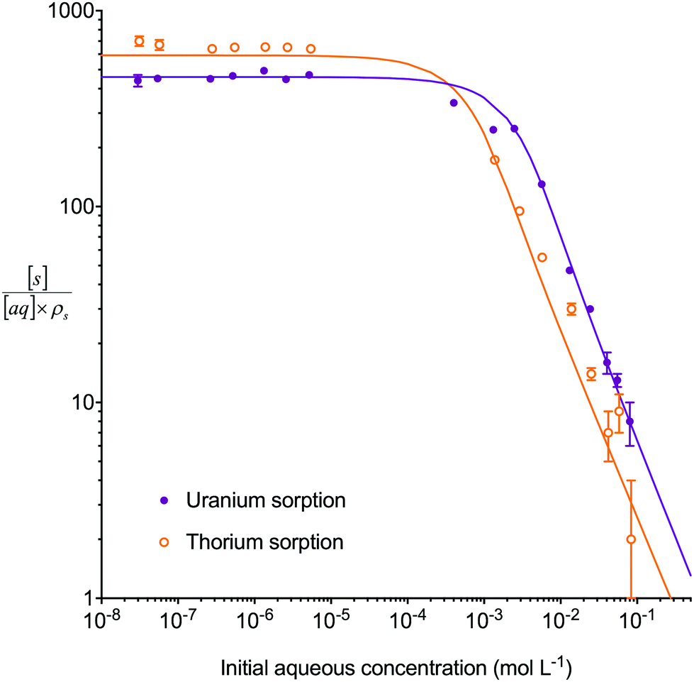 | ||
| Fig. 4 Comparison between experimental data (individual data points with error bars) and numerical simulation of uranium and thorium sorption equilibrium positions between 8 M HNO3 and UTEVA resin at a range of initial aqueous concentrations. The solid lines represent the final values obtained from simulations using differential equations including both species as well as a lumped solid extractant concentration model constant of 1.5 mol L−1 (eqn (8)–(11)). The numerical simulation method used input parameters based on an aqueous volume of 10 mL and a solid mass of 0.1 g for each experiment. The initial aqueous concentration of the species not being simulated was constrained to zero. | ||
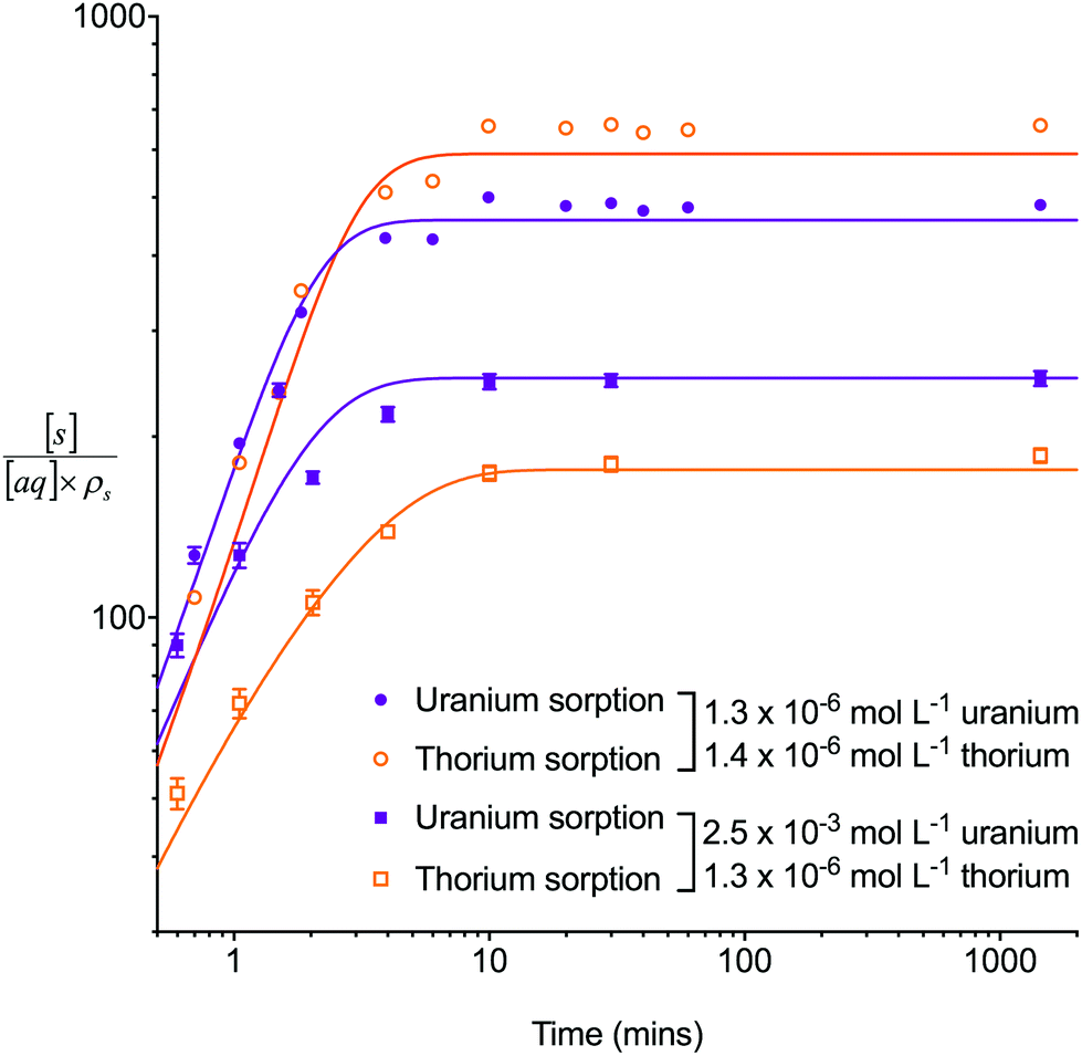
The multiple analyte numerical simulation method with [s]E = 1.5 mol L−1 was also applied to batch sorption experiments with either a high concentration of uranium (2.5 × 10⁻³ mol L−1) and a low concentration of thorium (1.3 × 10⁻⁶ mol L−1) or a low concentration (∼1 × 10⁻⁶ mol L−1) of both analytes (Fig. 5). A solid/aqueous ratio of 0.1 g/10 mL and 8 M HNO3 as the aqueous matrix were used in both experiments. The high concentration of uranium caused a decrease in the kD values of both uranium and thorium in comparison to the low concentration solution. This dataset, therefore, provides kinetic information on the effect of high analyte concentration as well as the effect of a competing interferent. The multiple analyte numerical simulation approach accurately predicted the change in kinetics for both analytes with Δq (%) values for the high uranium solution of 11% (uranium) and 6% (thorium) whereas the single analyte method generated datasets unchanged from the low uranium solution values.
 | ||
| Fig. 5 Comparison between experimental data (individual data points with error bars) and numerical simulation of sorption of uranium and thorium between 8 M HNO3 and UTEVA resin using different initial uranium concentrations. The solid lines represent simulations using differential equations including both species as well as a lumped solid extractant concentration model constant of 1.5 mol L−1 (eqn (8)–(11)). The numerical simulation method used input parameters based on an aqueous volume of 10 mL and a solid mass of 0.1 g for each experiment. No external mass transfer was included. | ||
3.3. Column experiments – small volume loading at slow flow rates
Simulations were run to describe a series of discrete loading breakthrough experiments for UTEVA resin using a bed length of 2 cm and flow rates of <2 mL min−1 (controlled using a peristaltic pump). These experiments involved the loading of a small volume (25 μL) followed by a wash step using the same matrix as the loading solution (8 M HNO3). As the loading and wash solutions were identical, no changes to the rate constants were made between the two steps. The loading concentration used was ∼1 × 10⁻⁴ mol L−1 for both analytes which is within the linear part of the sorption isotherm (Fig. 4).Under these conditions, the strong retention and fast kinetics generated approximately Gaussian shaped experimental profiles for both analytes with a slightly longer tailing slope than the leading slope.
| Expt. | Flow rate (mL min−1) | Axial division length (cm) | Uranium | Thorium | Overall fit | ||
|---|---|---|---|---|---|---|---|
| Slope | R 2 | Slope | R 2 | ||||
| 1 | 0.125 | 0.2 | 0.6413 | 0.6497 | 0.6937 | 0.5222 | 0.15 |
| 0.1 | 0.7812 | 0.7340 | 0.8772 | 0.9192 | 0.46 | ||
| 0.08 | 0.8192 | 0.7184 | 0.9344 | 0.9633 | 0.53 | ||
| 0.05 | 0.8827 | 0.6413 | 1.0445 | 0.9694 | 0.53 | ||
| 0.01 | 0.9545 | 0.3849 | 1.2132 | 0.7855 | 0.24 | ||
| 2 | 0.230 | 0.2 | 0.6519 | 0.7428 | 0.7598 | 0.7673 | 0.28 |
| 0.1 | 0.8234 | 0.9154 | 0.9692 | 0.9527 | 0.70 | ||
| 0.08 | 0.8758 | 0.9261 | 1.0342 | 0.9663 | 0.76 | ||
| 0.05 | 0.9728 | 0.8977 | 1.1489 | 0.9549 | 0.73 | ||
| 0.01 | 1.0987 | 0.7685 | 1.2770 | 0.8895 | 0.49 | ||
| 3 | 0.321 | 0.2 | 0.6885 | 0.6251 | 0.7758 | 0.8027 | 0.27 |
| 0.1 | 0.7611 | 0.4744 | 0.8512 | 0.7528 | 0.23 | ||
| 0.08 | 0.7719 | 0.4117 | 0.8601 | 0.7029 | 0.19 | ||
| 0.05 | 0.7806 | 0.3044 | 0.8634 | 0.6104 | 0.13 | ||
| 0.01 | 0.7790 | 0.2023 | 0.8552 | 0.5176 | 0.07 | ||
| 4 | 1.89 | 0.2 | 0.9387 | 0.9775 | 1.0691 | 0.9456 | 0.81 |
| 0.1 | 0.9791 | 0.9985 | 1.1004 | 0.9778 | 0.87 | ||
| 0.08 | 0.9847 | 0.9991 | 1.1044 | 0.9803 | 0.87 | ||
| 0.05 | 0.9904 | 0.9997 | 1.1089 | 0.9837 | 0.88 | ||
| 0.01 | 0.9944 | 0.9997 | 1.1117 | 0.9853 | 0.88 | ||
The simulated profiles were compared to the experimental results by plotting the simulated value (y axis) against the experimental value (x axis) for the closest possible breakthrough fraction (mL). A linear trendline was applied to the resulting plot and forced through the origin. Regression analysis of the trendline generated a slope value and an R2 value. The slope value gives information on the agreement between the peaks of the two datasets; an exact match between the two datasets would give a slope value of 1. The R2 value gives information on agreement between the shapes (width and symmetry) of the simulated and experimental datasets. It should be noted, however, that the experimental concentration values are given for the mid-point of a collected volume so are averaged over a larger volume than the simulated data (averaged over 0.1 mL). An overall fit score was also calculated by multiplying the slope and R2 values for both analytes (1 per slope was used if slope was >1). An overall fit greater than 0.8 was categorised as corresponding to a very good agreement between the simulated and experimental datasets whereas an overall fit less than 0.2 was categorised as corresponding to a very poor agreement.
The experiment run at 0.321 mL min−1 (experiment 3) showed a poor fit to the simulated datasets using any axial division length input and was subsequently excluded from optimisation analysis. The experimental data showed earlier breakthrough peaks for both analytes than predicted by the numerical simulation method which could be due to inaccurate input parameters (see section 3.3.2.).
At a flow rate of 1.89 mL min−1 (experiment 4), selecting an axial division length of 0.1 cm or less gave a comparable fit to the experimental data. At the slower flow rates of 0.230 mL min−1 (experiment 2) and 0.125 mL min−1 (experiment 1), however, inputting an axial division length of <0.05 cm caused inaccurate narrowing of simulated peaks. The optimal axial division length was therefore determined to be 0.08 cm. This estimation could be improved with further experiments. It has also been suggested that eddy dispersion may not be independent of flow rate.10 For example, a variation on the Van Deemter equation (eqn (1)) known as the Knox equation9 proposes Aue1/3 as the eddy dispersion term. The homogeneity of the packed bed and any changes to structure over the course of the separation procedure may also impact fluid pathways. It should also be noted that, as it dictates the array dimensions, the number of axial divisions must be an integer; if the bed length is not divisible by the axial division length then the number of divisions is rounded up and the length of the axial divisions is slightly less than the determined value.
Diffusion coefficients (DA) of 0.620 × 10⁻⁵ cm2 s−1 for ⅓Ce3+ (proxy for Th4+) and 0.426 × 10⁻⁵ cm2 s−1 for ½UO22+ in water at 25 °C are published.12 As the rate of molecular diffusion is dependent on molecular radius and viscosity, these values are estimates. Using these estimates and the optimised axial division length, aqueous diffusion rate constants (kdiff) can be calculated (eqn (14)).
 | (14) |
These values are then programmatically input into a modified differential equation for the change in analyte concentration in the aqueous phase of axial division z (eqn (15)). The proportion following either sorption/desorption or molecular diffusion would depend on the difference in concentration between the phases/divisions and the competing rate constants. As with the numerical simulation method for column breakthrough not including axial diffusion (section 2.5.3.), each iteration of the ODE solver represents a set simulation time which is dependent on flow rate (eqn (12)).
 | (15) |
Numerical simulations using this modified coding indicate that molecular diffusion causes a significant broadening of breakthrough profiles and change in the position of peak breakthrough at flow rates less than 0.02 mL min−1. Although diffusion rates are affected by solution matrix and the geometry of the packed bed, the estimated value at which molecular diffusion becomes important is much lower than flow rates likely to be used in laboratory-based radioanalytical separations. The exclusion of molecular diffusion from the numerical simulation method reduces the chromatographic breakthrough computation time.
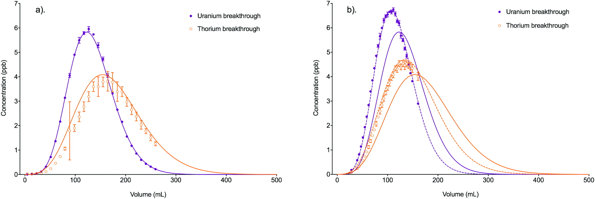 | ||
Fig. 6 Comparison between experimental data (individual data points with error bars) and numerical simulation of uranium and thorium breakthrough profiles from UTEVA resin in 8 M HNO3 for two identical experiments. The two analytes have been simulated simultaneously under conditions corresponding to experiment 4/5 (Table 4). The numerically simulated data using parameters derived from the batch experiments (solid lines) has been compared to (a) experiment 4 and (b) experiment 5. For experiment 5, the simulation with the best overall fit (increased  ) is also shown for comparison (dashed lines). ) is also shown for comparison (dashed lines). | ||
| Expt. | Uranium | Thorium | Overall fit | ||
|---|---|---|---|---|---|
| Slope | R 2 | Slope | R 2 | ||
| 4 | 0.9847 | 0.9991 | 1.1044 | 0.9803 | 0.87 |
| 5 | 0.8399 | 0.7621 | 0.8158 | 0.9610 | 0.50 |
The worse fit for experiment 5 could be due to small differences in the experimental conditions leading to inaccurate input parameters. This possibility has been explored by altering the numerical simulation input parameters relating to the packed bed dimensions, flow rate, solution density and position of equilibrium to obtain a good fit to the experiment 5 dataset (Table 5). This provides insight into the sensitivity of the numerical simulation method to changes in input parameters and the level of accuracy needed when measuring or estimating these values.
| Bed length (cm) | V aq | Column radius (cm) | Flow rate (mL min−1) | Density (g mL−1) | [s]E | Rate constants | Overall fit |
|---|---|---|---|---|---|---|---|
| 2 | 0.655 | 0.35 | 1.89 | 1.25 | 1.5 | Unchanged | 0.50 |
| 1.75 | 0.655 | 0.35 | 1.89 | 1.25 | 1.5 | Unchanged | 0.90 |
| 2 | 0.7 | 0.35 | 1.89 | 1.25 | 1.5 | Unchanged | 0.89 |
| 2 | 0.655 | 0.327 | 1.89 | 1.25 | 1.5 | Unchanged | 0.90 |
| 2 | 0.655 | 0.35 | 4.8 | 1.25 | 1.5 | Unchanged | <0.2 |
| 2 | 0.655 | 0.35 | 2.15 | 1.1 | 1.5 | Unchanged | 0.91 |
| 2 | 0.655 | 0.35 | 1.89 | 1.25 | 1.45 | Unchanged | 0.79 |
| 2 | 0.655 | 0.35 | 1.89 | 1.25 | 1.5 |
 is 1.15 times smaller
|
0.89 |
| 2 | 0.655 | 0.35 | 1.89 | 1.25 | 1.5 |
 is 1.15 times greater
|
0.94 |
The percentage reduction in bed length required to achieve a good fit to the experimental data is greater than the percentage reduction in column radius required. This is due to the relative contribution of each of these factors to the duration of solution residence time in the column (eqn (12)). As the column radius is squared, a smaller percentage error makes a larger difference to the volume of the total aqueous phase than a similar error in the bed length.
The bed length was measured to the nearest 0.05 cm so it is unlikely that an error of 0.25 cm (to give a bed length of 1.75; see Table 5) could have been made in the measurement. The internal diameter of the column is less easily measured; dissection of a column and the use of callipers gave a diameter of 0.683 cm at the bottom of the column, 0.713 cm around the middle and 0.760 cm at the top of the available packed bed region (before the column broadens to accommodate a reservoir of solution). These measurements indicate that the columns used in these experiments taper and the single column radius input may be an oversimplification. Shorter bed lengths would also have a smaller average column radius than longer beds. The column radius of 0.327 cm (Table 5) needed to fit the experimental data is, however, even smaller than that measured at the lower region of the column. As the internal dimensions of only one column were measured, there could be some additional unaccounted variation between experiments.
A reduction in aqueous volume fraction would also reduce the solution residence time in the column giving less time for transfer onto/from the solid phase. The associated increase in solid volume fraction would, however, increase the interphase area allowing for a greater flux between the two phases. The effect of errors in the solid/aqueous ratio is therefore more complex. Under these conditions, a drop from 0.345/0.655 to 0.3/0.7 is needed to achieve a good fit to the experimental data. The original ratio (measured by volumetric displacement) is closer to the published free column volume (Vaq) of 0.65 mL mL−1.11
Depending on the flow rate, fluid pressures may compress the packed bed. This would decrease the bed length and increase the solid/aqueous ratio. As these two changes appeared to have opposing effects it is hard to estimate the net effect on the breakthrough profile. Another possible physical change is the swelling or shrinking of the particles. If the electrostatic forces keeping the UTEVA resin particles in their loosely packed structure were unaffected, this could change both the available interphase area and bed length without altering the solid/aqueous ratio. Swelling or shrinking is normally seen after changes to the aqueous environment such as pH or acid concentration changes. To minimise physical changes due to bed compression, shrinking or swelling, the packed bed was always preconditioned by pumping the same matrix as the loading solution through the column at a moderate flow rate (∼2 mL min−1) for 5 minutes. The bed length measurement was made after this procedure.
Another phenomenon that is unaccounted for in bed dimensions and phase fraction inputs is the presence of air bubbles. Although the practice of slurry packing and capping of the column during set-up to avoid the bed drying out both help avoid the formation of bubbles, some may still be present. This would impact on the available aqueous phase volume without affecting the other measured dimensions. Non-uniform packing could also lead to preferential paths within the resin bed. This channelling may become more prevalent at higher flow rates.
In order to accurately simulate the position of the experimental breakthrough peak, the flow rate had to be increased from 1.89 mL min−1 to 4.8 mL min−1. This change also significantly broadened the shape of the breakthrough profile for both species leading to negative R2 values which inhibited the calculation of a meaningful overall fit value. As the calculated standard deviation on the average flow rate was 0.01 mL min−1, such a large difference in input parameters is a very unlikely cause of the difference in breakthrough profiles between experiments 4 and 5. Another factor in the calculation of the average volumetric flow rate was the density of the solution. The density of 8 M HNO3 at room temperature (1.25 g mL−1)12 was used in the calculation of the flow rate input value and the volume of each collected fraction. A better fit between the experimental and simulated datasets was achieved by using a density of 1.1 g mL−1; this altered the volumetric position of the breakthrough peak in both sets of data. This would correspond to a molarity of ∼3 M which is far outside the expected uncertainty range on the laboratory prepared solution.
A lower ([s]E) value would imply a loss of the immobilised organic extractant from the resin prior to the start of the breakthrough experiment or a difference in extractant concentration between batches of resin. Whilst leaching of organic extractant during storage in slurry form is possible, the best overall fit obtained via variation of the [s]E input parameter was only 0.79. A good fit could not be achieved for both analytes simultaneously by varying [s]E due to the different stoichiometric relationships of the two analytes with the extractant.
The rate constants for UTEVA resin used thus far have been based on kD values of 459 for uranium and 592 for thorium (in 8 M HNO3). The range of both of these values measured over all batch experiments conducted was quite large however, with an uncertainty on the average values of 51 for uranium and 127 for thorium (2sd). In order for the numerical simulation method to generate a breakthrough profile with the analyte peaks occurring earlier, the kD values must be smaller. This was achieved by either reducing the forward rate constants or increasing the reverse rate constants to achieve kD values of 399 for uranium and 515 for thorium.
The simulated breakthrough profiles using an increased reverse rate constant gave a better description of the experimental datasets for both uranium and thorium with the best overall fit of any of the fitted parameter simulations (Fig. 6b). Although the simulated breakthrough profiles generated using the decreased forward rate constant gave a comparable prediction of the volume at which maximum breakthrough concentration occurred, the shapes of the breakthrough profiles were broader and less accurate. Batch experiments varying the HNO3 concentration over the range 7 M–9 M showed opposing relationships between kD and HNO3 concentration for the two analytes. The effect of temperature on kD has not been investigated in this study although Janda et al.13 showed UTEVA extraction efficiency to be significantly reduced when performing sorption experiments at temperatures outside the typical laboratory range.
An increase in  could also be due to in situ leaching of extractant providing a secondary mechanism for complexed analyte transfer down the column. Evidence for this phenomenon has been observed for other extraction chromatographic resins either directly through measurement of organic species in the effluent14 or indirectly through loss of efficiency on repeated use of the same resin bed.15 The extent of leaching was also suggested to be related to flow rate16 and could be reduced by saturating the chromatographic reagents with the organic phase solvent.17 An evaluation of extractant loss was also carried out by Horwitz et al. in their initial characterisation of UTEVA resin.11 After washing a column with ∼100 free column volumes of 2 M HNO3, analysis of the effluent for phosphorus indicated a total extractant loss of 5.8%. The relationship between flow rate and the mobilisation of organic solvent from UTEVA resin could be explored by measuring the extractant concentration present in collected fractions. The extent of extractant loss is also important when considering regeneration and reusability of the sorptive material.
3.4. Column experiments – small volume loading at fast flow rates
Faster flow rates and shorter columns produced a higher degree of tailing in the experimental datasets with less wash solution required to reach peak breakthrough concentration. Although this was reflected in the simulated data, an initial spike was also generated which was not seen in the experimental data even if corrections were made for dilution of the small concentrated volume in a larger, more dilute volume. The size of this spike increased with flow rate. In addition, simulations of breakthrough profiles at the fastest flow rates (>5 mL min−1) significantly misrepresented the shape of the leading slope.The initial spike could be due to an improper representation of flow rates at the beginning of the experiment. A delay of up to one minute occurred between pipetting the solution (0.025 mL) on to the top of the upper frit, reattaching the lid and commencing pumping. During this time, the dissolved species may be able to pass through the frit via diffusion or gravity induced flow into the top axial division of the packed bed.
A low estimate of ∼10 seconds delay in the uppermost axial division was therefore included in the numerical simulation by programming a flow rate of 0.15 mL min−1 for the iteration after addition of the discrete loading volume before returning to the average flow rate for that experiment. This modification greatly reduced the size of the initial spike for both uranium and thorium breakthrough profiles, completely removing it in the slower flowing experiments (experiments 6 and 7). In addition to this change, the delay modification caused a shift in the position of the maximum breakthrough concentration to a later volume fraction thereby reducing the overall fit between the simulated and experimental datasets in most cases (Table 6).
| Expt. | Bed length (cm) | Flow rate (mL min−1) | Delay modification? | Uranium | Thorium | Overall fit | ||
|---|---|---|---|---|---|---|---|---|
| Slope | R 2 | Slope | R 2 | |||||
| 6 | 1 | 2.12 | No | 0.7804 | 0.9680 | 0.7761 | 0.9679 | 0.57 |
| Yes | 0.6965 | 0.8932 | 0.6275 | 0.9083 | 0.35 | |||
| 7 | 1.1 | 3.60 | No | 0.8919 | 0.8815 | 0.8962 | 0.3352 | 0.24 |
| Yes | 0.8123 | 0.8662 | 0.7514 | 0.9006 | 0.48 | |||
| 8 | 1 | 5.48 | No | 0.9275 | 0.6477 | 0.8915 | 0.1881 | 0.10 |
| Yes | 0.8664 | 0.1906 | 0.8165 | −0.6551 | <0.2 | |||
| 9 | 3.9 | 28.8 | No | 0.7498 | 0.7746 | 0.7535 | 0.7182 | 0.31 |
| Yes | 0.7123 | 0.6515 | 0.7434 | 0.3190 | 0.11 | |||
It was also observed that the flow rate in the first collected fraction for these four experiments was lower than the average flow rate through the rest of the experiment. This gradual build-up of flow rate could be due to the competing processes of backpressure and compression of the air in the volume above the column. An accumulation of solution in this headspace volume was visible at the highest flow rates.
An estimation of the gradual build-up of flow rate was made for the experiment run at the fastest flow rate (experiment 9). The LabVIEW code was modified to include this estimation by programmatically setting 6 lower flow rates for a set number of iterations prior to the final average flow rate of 28.8 mL min−1. This modification generated simulated breakthrough profiles without an initial spike for both uranium and thorium. The programmed step changes in flow rate are seen in the shape of the leading slope. The position of the simulated breakthrough peak and shape of the tailing slope were later than the experimental data and very similar to those simulated when applying the ∼10 s delay modification although the overall fit was slightly improved (Table 7).
| Rate constants | Uranium | Thorium | Overall fit | ||
|---|---|---|---|---|---|
| Slope | R 2 | Slope | R 2 | ||
| Unchanged | 0.7204 | 0.6821 | 0.7506 | 0.3871 | 0.14 |
 is 1.64 times greater is 1.64 times greater |
0.9994 | 0.9828 | 1.0501 | 0.9733 | 0.91 |
As in situ extractant leaching was proposed as the most likely cause of peaks in experimental breakthrough profiles appearing earlier than simulated, the  input values were increased to fit the experimental data (Fig. 7). These fitted values corresponded to a decrease in kD from 459 to 280 for uranium and from 592 to 361 for thorium. These amended distribution constants are outside the range observed under the batch conditions. This could be due to the fast flow rate increasing the extent of solvent leaching.
 | ||
Fig. 7 Comparison between experimental data (individual data points with error bars) and numerical simulation of uranium and thorium breakthrough profiles from UTEVA resin in 8 M HNO3 using a programmed build-up of flow rate. The two analytes have been simulated simultaneously under conditions corresponding to experiment 9 (Table 6) but are displayed separately for clarity. A gradual build-up of flow rate has been programmatically simulated using either rate constants determined from batch sorption/desorption data (solid line) or where  has been increased by a factor of 1.64 (dashed line). has been increased by a factor of 1.64 (dashed line). | ||
3.5. Column experiments – large volume and/or high concentration loading
For the experimental breakthrough profiles described thus far, the loading volume has been small (0.025 mL) and the uranium and thorium concentrations in the loading solution low (∼1 × 10⁻⁴ mol L−1). The majority of interactions are therefore happening at concentrations within the linear part of the sorption isotherm. This means that the stoichiometric relationship between the analytes and the extractant is not expected to have an impact on the simulated breakthrough profiles. This could be tested by simplifying the LabVIEW coding to only simulate one analyte at a time and to not include the lumped solid extractant concentration model constant (eqn (2) and (3)). If the amount of analyte loaded on to the column is sufficiently high in relation to the column length, the single analyte method is expected to generate less accurate chromatographic predictions than the more complex multiple analyte method.The single analyte and multiple analyte numerical simulation methods were compared to experimental datasets for the breakthrough of uranium and thorium in 8 M HNO3 from UTEVA resin at a range of loading volumes and loading concentrations (Table 8). The bed length and flow rate were kept to values that were known to produce breakthrough profiles that could be simulated without inclusion of aqueous phase diffusion or gradual build-up of flow rate.
| Expt. | Bed length (cm) | Flow rate (mL min−1) | Loading volume (mL) | Uranium loading concentration (mol L−1) | Thorium loading concentration (mol L−1) | Overall fit | |
|---|---|---|---|---|---|---|---|
| Single analyte | Multiple analyte | ||||||
| 4 | 2 | 1.89 | 0.025 | 1.33 × 10⁻⁴ | 1.39 × 10⁻⁴ | 0.87 | 0.87 |
| 10 | 1.95 | 1.59 | 1.004 | 1.32 × 10⁻⁴ | 1.36 × 10⁻⁴ | 0.86 | 0.89 |
| 11 | 2 | 1.82 | 258.59 | 5.06 × 10⁻⁷ | 5.23 × 10⁻⁷ | 0.86 | 0.87 |
| 12 | 1.95 | 1.56 | 0.025 | 2.70 × 10⁻³ | 1.36 × 10⁻⁴ | 0.93 | 0.93 |
| 13 | 2.1 | 1.86 | 24.64 | 2.51 × 10⁻³ | 1.56 × 10⁻⁴ | <0.2 | 0.63 |
For experiments with either a low loading volume or concentration (experiments 4 and 10–12), both numerical simulation methods gave sufficiently accurate descriptions of the breakthrough profiles. For a higher loading concentration of uranium and a moderately large loading volume (experiment 13), the single analyte method completely failed to describe the experimental dataset.
A change in the shape of the breakthrough profiles is observed when comparing small loading volumes of 0.025 mL (experiment 4) and 1.004 mL (experiment 10) to a large loading volume of 258.59 mL (experiment 11) whilst keeping the concentrations of both analytes low (Fig. 8). The increase in loading volume from 0.025 mL to 1.004 mL caused an increase in the height of the breakthrough profiles but not a significant change in the position or shape of the peak. The slight differences between the simulated breakthrough peaks are due to small differences in bed length, flow rate and loading concentrations between the two experiments. At the large loading volume of 258.59 mL, the concentration of both uranium and thorium in the column outlet fractions keeps rising beyond the peak position seen for the smaller loading volumes. The breakthrough profiles for both species are wider and more asymmetrical with the peak for uranium showing a plateau in concentration. These shapes are depicted in the experimental and numerically simulated datasets although the simulated profiles are shifted to slightly later positions.
 | ||
| Fig. 8 Effect of increased loading volume on uranium and thorium breakthrough profiles. The two analytes have been simulated simultaneously. The upper plot shows simulated datasets corresponding to experiments 4 and 10 (Table 8). The simulated breakthrough profiles for experiment 4 (solid line) are plotted on the left hand axis and those for experiment 10 (dashed line) are plotted on the right hand axis. The lower plot shows simulated and experimental datasets corresponding to experiment 11 (Table 8). The vertical dotted line shows the volume at which the column input was switched from the loading solution to the wash solution. | ||
An increase in the concentration of uranium in the loading solution of approximately 20 fold did not significantly change the position or shape of the experimental breakthrough profiles for either uranium or thorium when the loading volume was small (0.025 mL, experiments 4 and 12). Again, the slight differences in the position and width of the simulated breakthrough peaks are due to the small differences in bed length, flow rate and loading concentrations between the two experiments. Using a much larger loading volume of 24.64 mL (experiment 13), however, this elevated uranium concentration did have an impact on the peak position and shape of the breakthrough profiles for the experimental datasets for both analytes (Fig. 9). The peak positions are earlier than would be expected if the stoichiometric relationship between the analytes and the extractant was not considered; i.e., the single analyte numerical simulation method. In addition, the experimental datasets for both species are more asymmetrical than the single analyte simulations with a longer tailing slope and a shorter leading slope. These observations indicate that the concentration of complexant molecules in the extractant is a limiting factor under these experimental conditions and must therefore be included in the numerical simulation method.
 | ||
| Fig. 9 Effect of increased loading concentration on uranium and thorium breakthrough profiles. The upper plot shows simulated datasets corresponding to experiments 4 and 12 (Table 8). The simulated breakthrough profiles for experiment 4 (solid line) and thorium for experiment 12 (dashed line) are plotted on the left hand axis and uranium for experiment 12 (dashed line) is plotted on the right hand axis. The two analytes have been simulated simultaneously. The lower plot shows simulated and experimental datasets corresponding to experiment 13 (Table 8). The vertical dotted line shows the volume at which the column input was switched from the loading solution to the wash solution. Datasets simulated using the single analyte method (solid lines) and the multiple analyte method (dashed lines) are shown on this plot. | ||
The total column capacity for a 2 cm long column has been calculated to be 28.5 mg of uranium if using the reference capacity (37 mg mL−1 bed) from the original UTEVA resin characterisation data by Horwitz et al.11 or 47.3 mg if using the lumped solid extractant concentration model constant ([s]E) of 1.5 mol dm−3. For the experiment with an elevated uranium concentration and a small loading volume (experiment 12), the total amount of uranium loaded (1.61 × 10⁻² mg) is significantly below the amount required to saturate the column. For the experiment with a larger loading volume (experiment 13), the total amount of uranium loaded is 14.7 mg. Whilst this is below either estimation of the total column capacity, it is above the recommended loading of 20% total capacity11 and may cause a shift in the breakthrough profiles.
3.6. Application to sequential elution sequences
A typical radioanalytical chromatographic procedure consists of a sample loading step, a rinse step to remove interferents and one or more selective elution steps to isolate the analyte(s) of interest. The rinse step is usually carried out using the same reagent as sample loading whilst subsequent elution steps involve changes in the on-column environment to promote desorption of the analyte from the sorptive material. The recent development of automated radioanalytical techniques means that precise delivery of a sequence of reagents to a column can be made using software control of pumps and valves. The volume and flow rate of each solution can be regulated and the column output either collected or diverted to waste. As the numerical simulation method stores data on the axial distribution of analyte concentration in both the aqueous and solid phases after each iteration of the ODE solver, a change in the column input solution after any specified volume of sample loading and rinse solution could be simulated.The numerical simulation method has been modified to include step changes in eluent and tested using a procedure for the sequential elution of thorium and uranium from UTEVA resin. The experimental sequence consisted of loading both analytes in 8 M HNO3 followed by an 8 M HNO3 rinse step, the elution of thorium using 6 M HCl and finally the elution of uranium using 2% HNO3. This experimental sequence was simulated by addition of a case structure to the LabVIEW coding. The flow rate and rate constant values for each solution were written into separate cases which were selected using the output of a subVI (modular subsection of the LabVIEW coding) that assessed the while loop iteration and assigned a case input value (Table 9). For example, the rinse volume of ∼20 mL was loaded on to the column from iterations 2 ≤ i ≥ 807 during which time a case outputting a flow rate of 1.83 mL min−1 and the forward and reverse rate constant values determined for 8 M HNO3 were selected.
| Sample loading | Rinse | Thorium elution | Uranium elution | ||
|---|---|---|---|---|---|
| Solution | 8 M HNO3 | 8 M HNO3 | 6 M HCl | 2% HNO3 | |
| Flow rate (mL min−1) | 0.15 | 1.83 | 1.83 | 1.83 | |
| Volume (mL) | 0.025 | 19.82752 | 34.57969 | 34.67384 | |
| Iterations | 0–1 | 2–807 | 808–2214 | 2215−end | |
| Concentration (mol L−1) | Uranium | 1.32 × 10⁻⁴ | 0 | 0 | 0 |
| Thorium | 1.36 × 10⁻⁴ | 0 | 0 | 0 | |
| k D | Uranium | 459 | 459 | 400 | 39 |
| Thorium | 592 | 592 | 3.1 | 10.3 | |
The rate constants for 6 M HCl and 2% HNO3 solutions were calculated from a set of batch sorption tests using a ratio of 1 g solid/10 mL solution. This large solid/aqueous ratio allows for a reasonable estimate of distribution constants from weakly interacting analytes. It does, however, make it harder to measure the initial rate of sorption due to equilibrium being obtained in a shorter amount of time.
The calculated distribution constant (kD) values were similar to published values11 with UTEVA resin having a strong affinity for uranium in 6 M HCl (k′ for U(VI) in 6 M HCl ∼200; kD/k′ = 1.665) and a low affinity for uranium in 2% HNO3 (k′ for U(VI) in 0.3 M HNO3 ∼20; kD/k′ = 1.665). The affinity for thorium was low under both conditions (k′ for Th(IV) in 6 M HCl ∼0.9, k′ for Th(IV) in 0.3 M HNO3 ∼5; kD/k′ = 1.665).
The numerical simulation method using the described input parameters gave a moderately accurate description of the experimental dataset (Fig. 10). The difference in elution peak width between the analytes was reflected in the simulated data due to the difference in distribution constants between thorium in 6 M HCl (kD = 3.1) and uranium in 2% HNO3 (kD = 39).
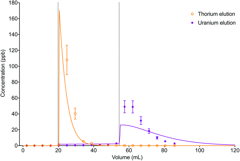 | ||
| Fig. 10 Comparison between experimental data (individual data points with error bars) and numerical simulation of uranium and thorium elution profiles from UTEVA resin using a programmatically input elution sequence (Table 9). Both analytes were simulated simultaneously. The vertical dotted lines show the volumes at which step changes in reagent were made. | ||
The accuracy of the simulated elution profiles could be improved by using a series of experimentally determined chromatographic datasets to obtain a better estimation of the magnitude of the kinetic rate constants. In addition, it may be necessary to use a more realistic model of step changes in reagent in the numerical simulation method. Currently, the rate constant input parameters are changed for every axial division simultaneously. This implies an immediate change in environment (or acid concentration) over the whole column length. Whilst this simplification may produce reasonable results for short columns, the deviation between experimental and simulation datasets is expected to be larger for longer bed lengths. The LabVIEW coding could therefore be modified to better simulate a step change in reagent by replacing the 1D set of rate constants with a 2D array allowing for the new parameters to be introduced at the top axial division and progress down the column. A further complication is that the change in environment (or acid concentration) in each axial division may not be a step change; instead a gradient may form between the existing and new reagents. Intermediate rate constants could be included to simulate this phenomenon.
3.7. Future extension of the numerical simulation method – inclusion of mass transfer
In slow-moving solutions, a concentration gradient can occur around the particle surface due to analyte depletion via sorption combined with a slow rate of mass transfer from the bulk solution. This film diffusion process can be represented in the LabVIEW coding by splitting the aqueous volume into a bulk fraction and a surface fraction. This modification could be used to simulate batch sorption under alternative geometries such as a probe coated with a thin film of sorptive particles (dip stick technologies).18For radiochemical extraction chromatographic resins consisting of a solvent extractant immobilised on a solid support, internal diffusion is not a rate determining step. For porous materials such as ion exchangers, however, intraparticle diffusion can cause a slowing of the rate of sorption after the initial transfer of species between the aqueous phase and the surface of the solid particles. Internal diffusion could be included in the numerical simulation method by splitting the lumped solid fraction up into two or more sections. This would also increase the amount of model constants, input and output variables as well as the number of differential equations used by the ODE solver thereby increasing the computing time.
4. Conclusions
Development of the numerical simulation method in LabVIEW benefitted from the modular and graphical nature of the programming environment. Modification of the basic simulation by extending arrays, adding connections, duplicating, and editing VIs was relatively simple. The ODE solver, however, required the differential equations to be in certain formats to avoid mass balance errors. For example; kint[s]outer − kint[s]inner was acceptable whereas kint([s]outer − [s]inner) generated incorrect concentrations.The numerical simulation method shows potential for development into user-friendly software for use as a radioanalytical tool. Publication of a LabVIEW project as software removes access to the block diagram coding, leaving only the front panel user interface of the main VI. The end-user would be able to control a selection of input variables and view the results of the simulation either via an on-screen graph or as an exported dataset accessible using common spreadsheet applications (e.g. Microsoft Excel). The ability to vary the column dimensions (bed length and column radius), flow rate and sample loading conditions (analyte concentration and volume) and observe the impact on breakthrough profiles would help to streamline the radioanalytical method development process and reduce the amount of experiments required. This is particularly important for supporting the development of rapid and automated radioanalytical techniques where chromatographic column flow is increased above the rate at which the separation procedure was originally characterised.
Regardless of the exact nature of a potential chromatographic simulation tool for radiochemical analysts, a few features are likely to be required (Table 10). As LabVIEW is a visual programming language, it is easy to display these controls and indicators in an intuitive graphical interface.
| Software feature | Possible formats |
|---|---|
| Column radius control | Typed numerical input |
| Bed length control | Typed numerical input (rounded to multiple of axial division length) |
| Resin selection | Drop-down menu |
| Elution sequence control | Input of solution, volume and flow rate in specified order |
| Sample composition | Drop-down menu or numerical input of concentrations |
| Sample and reagent solution selection | Drop-down menu |
| Sample and reagent volume control | Typed numerical input |
| Sample and reagent flow rate control | Typed numerical input (possible upper and lower limit restrictions) |
| Data output | On-screen graph, on-screen value, exported dataset |
Restricting the range of flow rate inputs to values where aqueous phase diffusion and organic solvent leaching are negligible would allow for simpler differential equations and hence quicker simulation time. As one of the main advantages of automated radioanalytical separation systems is the reduced time taken to carry out chromatographic procedures, it is likely that the flow rate through the column would be increased above the rate of gravity flow and therefore sufficiently high enough that aqueous phase diffusion could be ignored. The exception to this situation is if flow through the column is stopped to allow for kinetically slow processes to occur. For example, a pause of at least 7 minutes was required for the complete reduction of Np(IV) to Np(III) in a method for the separation of actinides using TEVA and DGA resins.19 Additionally, very fast flow rates leading to loss of the immobilised solvent extractant would be avoided particularly if the sorptive material was to be reused. This could mean that inclusion of leaching rate in the numerical simulation method would be unnecessary. Further investigations into extractant leaching are needed in order to better simulate chromatographic breakthrough at fast flow rates. The gradual build-up of flow rate when commencing pumping at fast flow rates would be less easy to accurately simulate. It could instead be reduced by employing an alternative column configuration with less dead volume such as pre-packed cartridges.
One potential application of the numerical simulation software is for custom chromatographic separation using an automated radioanalytical system. As control software written in LabVIEW is already in use for automated systems,20–24 it is possible that the elution sequence could be optimised using a numerical simulation method and the resulting sample/reagent volumes and flow rates fed directly in to the linked or integrated control software.
It is proposed that the numerical simulation method could be easily extended to other extraction chromatographic resins covering a wide range of analyte separation procedures. Providing the kinetics of sorption/desorption can be described using a single pair of differential equations, the equation parameters (forward and reverse rate constants, lumped solid extractant concentration, stoichiometric relationship and ratio of solid to aqueous phases) could be programmatically input using a drop-down menu. By using a ring or enumerated control function, selection of an option could programmatically retrieve data from a particular row of an external spreadsheet file relating to that choice. The list of choices would be set by reading from the external file. Using this method, the database of analyte-sorptive material kinetics could be expanded upon without modification of the LabVIEW coding.
For materials exhibiting similar kinetic behaviour to UTEVA resin, the appropriate input parameters can be readily determined by a series of batch experiments following the method outlined in this paper. The accuracy of the method depends on the detail of the description of the experimental and kinetic parameters. It is recommended that as short a mixing time as practically possible with a low solid/aqueous ratio (0.01 g/10 mL) is used to obtain  . The average kD is best calculated from a moderate solid/aqueous ratio (0.1 g/10 mL) if the analyte is strongly retained on the resin under the conditions investigated and a higher solid/aqueous ratio (1 g/10 mL) if the analyte is weakly retained.
A combination of versatility and accessibility will make the proposed numerical simulation software a useful tool for research scientists and radiochemical analysts. The mechanistic nature of the numerical simulation method means that it could also be used to provide a theoretical insight in to commonly used kinetic equations and simpler chromatographic breakthrough models and the conditions under which these equations are valid.
An advantage of the numerical simulation method over simpler models of chromatographic breakthrough is the ability to predict sequences involving multiple species, changes in flow rate or input matrix, volume or concentration depending on the chosen detection method and analytical requirements. Although further work is needed to improve the estimation of rate constants for eluting reagents and better validate the method, the potential to programmatically introduce step changes in reagent has been demonstrated.
Author contributions
Frances M Burrell: conceptualization, formal analysis, investigation, methodology, software, validation, visualization, writing – original draft, writing – review & editing, Phillip E Warwick: conceptualization, funding acquisition, resources, supervision, writing – review & editing, Ian W Croudace: conceptualization, funding acquisition, resources, supervision, writing – review & editing, W Stephen Walters: resources, supervision, writing – review & editing.Conflicts of interest
There are no conflicts to declare.Acknowledgements
This work was partly funded by the United Kingdom's Nuclear Decommissioning Authority (NDA) through a PhD bursary for Frances Burrell, which was administered and supervised through the National Nuclear Laboratory (NNL). GAU-Radioanalytical and the Geochemistry group of the School of Ocean and Earth Sciences, University of Southampton are acknowledged for the contribution of ICP-MS and radiometric facilities.Notes and references
- G. Guiochon, J. Chromatogr. A, 2002, 965, 129–161 CrossRef CAS PubMed.
- R.-M. Nicoud, Chromatographic Processes: Modeling, Simulation, and Design, Cambridge University Press, Cambridge, 1st edn, 2015 Search PubMed.
- G. Alberti, V. Amendola, M. Pesavento and R. Biesuz, Coord. Chem. Rev., 2012, 256, 28–45 CrossRef CAS.
- Z. Xu, J.-G. Cai and B.-C. Pan, J. Zhejiang Univ., Sci., A, 2013, 14, 155–176 CrossRef CAS.
- W. Plazinski, W. Rudzinski and A. Plazinska, Adv. Colloid Interface Sci., 2009, 152, 2–13 CrossRef CAS PubMed.
- W. Rudzinski and W. Plazinski, Appl. Surf. Sci., 2007, 253, 5827–5840 CrossRef CAS.
- A. Roman, PhD thesis, University of Nevada, Las Vegas, 2014.
- D. S. Moon, W. C. Burnett, S. Nour, E. P. Horwitz and A. Bond, Appl. Radiat. Isot., 2003, 59, 255–262 CrossRef CAS PubMed.
- G. Guiochon, in High-Performance Liquid Chromatography Advances and Perspectives Volume 2, ed. C. Horvath, Academic Press, Inc., New York, 1980, pp. 1–56 Search PubMed.
- M. D. LeVan and G. Carta, in Perry's Chemical Engineer's Handbook, ed. D. W. Green and R. H. Perry, McGraw-Hill Education, New York, 8th edn, 2008, pp. 16-1–16-69 Search PubMed.
- E. P. Horwitz, M. L. Dietz, R. Chiarizia and H. Diamond, Anal. Chim. Acta, 1992, 266, 25–37 CrossRef CAS.
- D. R. Lide, CRC Handbook of Chemistry and Physics, CRC Press, Boca Raton, 84th edn, 2003, vol. 5, p. 93 Search PubMed.
- J. Janda, D. Sas and A. Tokárová, J. Radioanal. Nucl. Chem., 2015, 304, 301–312 CrossRef CAS.
- E. P. Horwitz, D. R. McAlister, A. H. Bond and R. E. Barrans, Solvent Extr. Ion Exch., 2005, 23, 319–344 CrossRef CAS.
- K. Kołacińska, E. Chajduk, J. Dudek, Z. Samczyński, E. Łokas, A. Bojanowska-Czajka and M. Trojanowicz, Talanta, 2017, 169, 216–226 CrossRef PubMed.
- Y. Fajardo, E. Gómez, F. Garcias, V. Cerdà and M. Casas, Anal. Chim. Acta, 2005, 539, 189–194 CrossRef CAS.
- J. W. Grate, S. Fadeff and O. B. Egorov, Analyst, 1999, 124, 203–210 RSC.
- P. E. Warwick and I. W. Croudace, J. Radioanal. Nucl. Chem., 2017, 314, 761–766 CrossRef CAS PubMed.
- N. Guérin, K. Nadeau, S. Potvin, J.-M. Hardy and D. Larivière, J. Radioanal. Nucl. Chem., 2012, 295, 1803–1811 CrossRef.
- Y. Miyamoto, K. Yasuda and M. Magara, Analyst, 2015, 140, 4482–4488 RSC.
- D. Barbesi, V. Vicente Vilas, S. Millet, M. Sandow, J.-Y. Colle and L. Aldave de las Heras, J. Radioanal. Nucl. Chem., 2017, 313, 217–227 CrossRef CAS PubMed.
- K. H. Chung, S. Do Choi, G. S. Choi and M. J. Kang, Appl. Radiat. Isot., 2013, 81, 57–61 CrossRef CAS PubMed.
- K. H. Chung, H. Kim, J. M. Lim, Y.-Y. Ji, G.-S. Choi and M. J. Kang, J. Radioanal. Nucl. Chem., 2015, 304, 293–300 CrossRef CAS.
- S. Yoon, W.-H. Ha, S. Park, S.-S. Lee and Y.-W. Jin, J. Radioanal. Nucl. Chem., 2016, 311, 1053–1057 CrossRef.
| This journal is © The Royal Society of Chemistry 2021 |