In silico high throughput screening of bimetallic and single atom alloys using machine learning and ab initio microkinetic modelling

Abstract

The advent of machine learning (ML) techniques in solving problems related to materials science and chemical engineering is driving expectations to give faster predictions of material properties. For heterogeneous catalysis applications, relying on the age-old Sabatier principle, an ab initio in silico high throughput screening of catalyst materials is envisaged, wherein ML based methods show potential to significantly reduce the experimental as well as computation cost. The availability of ML algorithms (in open source libraries like Scikit-Learn) and materials database (like CatApp and Materials Project) further augments this realization. By using these resources, ML models are developed to predict the binding energies of oxygen and carbon on bimetallic alloys and Cu-based single atom alloys (SAAs) using the features of metals that are readily available in the periodic table. Several ML models for predicting oxygen binding energy for AA terminated A₃B alloys are analysed and gradient boosting regression (GBR) is observed to give superior performance with a root mean square error of 0.31 eV in the test. In addition, GBR based ML models are demonstrated to predict the oxygen and carbon binding energies of AB terminated A₃B alloys with a test error of 0.38 eV and 0.35 eV respectively. The binding energy of oxygen and carbon on Cu-based SAAs is predicted with a test error of 0.36 eV and 0.37 eV respectively. Moreover, the computational time for predicting the binding energy using ML is 0.0006 s on a dual-core laptop which is significantly less than the time required for DFT calculations. DFT and ML calculated carbon and oxygen binding energies for the bimetallic A₃B alloys are further used in an ab initio microkinetic model to calculate the turn over frequency (TOF) for ethanol decomposition and non-oxidative dehydrogenation reactions. The TOFs over bimetallic alloys obtained using the ML calculated binding energies follow the same trend as that obtained using the DFT energies, with the TOF values being the same or within an order of magnitude range. This shows that catalyst screening using binding energy as a descriptor can be performed using ML models, bypassing time and resources consuming DFT calculations. This is likely to speed up the process of novel catalyst discovery.

---

1. Introduction

The binding energy of adsorbates on a heterogeneous catalyst surface is the key parameter in determining its catalyst activity. From the time of Paul Sabatier, catalysis has been thought of as an interplay of surface–adsorbate interactions, in which the adsorbate is expected to bind ‘optimum’ with the catalyst surface, neither ‘weak’ nor ‘strong’, to achieve maximum turn-over of the catalytic cycle, resulting in higher reaction rates. While catalytic reactions on the surface are expected to generate several adsorbates, binding of the key adsorbates is thought to be rate controlling.^1–3 In essence, reaction rates are a function of descriptors linked to the binding of adsorbates. In recent times, the success of ab initio density functional theory (DFT) calculations in binding energy estimations has propagated microkinetic models^4–8 in which the binding energy of carbon, oxygen or nitrogen atoms on the catalyst surface is used as a descriptor to determine the turnover frequencies (TOFs).^1,3,4,9–15 For example, in syngas conversion to ethanol, the reaction rates on a series of transition metal catalysts have been represented as a function of the binding energy of the ‘descriptor’ atom (carbon, oxygen and/or nitrogen), in the form of a Sabatier plot.¹⁵ This inherently is possible, since the binding energy of all the reaction intermediates on the surface are linked to the carbon and oxygen binding energies on the surface following linear scaling relationships.^{4,5,9,10,16–19} From the Sabatier plots, one can rationally think of designing a catalyst surface wherein a metal showing weaker binding of the ‘descriptor’ atom may be alloyed with a metal having stronger binding to synthesize bimetallic alloys which may show desired binding of the ‘descriptor’ corresponding to the Sabatier maxima of reactivity.

The proposed thought on catalyst design, essentially, is the recipe for in silico high throughput screening of catalyst materials to come up with bimetallic alloys which are expected to produce desired reactivity in experiments, reducing the number of experiments required in a typical hit and trial approach to synthesize active catalysts.^{4,6,11,19–25} However, in this recipe, the time required for DFT simulations, in general, is a limiting factor, since the quantum mechanical approach to scan the binding sites of an adsorbate on the catalyst surface and corresponding binding energy calculations is computationally expensive.^26–29

To reduce the number of computationally expensive DFT calculations a linear scaling relationship for binding energy between adsorbed species^10,30–33 as well as a Brønsted Evans Polanyi (BEP) scaling relationship^10,17,34,35 between activation energy and reaction energy are widely used in computational heterogeneous catalysts. To speed up the DFT binding energy calculation, the use of neural network based potentials in the open source Atomistic Machine-learning Package (AMP) developed by Peterson et al.³⁶ and the perturbation theory based alchemy approach by Keith et al.³⁷ have shown to be thousands of times faster than conventional DFT and can be important tools for high-throughput screening of heterogeneous catalysts. Herein, an alternative machine learning (ML) approach is presented which can provide the same information on a significantly reduced time scale.

Recent progress in integrating machine learning with data obtained from DFT calculations has opened up a possibility of exploring a whole new way of high throughput catalyst screening. Towards this, efforts to integrate ML and heterogeneous catalysis commonly apply Artificial Neural Networks (ANNs).³⁸ Ulissi et al.^39–42 and Xin et al.^26,27,43 used ANN based models for the prediction of the activity of transition metal based heterogeneous catalysts, whereas Kulik and co-workers^44–47 applied the ANN method for transition metal based organometallics for catalysis as well as to screen spin crossover complexes for potential application as data storage devices, light sensing switches, etc. However, the challenge with training conventional ANNs is the high computation time, which increases further with more number of hidden layers and neurons.⁴⁸ Another disadvantage of ANNs is their low interpretability. With algorithmic developments, improvised ML algorithms can be developed that are sometimes more accurate and much faster than ANNs. One such algorithm is Gradient Boosting Decision Trees (GBDTs)⁴⁹ which incorporates important advantages of decision trees while using “Boosting” to overcome their biggest drawback – poor predictive performance. Decision trees are adaptable and easy to interpret, can handle different types of variables, need very less pre-processing of data and can fit nonlinear relationships accurately.⁵⁰ Boosting is a technique that is used to convert many weak learners to form a single strong learner.⁵¹ The advantages provided by GBDTs have made it one of the most widely used ML algorithms.⁴⁹

In the selection of an ML model, features are an important constituent.²⁷ Once the dataset of various catalysts is available, it has to be described by features that uniquely represent the catalyst and relate it to the target variable. There have been important contributions in this regard to predict the binding energies as a target variable in order to screen bimetallic catalysts. ANNs have been used to predict binding energies using the electronic properties of alloys like d-band centers as features for the model.^26,27 Tree based ensemble algorithms have shown significantly accurate prediction of binding energies of CH₄ related species on Cu-based alloys using only readily available physical properties of metals as features.⁵²

Here, in this study, an ML based model is developed to predict the binding energy of ‘descriptor’ oxygen and carbon atoms on bimetallic alloys of the form A₃B (211 surface). Various ML algorithms are evaluated to put forward the advantage of GBR over others for the supervised regression problem. Additionally, the GBR model is developed to predict the binding energies of oxygen and carbon over copper based single atom alloys (SAAs). The ML model developed using readily available properties of metals as features is observed to predict the binding energy with accuracy equivalent to that of DFT calculations. Also, the computation time required for this ML model prediction is negligible as compared to DFT calculations. The ML predicted binding energies were further used with an ab initio microkinetic model (MKM) to calculate the catalytic rates for two important catalytic reactions: ethanol decomposition¹³ and non-oxidative dehydrogenation (NODH) reactions¹⁵ over the A₃B bimetallic alloys. Both reactions were earlier studied by us in detail by constructing MKMs for understanding the trend in the catalytic activity of transition metals for C–O bond scission in ethanol¹³ and NODH of ethanol to produce acetaldehyde¹⁵ on undercoordinated step (211) sites. Here in this study, the ML calculated binding energies showed similar predictions for the reactivity of bimetallic alloys to those earlier shown by ab initio MKMs. These findings can ultimately be extended to other metal alloys and catalytic reactions to provide a faster way of catalyst screening.

2. Methods

The ML model is trained and tested on a dataset comprised of binding energies of oxygen and carbon over bimetallic alloys. For the A₃B alloys, the binding energies for AA and AB terminated alloys are obtained from CatApp.²⁰ A model representation of the (211) surface of an AA terminated A₃B alloy is shown in Fig. 1(a) and (b). Corresponding images for an AB terminated A₃B alloy are shown in Fig. 1(c) and (d). For Cu-based SAAs, the binding energies are calculated using a plane wave DFT code as implemented in the Vienna ab initio simulation package (VASP-5.3.5 version, University of Vienna).⁵³ The core electrons are described using Vanderbilt ultrasoft pseudopotentials.⁵⁴ Kohn Sham one electron valence states are expanded with a plane wave basis function and truncated at a cut-off energy of 396 eV. A revised Perdew–Burke–Ernzerhof (RPBE) exchange correlation functional developed by Hammer et al.⁵⁵ is used to describe the exchange and correlation contributions for single electron equations. Terrace (111) sites of Cu-based SAAs are modeled using a slab of 4 layers of size 4 × 4. One Cu atom is replaced with a transition metal: Sc, Ti, V, Fe, Co, Ni, Cu, Zn, Y, Zr, Nb, Mo, Ru, Rh, Pd, Ag, Hf, W, Re, Ir, Pt and Au or a p-block element: B, Al, Ga, Ge, In, and Sn. The model geometry representing a Cu-based SAA (111) terminated surface is shown in Fig. 1(e) and (f). Bottom two layers of the model are fixed while the upper half along the adsorbate (C and O) is allowed to relax to represent the surface, sub-surface and bulk mimicking the phenomenon of surface and subsurface restructuring. The final geometry of the optimized binding configurations for C and O over the Cu-based SAA is shown in the ESI, Fig. SI-1 and SI-2.† A Monkhorst–Pack k point grid with a 3 × 3 × 1 mesh is used to sample the irreducible Brillouin zone.⁵⁶ Slabs are periodically repeated with 20 Å vacuum between the slabs to distinctly represent the gas phase adsorption to the surface. Convergence criteria for force and energy are set to 0.05 eV Å⁻¹ and 10⁻⁴ eV, respectively.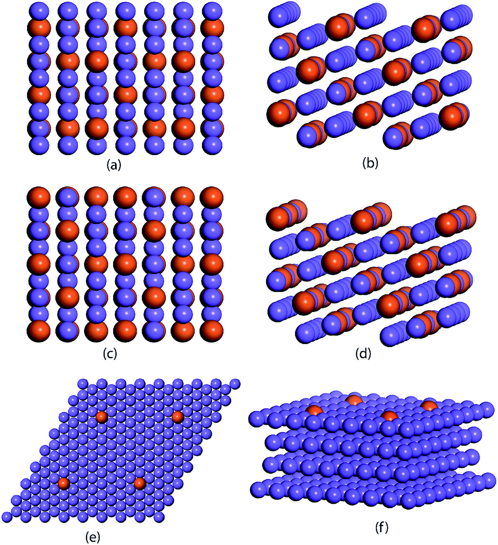

Fig. 1 (a) Top view and (b) side view of the (211) surface of an A₃B bimetallic alloy with AA termination; (c) top view and (d) side view of the (211) surface of an A₃B bimetallic alloy with AB termination; (e) top view and (f) side view of the (111) surface of a Single Atom Alloy (SAA) AB, where B atoms are embedded in the matrix of A metal. Blue color atoms represent the A transition metal and the orange color atom represents the B transition metal/non-metal from the p-block.

Each bimetallic alloy is represented by a set of features that uniquely describe it. For A₃B bimetallic alloys, a set of 27 features are chosen to include the physical properties of both the metals in the alloy. These properties are readily available from the periodic table and other databases.^57–59 Overall, each alloy is depicted by a feature vector comprised of 27 values. For Cu-based SAAs, each alloy is represented by a set of 12 features that include the physical properties of the single atom in the alloy. Features related to Cu are not included as they would be constant for all the SAAs used in the study.

Except ANNs, all other ML algorithms are implemented using the widely used open-source library Scikit-Learn.⁶⁰ ANNs are implemented using Keras⁶¹ with a TensorFlow⁶² backend. For evaluating the predictive power of the ML algorithms, the dataset is first split into two parts, train data and test data. All the ML models are built including all the features as input. The models are tested using 5-fold cross validation and by 100 times repeating the random splits of train and testing data (80%/20%) so as to avoid any data biasing. The accuracies of the predictions are calculated by averaging the root mean square errors (RMSE) of those 100 trials. Since the values of hyperparameters are expected to affect the accuracy of the model, a range of hyperparameters are tested for each model using GridSearch in Scikit-learn. The set of hyperparameters tested for each model are illustrated in Table 1. The optimum set of hyperparameters for each ML model is obtained via grid-search in Scikit-learn using 10-fold cross validation. The RMSE error for the optimum hyperparameter values for each model for predicting oxygen binding energy on AA terminated alloys is then compared to determine the best ML model. Models like Linear Regression, K-Nearest Regression, Support Vector Regression and Neural Networks needed feature scaling.⁶³ To implement this, features are standardized by removing the mean and scaling to unit variance for the algorithms that need feature scaling.

Table 1 The range of hyperparameters tested for each ML model (hyperparameters not mentioned were kept at their default values as per Scikit-Learn/Keras documentation)

ML algorithm	Hyperparameters tested
Linear regression	Non-parametric
Ridge regression	Alpha = [0.1, 0.5, 0.8, 1, 10, 100]
K-nearest regression	n_neighbors = [5, 10, 20], weights = [‘uniform’, ‘distance’]
Support vector regression	Kernel = [‘rbf’], C = [1, 10, 100, 1000, 10 000, 100 000], gamma = [0.1, 0.01, 0.001, 0.0001, 0.00001]
Random forest regressor	n_estimators = [50, 100, 200, 300, 400, 500, 600, 700, 800], max_depth = [2, 3, 4, 5, 6, 7, 8]
Extra tree regression	n_estimators = [50, 100, 200, 300, 400, 500, 600, 700, 800], max_depth = [2, 3, 4, 5, 6, 7, 8]
Gradient boosting regression	n_estimators = [50, 100, 200, 300, 400, 500, 600, 700, 800], max_depth = [2, 3, 4, 5, 6, 7, 8], learning_rate = [0.1, 0.3, 0.4, 0.5, 0.6, 0.7, 0.8]
Artificial neural network	Number of layers = 3, neurons in each hidden layer = 50, activation = [tanh, ReLu], loss = [mean_squared_error, mean_absolute_error], optimizer = [sgd, RMSprop]

---

The final test and accuracy of the ML model in predicting the TOFs for applied catalytic reactions are directly evaluated using the MKM implemented with the descriptor based analysis tool CatMAP.⁶ In the CatMAP software package, a multi-dimensional Newton's root finding method from the Python mpmath library is implemented to obtain steady-state solutions of the governing differential equations and the production rate is calculated as catalytic TOFs. The steady state kinetics in the ab initio MKM method is determined using the mean field approach by solving all the rate equations without making any assumption of the surface coverage or rate-determining step. The MKM is constructed using the reaction energetics obtained from DFT calculations and also with ML predicted binding energies. The binding energies of the adsorbed species and transition state and gas phase species used in the model are obtained from our previous MKM studies of ethanol over the transition metals.^13,15 The gas phase energies of hydrogen, water and methane are taken as a reference for expressing the energies of all species. A similar methodology and reaction conditions are employed to those in a previous DFT based MKM study of ethanol decomposition¹³ and NODH.¹⁵ Carbon and the oxygen binding energies are taken as the descriptors for both the reaction models. For the ethanol decomposition reaction, a comparison with the ML based model is made under the following reaction conditions: T = 523 K and P = 2 bar with a 1 : 1 ratio of hydrogen and ethanol in the inlet stream.¹³ For NODH, the reactions conditions considered are: T = 473 K with 10% conversion of ethanol and P = 1 bar.¹⁵

3. Results and discussion

3.1 Machine learning applied to bimetallic alloys

ML models are built over a dataset comprising of 151 A₃B bimetallic alloys. Oxygen and carbon binding energy values for AA terminated A₃B alloys are shown in a matrix form in Fig. 2(a) and (b), respectively while the data for AB terminated A₃B alloys are shown in Fig. 3(a) and (b) respectively. Linear scaling relationships have been identified for transition metals for the binding energies of chemically related species.^30,64 However, bimetallic alloys and SAAs have shown to deviate from this linear relationship.^11,65 As a result, mixed trends of binding energies are also observed in our dataset. For example, the binding energy of oxygen on pure Pt is 1.3 eV. When Pt is alloyed with an early transition metal, the binding energy values for AA terminated alloys are observed to be very high (−1.3 eV for V and −1.5 eV for Nb). Early transition metals like V and Nb are known to be oxophilic in nature, and hence strong binding of oxygen is observed for bimetallic alloys having early transition metals. As we move from left to right in the periodic table, the binding energies are 0.8 eV and 0.7 eV for Pt alloys with Co and Rh (to the immediate left of Pt) and 1.5 eV and 1.9 eV for Pt alloys with Cu and Ag (to the immediate right of Pt). Thus, for transition metals, the binding energy decreases (becomes more positive in value) as Pt is alloyed with elements from left to right in the periodic table. However, no clear trends are observed when Pt is alloyed with a p-block element. A similar trend is also observed for Rh alloys. However, for noble metal alloys like Au, the binding energy for all AA terminated Au alloys is higher (less positive) than the binding energy of pure Au which is 2.7 eV. Alloying Au with metals of higher reactivity is expected to increase the oxygen affinity as seen here.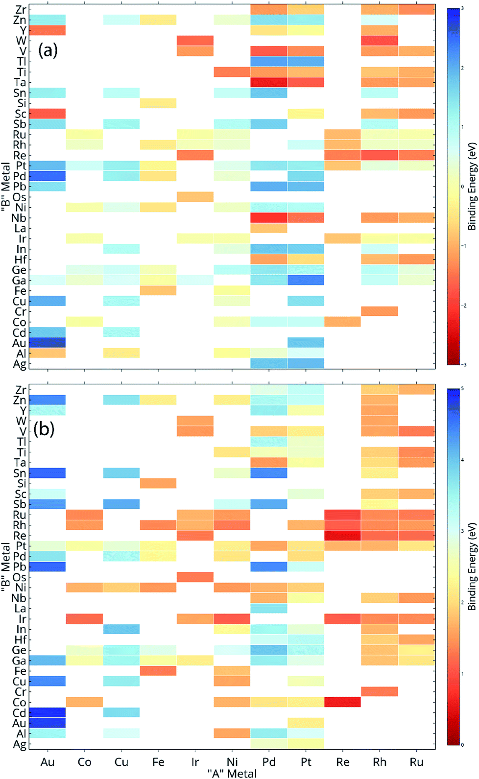

Fig. 2 The dataset used for the ML model for (a) oxygen and (b) carbon for AA terminated A₃B bimetallic alloys. Highlighted cells represent the “A” metal and “B” metal in the bimetallic alloy used in the dataset and the filled color represents the binding energy of oxygen/carbon taken from the CatApp database.

Fig. 3 The dataset used for the ML model for (a) oxygen and (b) carbon for AB terminated A₃B bimetallic alloys. Highlighted cells represent the “A” metal and “B” metal in the bimetallic alloy used in the dataset and the filled color represents the binding energy of oxygen/carbon taken from the CatApp database.

Thus, the prediction of binding energy is a complex non-linear problem. ML algorithms with their ability to learn complex non-linear interactions can therefore be used for predicting the binding energies of these bimetallic alloys.

Supervised learning is a type of ML task where the algorithm learns an inferred function from already labelled data. This inferred function is then used to predict the target value from new data. The “No Free Lunch” theorem in ML states that there is no one model that works best for all problems.⁶⁶ Hence, it is always advisable to try multiple ML algorithms to identify which model works best for a particular problem. A number of widely used ML algorithms were evaluated which can be classified as linear models, distance based models, support vector machines, tree based ensemble algorithms and neural networks.

For the prediction of oxygen binding energies on AA terminated A₃B bimetallic alloys, all models were initially tested by giving all 27 features as input. The optimum hyperparameters are obtained by using grid search with 10-fold cross validation for each algorithm as given in Table 2. Mean training and testing errors for each algorithm (for tuned hyperparameter values) are also shown in Table 2, along with the minimum and maximum errors for 100 trials. In each of these 100 trails, the data are split randomly into train and test data. The model is built on the training data and training error is evaluated on the same training data while the test error is evaluated on the testing data. The RMSE errors in eV for all the algorithms tested are shown in Fig. 4 and listed in Table 2.

Table 2 Optimum hyperparameters evaluated for each ML algorithm along with training and test errors for predicting oxygen binding energies for A₃B bimetallic alloys

ML algorithm	Tuned hyperparameter value	Train error mean (min, max)	Test error mean (min, max)
Linear regression	Non-parametric	0.43 (0.37, 0.46)	0.55 (0.43, 0.75)
Ridge regression	Alpha = [0.5]	0.44 (0.39, 0.48)	0.53 (0.36, 0.69)
K-nearest regression	n_neighbors = 5, weights = ‘distance’	0 (0, 0)	0.54 (0.35, 0.77)
Support vector regression	Kernel = [‘rbf’], c = [1000], gamma = [0.001]	0.23 (0.17, 0.26)	0.34 (0.24, 0.53)
Random forest regression	n_estimators = [400], max_depth = [6]	0.16 (0.13, 0.18)	0.35 (0.22, 0.52)
Extra tree regression	n_estimators = [100], max_depth = [6]	0.14 (0.10, 0.17)	0.32 (0.18, 0.47)
Gradient boosting regression	n_estimators = [400], max_depth = [3], learning_rate = [0.3]	0.003 (0.003, 0.003)	0.31 (0.2, 0.44)
Artificial neural network	Activation = [Relu], loss = [mean_squared_error], optimizer = [sgd]	0.19 (0.14, 0.23)	0.39 (0.25, 0.54)

---

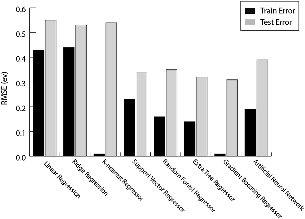Fig. 4 The train error and test error for the evaluated ML algorithms for predicting oxygen binding energies on A₃B bimetallic alloys.

Linear models tested include ordinary linear regression (OLR) and ridge regression. The OLR involves predicting the target variable as a linear function of the input features. It can be mathematically represented as

y(x, w) = w₀ + w₁x₁ + … + w_nx_n

They are easy to model and form the basis of many sophisticated ML algorithms.⁶⁷ Since the model is a linear function of input features, it only looks for linear relationships between the features and target value. As discussed before, the prediction of binding energy for bimetallic alloy is a non-linear problem and hence, a large test error of 0.55 eV and 0.53 eV is obtained for OLR and ridge regression respectively as given in Table 2.

The distance based model, k-nearest regression, is one of the simplest machine learning models. It is a non-parametric model where the principle is to predict a target by looking at the properties of its nearest neighbours in the training set.⁶⁸ Despite being simple and easy to interpret, these distance based models have been proven to be successful in various applications.⁶⁹ However, since the model computes distances every time a prediction needs to be made, it suffers from a poor run-time performance. Also, it is very sensitive to erroneous data and irrelevant features.⁶⁹ We obtained a large test error of 0.54 eV (Fig. 4 and Table 2) for the prediction of oxygen binding energies proving that distance based models do not work well for this problem.

Support Vector Regression (SVR) is a ML algorithm that uses high dimensional feature space to predict functions using a set of support vectors. Instead of minimising the training error during learning, it minimises the generalisation error.⁶⁹ It has been applied successfully to various problems like optical character recognition (OCR) and time series prediction.⁶⁹ A similar ML algorithm, Kernel Ridge Regression (KRR), is used for high-throughput screening of transition metal based organometallic catalysts for Suzuki cross-coupling reactions between alkyl substituted ethylene and vinyl bromide by Meyer et al.⁷⁰ The author studied >2500 organometallic complexes (6 different transition metals and 91 different ligands) and found 557 catalysts to satisfy the set criteria of the descriptor (reaction energy for the oxidative addition of vinyl bromide to the organometallic catalyst) within the range between −1.39 and −1.0 eV. The drawbacks of SVR include a high algorithmic complexity and extensive memory requirements,⁶⁹ whereas KKR is known for non-sparse solutions, leading to scalability problems for large data sets.^71,72 The RMSE error observed for SVR is 0.34 eV (Table 2), which is much better as compared to linear as well as distance based models.

The ensemble based algorithms used include Extra Tree Regression (ETR), Random Forest Regression (RFR) and Gradient Boosting Regression (GBR). The underlying goal of all the ensemble algorithms is to combine predictions from several weak estimators to construct a strong estimator. These algorithms differ in how they construct a number of decision trees to eventually build an ensemble. RFR builds ensembles of decision trees where each tree is built on a random selection of examples from the training data. Additionally, RFR adds randomness while constructing these trees. Instead of choosing the most important feature while splitting a node, it chooses the most important feature from a random sample of features.⁷³ ETR adds an extra layer of randomness to RFR.⁷⁴ The final prediction for a new input is made by averaging the predictions by each of the trees in the ensemble for both the algorithms. These decision tree based ensemble methods can capture linear as well as non-linear complex relationships⁷³ and thus RMSE error values observed for ETR and RFR are 0.32 eV and 0.35 eV respectively (Table 2). These tree based ML algorithms have been shown to be the best in predicting the binding energy of CH₄ related species (CH₃, CH₂, CH, C and H) over Cu based alloys.⁵²

Artificial Neural Networks (ANNs) have been inspired by the biological neural networks in the brain.⁷⁵ It consists of multiple interconnected nodes that are loosely modeled on neurons. Due to their ability to fit non-linear and complex data, their robustness to noise and adaptive learning, they have proven to be predictive in solving various complex real world problems.⁷⁶ However, they have received criticism because of their behaviour as a “black-box” – being hard to interpret and due to the requirement of high computational resources.⁷⁷ The observed RMSE error for ANNs is 0.39 eV (Table 2), which is higher as compared to SVR and tree based ensemble algorithms.

It can be seen from the error values that GBR performed better than any other model used in the study with a test error of 0.31 eV (Table 2) for predicting oxygen binding energy. A simple representation of GBR has been shown in Fig. 5. GBR is an ensemble algorithm where the decision trees are learned sequentially. Initially a weak learner (decision tree) is built and then the model is improved by adding to it another learner that is built on the error (also called residual) of the last learner. In general, the next learner tries to correct the errors of its predecessor.⁴⁹ The ensemble algorithms improve upon the biggest drawback of decision trees that is overfitting.^49,78 They produce models that are adaptable, easy to interpret and provide better prediction than many ML algorithms.⁵⁰ Also, the ability of GBR to fit non-linear relationships⁵⁰ results in its better prediction power for binding energy than many other ML algorithms. All such advantages of GBR coupled with the least RMSE error obtained in our case makes it the best choice for predicting binding energy. Thus, further analysis has been done using GBR only.

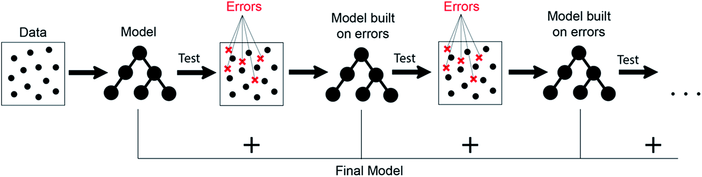Fig. 5 A simple representation of the gradient boosting decision tree algorithm.

The RMSE calculated over 100 trials for GBR is comparable to the error in binding energy calculations via DFT (∼0.3 eV).^55,79,80 The training and testing errors are evaluated by increasing the number of trials from 100 to 200 and 300. In each trial, a random split of data into training and testing data is performed. The RMSE errors were observed to be consistent averaged over 200 trials and 300 trails. This proves that the accuracy of the model remains stable even when the number of trials is increased.

3.1.1 Analysis of the computational time. Traditionally, all the important heterogeneous catalysts are developed using large scale screening experiments, which require a trial and error approach to identify an optimum catalyst for a reaction.⁸¹ For example, Alwin Mittasch and co-workers conducted over 6500 experiments and screened about 2500 catalysts^82,83 before arriving at an Fe-based catalyst very similar to what is industrially used for ammonia synthesis. Computationally, Nørskov and co-workers^{4,9,21,81,84,85} have shown relevant descriptors that can be identified to describe the activity of a catalyst. There can be many variables that affect the kinetics of the reaction such as the energy of transition states or the intermediates, but generally these variables are highly correlated. Thus, one or two independent descriptors can be identified in each case that can be used to predict the catalytic activity.⁴ This descriptor based approach has helped the screening of catalysts for reactions such as methanation,⁸⁶ ammonia synthesis,^81,85 hydrogen evolution²¹ and oxygen reduction.⁸⁷ Such descriptors in terms of binding energy of adsorbates over catalysts have been identified for a number of reactions.⁸⁴

Experiments are generally performed to measure the binding energy using temperature programmed desorption (TPD) and adsorption isotherms. More advanced and accurate experiments are now performed to measure binding energies using single crystal surfaces, which are well adapted in the work of Somorjai,⁸⁸ Ertl^89,90 Masel,⁹¹ King⁹² and Campbell.⁹³ However, all of them are time consuming and DFT calculations certainly help in speeding up the process. In this regard, a significant advantage of using ML over DFT calculations and tedious experiments is obtained in the reduction of both computational time and resources for the estimation of the binding energies of species on a catalyst surface. The average computational time taken for the calculation of a 4 × 4 (111) surface having 64 metal atoms is 2100 s with 8 CPUs (2.5 GHz/12-Core with 62 GB RAM), whereas the time taken for the calculation of systems with adsorbates is on average 4000 s. The time taken for the calculation of gas-phase CH₄, H₂O and H₂ is in the range of ∼100 s. In summary, on an average, the total computational time taken for single adsorption energy calculation is in the range of 6000 s or 100 min on 8 high performance CPUs. Meanwhile, the prediction of one adsorption energy value using GBR (after the model is built) is 0.0006 seconds on a dual-core laptop. Even when the complete computational time of the process is calculated, which includes the time taken for hyperparameter optimisation and then the time to calculate the test error for 100 random splits of test/train data, it takes about 480 seconds or 8 minutes on a dual-core laptop for the GBR model built for predicting oxygen binding on the dataset of A₃B bimetallic alloys. Thus, even if we start to build a new ML model for a completely new dataset, ML models would save a great amount of time and resource.

3.1.2 Feature importance for GBR prediction. Adsorbate interactions with a transition metal catalyst surface are suggested to occur via the molecular level interactions of the metal d-band and the molecular orbitals of the adsorbates.^4,5 The transition metal d-band itself contains features such as the d-band center, skewness, kurtosis etc. which are important descriptors of adsorbate binding energies. Most applicable surface science theories propagated by Nørskov and co-workers have simplified molecular level explanations of adsorbate–metal interaction with a desire to come up with simple descriptors such as the center of the d-band of the transition metal surface.^4,5 However, such simplistic descriptions often ignore the richness of surface–adsorbate interactions where the individual physical properties of the surface metals such as the group, period, atomic number, atomic mass, atomic radius, electronegativity, melting point, boiling point, density, heat of fusion, ionization energy and surface energy play an important role. The d-band theory has also shown disagreement with experimental results for a number of systems.^94–96 In a recent study by Bhattacharjee et al.,⁹⁷ a modified two-centered d-band model was proposed, where the two spin states (up and down spin) are considered separately. This is demonstrated to be better in predicting the binding energy for magnetic transition metals. Nonetheless, artificial neural networks have been shown to be efficient in predicting the binding energy of CO and OH over bimetallic alloys using the electronic d-band properties of bimetallic alloys as features.^26,27 However, the use of these electronic properties, which in turn need to be calculated via DFT, limits the usage of features for prediction.

Machine learning has also been used to predict the binding energy of CH₄ related species over Cu-based bimetallic alloys.⁵² The features used in the study were the physical properties of the other metal in the Cu-based alloy. The use of physical properties that are readily available in the literature makes this model much more interpretable and universal. Moreover, it facilitates the rapid discovery of new alloys as the features of every alloy are readily available. We build upon these features (which include the group, period, atomic number, atomic mass, atomic radius, electronegativity, melting point, boiling point, density, heat of fusion, ionization energy and surface energy of the catalyst elements) and extend it to all bimetallic alloys of the type A₃B, thus building a universal model which can be used to predict the binding energy of oxygen and carbon over any bimetallic alloy of the form A₃B. Additionally, features like the d-band center, Pauling electronegativity and work function have been used to describe the A element as used by Xin et al. in their work.^26,27 The relevance of such features is further consolidated by using them to predict the binding energy of oxygen and carbon over single atom alloys with the example of Cu-based SAAs. For industrial applications, bimetallic alloys are more appealing than SAAs as SAAs require sophisticated synthesis methods and current industrial bulk synthesis methods are not adequate to produce stable SAAs.^98,99

In addition, a separate analysis is performed to remove the least important features from the model so as to find the test error. On removing the features, the error is observed to increase, suggesting that the set of 27 features used collectively predicts the adsorption energy better. For oxygen binding energy prediction for AA terminated alloys, the test error obtained with the model using 27 features is 0.31 eV. For a model built with only the top 25 features, the test error is 0.32 eV, and for a model built with the top 20 and top 15 features, the test error is increased to 0.33 eV. This is tabulated in ESI Table SI-1.†

3.2 AA terminated A₃B bimetallic alloy

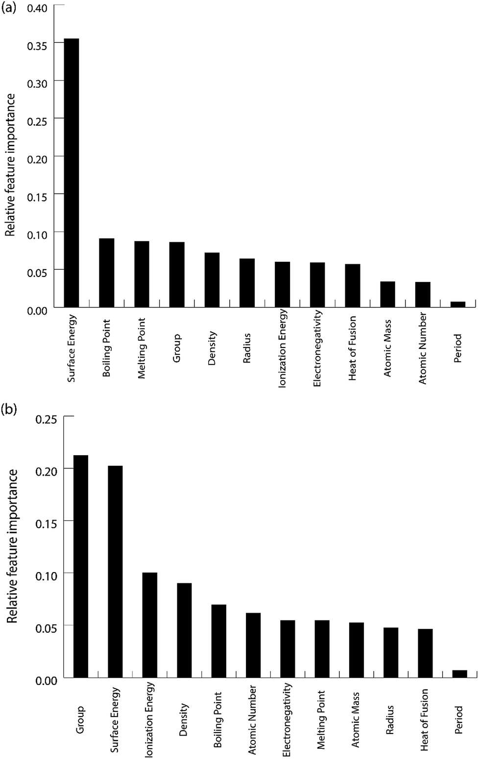
For the purpose of predicting the oxygen binding energy of AA terminated A₃B bimetallic alloys, a total of 27 features were used to describe each bimetallic alloy. The correlation matrix for oxygen binding energy with the individual features of “A” metal and “B” metal of A₃B bimetallic alloys is shown in Fig. 6(a) and (b). The “good” features are generally those that are not correlated with the other features and at the same time are highly correlated with the target variable.¹⁰⁰ The correlation plot shows that there may be a need for variable selection in order to obtain the best set of predictors. Each time a GBR model is trained, a feature importance matrix can be obtained that gives the relative importance of a feature with respect to other features for that model. The feature importance of a variable is measured based on two measures: the number of times it is used for splitting a node in the decision tree and the improvement in the model due to that split. This is averaged over all the trees in the model to calculate the final feature importance.⁷⁷ Surface energy has been shown to be a good descriptor of the catalytic activity of 15 different alloys in a previous study.¹⁰¹ Also, Takigawa et al. found surface energy as the most important feature in the ML prediction of the binding energies of C and CH over Cu based alloys.⁵² This is reiterated in our results where the surface energy of the B metal in the AA terminated A₃B alloy is the most important feature. Fig. 7(a) shows the feature importance for all features in the GBR model for the oxygen binding energy averaged out over 100 trials. We observe that the most important features belong to the dopant (B element) rather than the element that forms the matrix (A element) in the bimetallic alloy. Along with the surface energy, other important features for prediction are the ionization energy, electronegativity, density and heat of fusion of the dopant.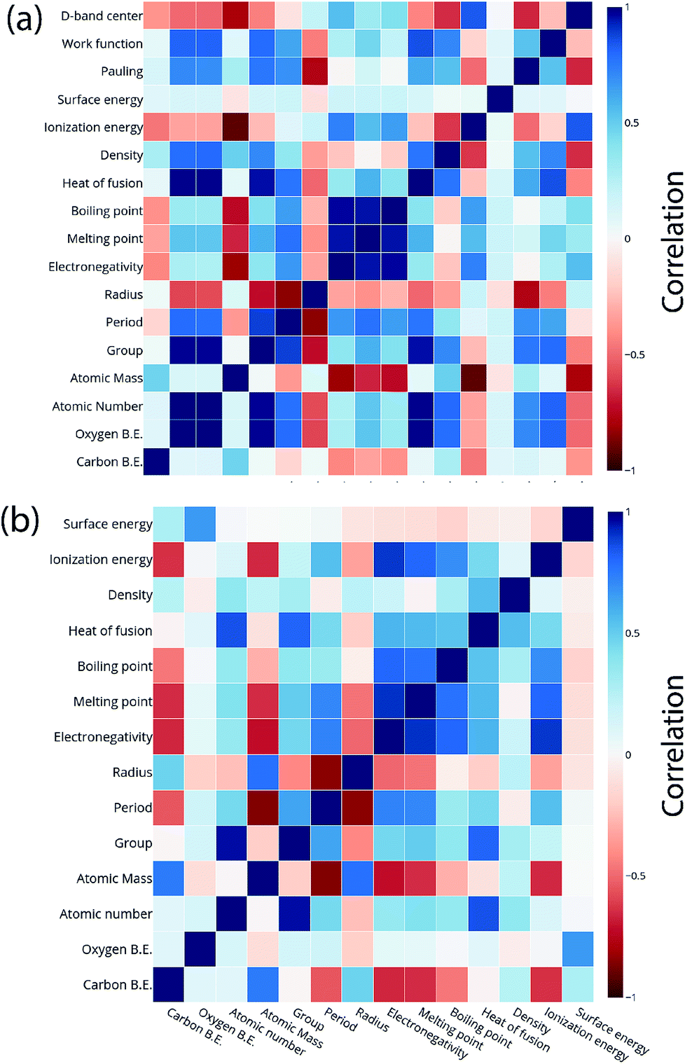

Fig. 6 Correlation plot for oxygen and carbon binding energy with the features of the (a) “A” metal and (b) “B” metal in the AA terminated A₃B bimetallic alloy (211) surface.

Fig. 7 Relative feature importance for the GBR model for predicting (a) oxygen and (b) carbon binding energies for the AA terminated A₃B bimetallic alloy (211) surface.

In order to optimize the ratio of test/train data split, additional analysis is performed to measure the RMSE of the model for test/train split ratios of 15/85, 20/80, 25/75, 30/70, and 50/50. The errors obtained in the above-mentioned cases are tabulated in Table 3. The test error increases as the ratio of test/train data is increased. As this ratio is increased, the amount of data available for training the model decreases. This resulted in the reduction of the accuracy of the model. Thus, it can be seen that the ML model improves with the availability of more training data. This also indicates that if we include more train data in our model, it should further decrease the RMSE error obtained. This increase in data could be achieved either by adding more number of alloys or including more relevant features for each alloy. The deviation of the predicted values from DFT calculated values for GBR for different ratios of test/train data is presented in Fig. 8.

Table 3 Effect on training and testing errors with the change of the test/train data ratio for the GBR model for predicting the binding energy of oxygen on the AA terminated A₃B bimetallic alloy (211) surface

Test/train split	Train error	Test error
15%/85%	0.0003	0.31
20%/80%	0.0003	0.31
25%/75%	0.0003	0.33
30%/70%	0.0003	0.35
50%/50%	0.0003	0.4

---

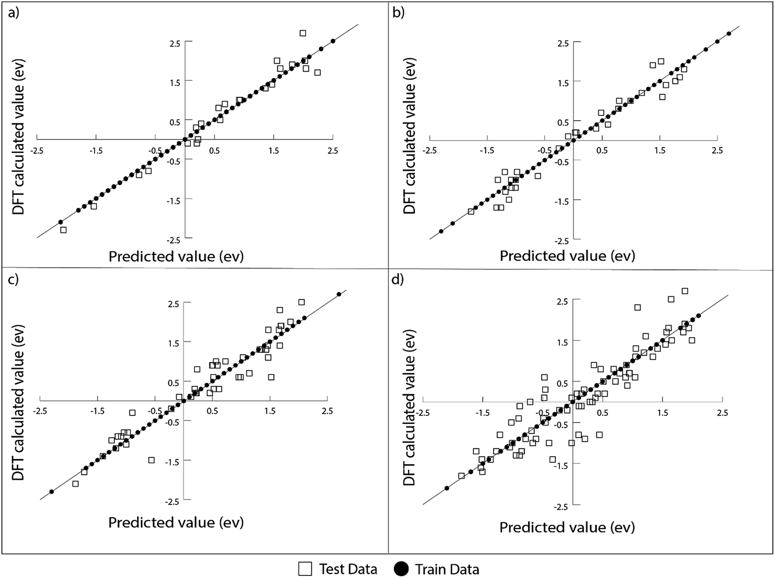Fig. 8 The deviation of DFT calculated oxygen binding energy from that predicted using the GBR model for the AA terminated A₃B bimetallic alloy for (a) a test/train ratio of 15/85, (b) a test/train ratio of 20/80, (c) a test/train ratio of 30/70 and (d) a test/train ratio of 50/50.

Another ML model was built to predict carbon binding energies for the AA terminated A₃B bimetallic alloys. Since we have established the relevance of GBR in predicting the binding energy of oxygen, only a GBR model was fitted for this prediction. In the data, instead of the oxygen binding energy, the carbon binding energy of AA terminated A₃B alloys was the target variable and the rest of the input features remained the same. Again, the optimum hyperparameters were obtained using grid search with a 10-fold cross validation in Scikit-learn. The test error for the optimized model averaged over 100 trials was found to be 0.34 eV. In each of these trials, the test and train data were chosen randomly. This proves that the GBR ML model can be effectively used to predict carbon binding energies for these bimetallic alloys with accuracies equivalent to that of DFT calculations. The deviation of the predicted values from DFT calculated values for GBR for different ratios of test/train data can be seen in Fig. SI-3† and the error obtained for different ratios of test/train splits are available in Table SI-2.† The features used were the same as those used for oxygen binding energy calculation. The correlation matrix of features of “A” metal and “B” metal for A₃B bimetallic alloys with the carbon binding energy can be seen in Fig. 6(a) and (b). The feature importance of this model was again calculated and is presented in Fig. 7(b). It can be seen that the top features for predicting the carbon binding energy remain almost similar to those for predicting oxygen binding energy. The surface energy of the dopant is still the most important feature followed by ionization energy and density. The fact that the most important features remain almost similar shows that these physical features are highly correlated with the binding energy. Moreover, the ML model is able to identify this correlation and predict the binding energies for both carbon and oxygen over AA terminated A₃B bimetallic alloys.

3.3 AB terminated A₃B bimetallic alloys

In order to demonstrate the ability of ML to predict the binding energies of bimetallic alloys for different surface configurations, we built a GBR model to predict the binding energies of oxygen and carbon for AB terminating A₃B bimetallic alloys as well. The same dataset of 151 A₃B bimetallic alloys is used; however, the target values are the binding energies of oxygen and carbon calculated over AB terminated alloys. The same procedure to build the GBR model was used as described before and the RMSE test error for oxygen and carbon binding energy for AB terminated bimetallic alloys are 0.38 eV and 0.35 eV, respectively. The deviation of the predicted values from DFT calculated values for oxygen binding energy and carbon binding energy for different ratios of test/train data can be seen in Fig. SI-4 and SI-5† respectively, whereas the respective errors obtained for the splits are tabulated in Tables SI-3 and SI-4.† This again represents that with the increase in train data, the ML algorithm predicts better. The feature importance for oxygen and carbon binding energy in the GBR model is calculated and presented in Fig. 9(a) and (b), respectively. However, in contrast to the feature importance obtained for the case of AA terminated alloys, the surface energies of both the dopant (B element) and the matrix (A element) are the most important features for both oxygen and carbon binding energy prediction. The other important features remain the same as for AA terminated surfaces and include the electronegativity, ionization energy, density and heat of fusion of the B element in the A₃B alloy.

Fig. 9 Relative feature importance for the GBR model for predicting (a) oxygen and (b) carbon binding energies for the AB terminated A₃B bimetallic alloy (211) surface.

Three most common features with high importance for binding energy over transition metal surfaces are surface energy, ionization energy and electronegativity. Surface energies are related to the degree of coordinative unsaturation of the surface metal atoms. In general, a system with higher surface energy is indicative of a surface with higher reactivity. The ionization potential and electron affinity are related to the ease of electron transfer between the surface metal atoms and the adsorbate and known to be important parameters for chemical bonding. Though ML models are mostly used as a black-box model driven by data, an added advantage of GBR feature importance is the underlying physics that is captured from this model.

3.4 Single atom alloys

We calculated the data for the binding energy of oxygen and carbon over Cu-based SAAs via DFT in order to demonstrate the reliability of ML model prediction for SAAs as well. The 27 metals used for forming the single atom alloys have been highlighted in the periodic table, according to the oxygen and carbon binding energy as shown in Fig. 10(a) and (b), respectively. For oxygen binding energies, large negative values are observed for early transition metals (−1.71 eV for W). As we move from left to right in the periodic table, the binding energy moves towards the positive scale peaking at Pt (1.77 eV) and Pd (1.68 eV). A somewhat similar trend is also observed for carbon binding energy values although the binding energy values are all positive.

Fig. 10 Elements used as single atoms in the Cu-based SAA in the dataset. The highlighted color represents the binding energy of (a) oxygen and (b) carbon on the respective SAA as calculated from DFT calculations.

All the models are tested with 12 features as input which include the physical properties (group, period, atomic number, atomic mass, atomic radius, electronegativity, melting point, boiling point, density, heat of fusion, ionization energy and surface energy) of single atoms in the alloy. The correlation matrix of features of “B” metal for Cu-based SAAs for the carbon and oxygen binding energy can be seen in Fig. 11. The features describing Cu are not included as they would remain constant for all the alloys used in the model. Again, a similar procedure is followed to get the optimized GBR models as mentioned for the case of A₃B bimetallic alloys. A set of hyperparameters are tested using 10-fold cross validation in order to obtain the best hyperparameters for the GBR model. The test error for the optimized models averaged over 100 trials for oxygen binding energies and the carbon binding energies are 0.36 eV and 0.37 eV respectively. This result again shows the effectiveness of the GBR model for the prediction of binding energies. The deviation of the DFT calculated values from the predicted values for different test/train ratios for predicting oxygen and carbon binding energies can be seen in Fig. SI-6 and SI-7† respectively. Errors obtained at the above different test/train ratios are tabulated in Tables SI-5 and SI-6† for oxygen and carbon binding energies over SAAs respectively. This again illustrates that increasing the train data improves the prediction of the GBR model.

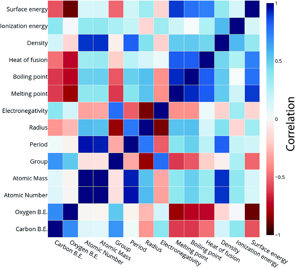Fig. 11 Correlation plot for oxygen and carbon binding energy with the features of the single atom metal in the Cu-based SAA.

The feature importance for the optimized models for the prediction of oxygen and carbon binding energies is shown in Fig. 12(a) and (b) respectively. The most important feature for the prediction of carbon binding energy is still the surface energy of the element. The rest of the features have almost similar relative importance. This again shows the high correlation between surface energy and the binding energy; and the adequacy of the ML model to identify this correlation for prediction. However, for the prediction of oxygen binding energies, both the group and surface energy of the single atom have similar importance. The importance of the group in the prediction is also observed in the study by Takigawa et al.,⁵² where it is the most important feature for predicting the binding energies of H and CH₂ over Cu-based alloys.

Fig. 12 Relative feature importance for the GBR model for predicting (a) carbon and (b) oxygen binding energies for the Cu-based SAA.

3.5 In silico screening using ab initio microkinetic modelling

The binding energy of alloys obtained from ML is further verified by microkinetic modeling. This was implemented using the CatMAP module,⁶ wherein the reaction energetics are derived for DFT based alloy energies as well as those acquired from ML. The MKM is evaluated for two reactions for which previously alloy catalyst search has been undertaken. The two reactions are ethanol decomposition¹³ and NODH of ethanol.¹⁵ A similar approach has been employed by Xin et al.^26,27 and Ullisi et al.^39,40 using ANN based ML algorithms. The models are constructed using d-band features for the alloys, along with a MKM to predict catalytic rates for bimetallic alloys for various reactions like CO₂ reduction, the OER, etc.

Fig. 13 depicts the turnover of the products of reaction for ethanol decomposition over DFT as well as ML based alloy binding energies. The reaction conditions are considered to be T = 573 K and P = 2 bar with an inlet stream ratio of 1 : 1 for ethanol and hydrogen. Ethane is formed upon C–O scission of ethanol, whereas methane is the C–C scission product as shown in Fig. 13(a) and (b) respectively. It can be inferred from Fig. 13 that the activity trend over the alloys remains the same for DFT and ML based alloy energies. The activity trend for DFT based alloy energetics is Co₃Ru ∼ Ni₃Fe ∼ Co₃Ni ∼ Co₃Fe > Ni₃Cu > Ni₃Pt > Ni₃Rh,¹³ whereas that based on ML alloy energetics is Co₃Ru > Ni₃Fe ∼ Co₃Ni ∼ Co₃Fe > Ni₃Cu ∼ Ni₃Pt ∼ Ni₃Rh. The turnover of the C–O scission product (ethane) over the alloys is given in Table 4. For Co₃Ru, Ni₃Rh, and Ni₃Pt, the calculated TOF remains the same for both the DFT and ML energetics. However, for the rest of the alloys, the TOFs are underpredicted for energies obtained from ML by an order of magnitude. An error bar of 0.3 eV is considered for C and O binding energies on the metals and metal alloys as this is comparable to the error found in the ML model tested in the study.

Fig. 13 Comparison of TOFs of ethanol decomposition to produce (a) ethane and (b) methane on Co and Ni based bimetallic alloys as obtained from DFT (circle) and ML (square). Error bar = 0.3 eV.

Table 4 TOF of ethane production from ethanol decomposition over Ni and Co based bimetallic alloys obtained using DFT and ML calculated binding energies

Alloy	TOF [DFT]	TOF [ML]
Ni3Fe	10^−3 s^−1	10^−4 s^−1
Ni3Rh	10^−5 s^−1	10^−5 s^−1
Ni3Cu	10^−4 s^−1	10^−5 s^−1
Ni3Pt	10^−5 s^−1	10^−5 s^−1
Co3Fe	10^−3 s^−1	10^−4 s^−1
Co3Ni	10^−3 s^−1	10^−4 s^−1
Co3Ru	10^−3 s^−1	10^−3 s^−1

---

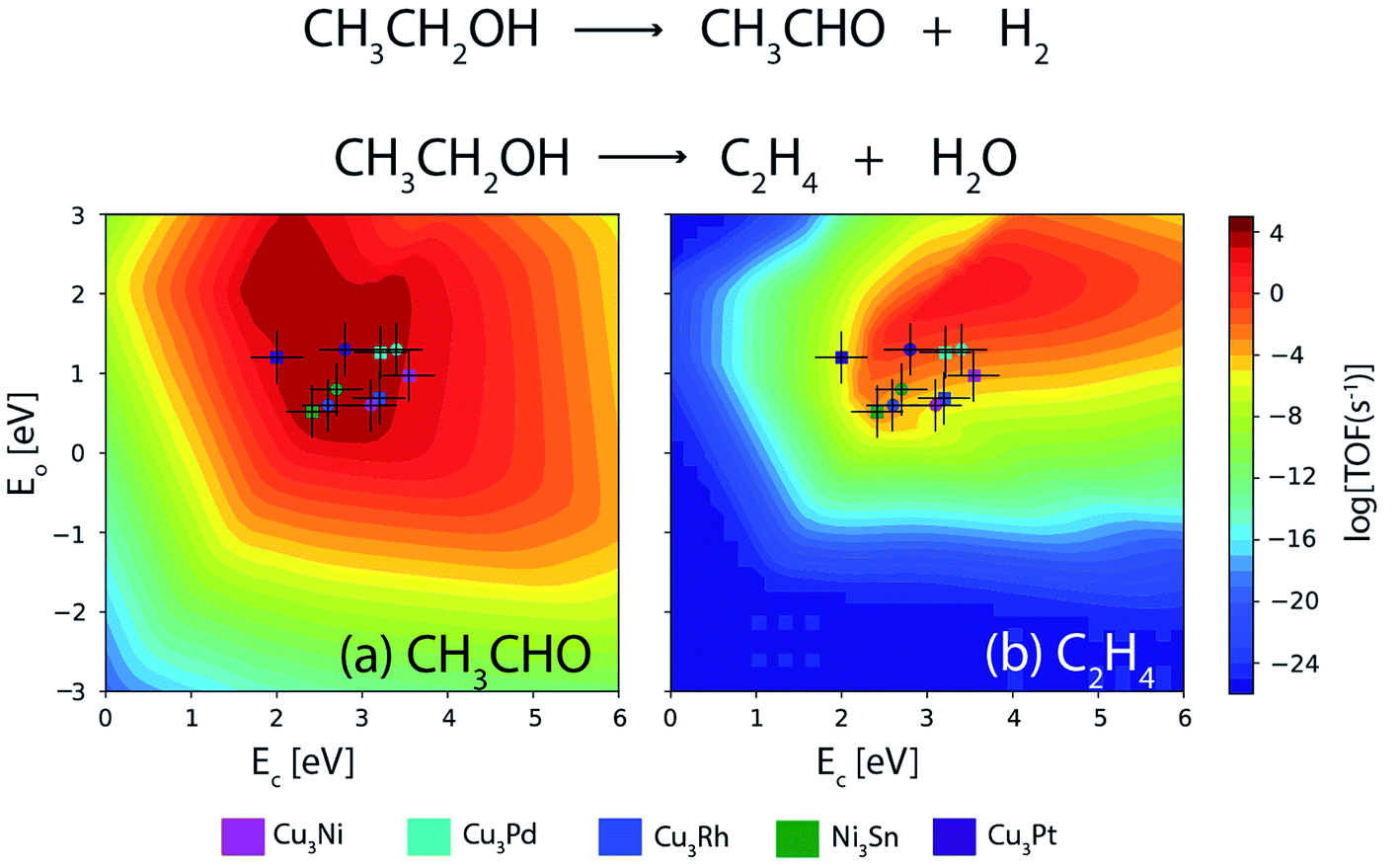
Furthermore, a similar comparison study is conducted for the NODH of ethanol at 473 K and an initial conversion of 10%. Fig. 14(a) and (b) show the volcano plots for the reaction products: acetaldehyde and ethylene over the alloys as well as transition metals for descriptor energies obtained from DFT¹⁵ and ML respectively. The TOFs of acetaldehyde over the alloys are listed in Table 5. For Ni₃Sn, Cu₃Rh and Cu₃Pd, the TOF remains the same for both DFT and ML; however for Cu₃Ni and Cu₃Pt, a difference of an order of magnitude is observed in the TOF between the two methods. Overall, it can be concluded that the obtained trend in TOFs on alloys is similar and the difference in individual TOF values between ML and DFT predictions is not more than an order of magnitude. Therefore, increasing the input alloy data set of DFT calculations for ML models can thereby enhance the accuracy of ML. ML models in combination of MKM gives direct access to an in silico catalyst screening process, where GBR based ML models can be applied in tandem with already existing database and MKM models to screen potential bimetallic alloy or single atom alloy catalyst candidates faster than conventional DFT based methods, without compromising the accuracy.

Fig. 14 Comparison of TOFs for the NODH of ethanol to produce (a) acetaldehyde and (b) ethylene on bimetallic alloys as obtained from DFT (circle) and ML (square). Error bar = 0.3 eV.

Table 5 TOFs of acetaldehyde production from NODH of ethanol over bimetallic alloys obtained using DFT and ML calculated binding energies

Alloy	TOF [DFT]	TOF [ML]
Ni3Sn	10^4 s^−1	10^4 s^−1
Cu3Rh	10^4 s^−1	10^4 s^−1
Cu3Ni	10^4 s^−1	10^3 s^−1
Cu3Pt	10^4 s^−1	10^3 s^−1
Cu3Pd	10^4 s^−1	10^4 s^−1

---

4. Conclusion

ML models are developed to predict the binding energy of oxygen and carbon over bimetallic and SAAs. Among all the ML models studied, the GBR model is observed to be superior in giving significantly reduced errors. The model is enriched by incorporating several features of the catalyst surface, which include the periodic properties of the elements and many other electronic properties. The ML model, therefore, contains more descriptive information about adsorbate–surface interactions as compared to commonly applied simplified surface science theories based on the d-band center of the transition metal catalyst. For example, in predicting the binding energies of carbon and oxygen atoms on all of the alloys studied, the surface energy, electronegativity, ionization energy, density and heat of fusion of the alloying metals are considered to be the most significant features in exercising maximum influence on adsorption. However, as an exception, in the case of single atom alloys, the periodic group of single metal atoms, alloyed on the surface of a less reactive metal, is observed to be the most important feature. The GBR model built using readily available features of the participating metals can be applied to estimate the binding energies of important adsorbate species for both bimetallic alloys and SAAs, with good accuracy, making the approach more universal. These feature enabled molecular level insights further augment the the importance of the ML model as compared to computationally intensive DFT calculations or experiments required for the screening of catalyst materials. The applicability of the ML model in predicting the binding energies of metal alloys in an ab initio MKM is demonstrated for two different reactions of ethanol. In both the reactions, the ML model predicted TOFs similar to what was earlier obtained from DFT calculations. With the increase in the availability of alloy data from DFT calculations, ML models are expected to become more accurate. To sum up, the use of ML models will significantly reduce the time required for high throughput screening, with enriched and improvised understanding of the metal–adsorbate interactions.

Conflicts of interest

There are no conflicts to declare.

Acknowledgements

Financial support from the Department of Science and Technology, Government of India Grant, DST/TMD/MECSP/2KI7/07 to MAH is acknowledged. Computational resources of the High Performance Computing Facility at IIT Delhi are acknowledged. Authors would like to acknowledge Ankur Tomar for the cover illustration.

References

1. C. T. Campbell, ACS Catal., 2017, 7, 2770–2779.
2. C. Stegelmann, A. Andreasen and C. T. Campbell, J. Am. Chem. Soc., 2009, 131, 8077–8082.
3. C. A. Wolcott, A. J. Medford, F. Studt and C. T. Campbell, J. Catal., 2015, 330, 197–207.
4. J. K. Nørskov, F. Abild-Pedersen, F. Studt and T. Bligaard, Proc. Natl. Acad. Sci. U. S. A., 2011, 108, 937–943.
5. J. K. Nørskov, F. Studt, F. Abild-Pedersen and T. Bligaard, Fundamental concepts in heterogeneous catalysis, John Wiley & Sons, 2014.
6. A. J. Medford, C. Shi, M. J. Hoffmann, A. C. Lausche, S. R. Fitzgibbon, T. Bligaard and J. K. Nørskov, Catal. Lett., 2015, 145, 794–807.
7. L. C. Grabow, F. Studt, F. Abild-Pedersen, V. Petzold, J. Kleis, T. Bligaard and J. K. Nørskov, Angew. Chem., Int. Ed., 2011, 50, 4601–4605.
8. F. Studt, F. Abild-Pedersen, Q. Wu, A. D. Jensen, B. Temel, J.-D. Grunwaldt and J. K. Nørskov, J. Catal., 2012, 293, 51–60.
9. A. J. Medford, A. Vojvodic, J. S. Hummelshøj, J. Voss, F. Abild-Pedersen, F. Studt, T. Bligaard, A. Nilsson and J. K. Nørskov, J. Catal., 2015, 328, 36–42.
10. H. Falsig, J. Shen, T. S. Khan, W. Guo, G. Jones, S. Dahl and T. Bligaard, Top. Catal., 2014, 57, 80–88.
11. Y. Xu, A. C. Lausche, S. Wang, T. S. Khan, F. Abild-Pedersen and F. Studt, New J. Phys., 2013, 15, 125021.
12. A. C. Lausche, A. J. Medford, T. S. Khan, Y. Xu, T. Bligaard, F. Abild-Pedersen, J. K. Nørskov and F. Studt, J. Catal., 2013, 307, 275–282.
13. F. Jalid, T. S. Khan, F. Qayoom and M. A. Haider, J. Catal., 2017, 353, 265–273.
14. T. S. Khan, S. Hussain, U. Anjum and M. A. Haider, Electrochim. Acta, 2018, 281, 654–664.
15. T. S. Khan, F. Jalid and M. A. Haider, Top. Catal., 2018, 61, 1820–1831.
16. F. Abild-Pedersen, Catal. Today, 2016, 272, 6–13.
17. S. Wang, V. Petzold, V. Tripkovic, J. Kleis, J. G. Howalt, E. Skúlason, E. M. Fernández, B. Hvolbæk, G. Jones, A. Toftelund, H. Falsig, M. Björketun, F. Studt, F. Abild-Pedersen, J. Rossmeisl, J. K. Nørskov and T. Bligaard, Phys. Chem. Chem. Phys., 2011, 13, 20760.
18. S. Wang, V. Vorotnikov, J. E. Sutton and D. G. Vlachos, ACS Catal., 2014, 4, 604–612.
19. J. Greeley, Annu. Rev. Chem. Biomol. Eng., 2016, 7, 605–635.
20. J. S. Hummelshøj, F. Abild-Pedersen, F. Studt, T. Bligaard and J. K. Nørskov, Angew. Chem., Int. Ed., 2012, 51, 272–274.
21. J. K. Nørskov, T. Bligaard, J. Rossmeisl and C. H. Christensen, Nat. Chem., 2009, 1, 37.
22. M. Neurock, J. Catal., 2003, 216, 73–88.
23. M. K. Sabbe, M.-F. Reyniers and K. Reuter, Catal. Sci. Technol., 2012, 2, 2010–2024.
24. S. Curtarolo, G. L. W. Hart, M. B. Nardelli, N. Mingo, S. Sanvito and O. Levy, Nat. Mater., 2013, 12, 191.
25. J. Greeley and N. M. Markovic, Energy Environ. Sci., 2012, 5, 9246–9256.
26. Z. Li, S. Wang, W. S. Chin, L. E. Achenie and H. Xin, J. Mater. Chem. A, 2017, 5, 24131–24138.
27. Z. Li, X. Ma and H. Xin, Catal. Today, 2017, 280, 232–238.
28. J. E. Sutton and D. G. Vlachos, Chem. Eng. Sci., 2015, 121, 190–199.
29. A. Jain and T. Bligaard, Phys. Rev. B, 2018, 98, 214112.
30. M. M. Montemore and J. W. Medlin, Catal. Sci. Technol., 2014, 4, 3748–3761.
31. E. M. Fernández, P. G. Moses, A. Toftelund, H. A. Hansen, J. I. Martínez, F. Abild-pedersen, J. Kleis, B. Hinnemann, J. Rossmeisl, T. Bligaard and J. K. Nørskov, Angew. Chem., Int. Ed., 2008, 47, 4683–4686.
32. F. Abild-Pedersen, J. Greeley, F. Studt, J. Rossmeisl, T. R. Munter, P. G. Moses, E. Skúlason, T. Bligaard and J. K. Nørskov, Phys. Rev. Lett., 2007, 99, 16105.
33. G. Jones, F. Studt, F. Abild-Pedersen, J. K. Nørskov and T. Bligaard, Chem. Eng. Sci., 2011, 66, 6318–6323.
34. J. S. Yoo, T. S. Khan, F. Abild-Pedersen, J. K. Nørskov and F. Studt, Chem. Commun., 2015, 51, 2621–2624.
35. S. Wang, B. Temel, J. Shen, G. Jones, L. C. Grabow, F. Studt, T. Bligaard, F. A. Claus and H. C. Jens, Catal. Lett., 2011, 141, 370–373.
36. A. Khorshidi and A. Peterson, Comput. Phys. Commun., 2016, 207, 310–324.
37. K. Saravanan, J. R. Kitchin, O. A. Von Lilienfeld and J. A. Keith, J. Phys. Chem. C, 2017, 8, 5002–5007.
38. B. R. Goldsmith, J. Esterhuizen, J. Liu, C. J. Bartel and C. Sutton, AIChE J., 2018, 64, 2311–2323.
39. S. Back, K. Tran and Z. W. Ulissi, ACS Catal., 2019, 9, 7651–7659.
40. Z. W. Ulissi, M. T. Tang, J. Xiao, X. Liu, D. A. Torelli, M. Karamad, K. Cummins, C. Hahn, N. S. Lewis, T. F. Jaramillo, K. Chan and J. K. Nørskov, ACS Catal., 2017, 7, 6600–6608.
41. S. Back, J. Yoon, N. Tian, W. Zhong, K. Tran and Z. W. Ulissi, J. Phys. Chem. Lett., 2019, 10, 4401–4408.
42. K. Tran, A. Palizhati, S. Back and Z. W. Ulissi, J. Chem. Inf. Model., 2018, 58, 2392–2400.
43. Z. Li, S. Wang and H. Xin, Nat. Catal., 2018, 1, 10–12.
44. A. Nandy, J. Zhu, J. P. Janet, C. Duan, R. B. Getman and H. J. Kulik, ACS Catal., 2019, 9, 8243–8255.
45. J. P. Janet, L. Chan and H. J. Kulik, J. Phys. Chem. Lett., 2018, 9, 1064–1071.
46. C. Duan, J. P. Janet, F. Liu, A. Nandy and H. J. Kulik, J. Chem. Theory Comput., 2019, 15, 2331–2345.
47. H. J. Kulik, Wiley Interdiscip. Rev.: Comput. Mol. Sci., 2019, e1439.
48. J. Schmidhuber, Neural Networks, 2015, 61, 85–117.
49. J. H. Friedman, Computational Statistics & Data Analysis, 2002, 38, 367–378.
50. J. Ye, J.-H. Chow, J. Chen and Z. Zheng, in Proceedings of the 18th ACM Conference on Information and Knowledge Management, ACM, New York, NY, USA, 2009, pp. 2061–2064.
51. Y. Freund and R. E. Schapire, J. Jpn. Soc. Artif. Intell., 1999, 14, 771–780.
52. T. Toyao, K. Suzuki, S. Kikuchi, S. Takakusagi, K. Shimizu and I. Takigawa, J. Phys. Chem. C, 2018, 122, 8315–8326.
53. G. Kresse and J. Furthmuller, Comput. Mater. Sci., 1996, 6, 15–50.
54. D. Vanderbilt, Phys. Rev. B: Condens. Matter Mater. Phys., 1990, 41, 7892–7895.
55. B. Hammer, L. B. Hansen and J. K. Nørskov, Phys. Rev. B: Condens. Matter Mater. Phys., 1999, 59, 7413–7421.
56. H. J. Monkhorst and J. D. Pack, Phys. Rev. B: Solid State, 1976, 13, 5188–5192.
57. R. Tran, Z. Xu, B. Radhakrishnan, D. Winston, W. Sun, K. A. Persson and S. P. Ong, Sci. Data, 2016, 3, 160080.
58. D. R. Lide, CRC Handbook of Chemistry and Physics, CRC Press, Boca Raton, FL, 84th edn, 2003.
59. B. Hammer and J. K. Nørskov, in Advances in Catalysis, Academic Press, 2000, vol. 45, pp. 71–129.
60. F. Pedregosa, G. Varoquaux, A. Gramfort, V. Michel, B. Thirion, O. Grisel, M. Blondel, P. Prettenhofer, R. Weiss, V. Dubourg, J. Vanderplas, A. Passos, D. Cournapeau, M. Brucher, M. Perrot and É. Duchesnay, J. Mach. Learn. Res., 2011, 12, 2825–2830.
61. F. Chollet, Keras, GitHub.
62. M. Abadi, P. Barham, J. Chen, Z. Chen, A. Davis, J. Dean, M. Devin, S. Ghemawat, G. Irving, M. Isard, M. Kudlur, J. Levenberg, R. Monga, S. Moore, D. G. Murray, B. Steiner, P. Tucker, V. Vasudevan, P. Warden, M. Wicke, Y. Yu and X. Zheng, in Proceedings of the 12th USENIX Conference on Operating Systems Design and Implementation, USENIX Association, Berkeley, CA, USA, 2016, pp. 265–283.
63. Q. V. Le, M. Ranzato, R. Monga, M. Devin, K. Chen, G. S. Corrado, J. Dean and A. Y. Ng, in Proceedings of the 29th International Conference on International Conference on Machine Learning, Omnipress, USA, 2012, pp. 507–514.
64. L. C. Grabow, Computational Catalyst Screening, The Royal Society of Chemistry, 1st edn, 2014.
65. M. T. Darby, M. Stamatakis, A. Michaelides and E. C. H. Sykes, J. Phys. Chem. Lett., 2018, 9, 5636–5646.
66. D. H. Wolpert, in Soft Computing and Industry: Recent Applications, ed. R. Roy, M. Köppen, S. Ovaska, T. Furuhashi and F. Hoffmann, Springer London, London, 2002, pp. 25–42.
67. N. M. Nasrabadi, J. Electron. Imaging, 2007, 16, 49901.
68. N. S. Altman, Am. Stat., 1992, 46, 175–185.
69. P. Cunningham, M. Cord and S. J. Delany, Supervised Learning, in Machine Learning Techniques for Multimedia, ed. M. Cord and P. Cunningham, Springer Berlin Heidelberg, Berlin, Heidelberg, 2008, pp. 21–49.
70. B. Meyer, B. Sawatlon, S. Heinen, O. A. Von Lilienfeld and C. Corminboeuf, Chem. Sci., 2018, 9, 7069–7077.
71. N. Krämer and M. L. Braun, in Proceedings of the 24th International Conference on Machine Learning, ACM, New York, NY, USA, 2007, pp. 441–448.
72. K. Hansen, F. Biegler, S. Fazli, M. Rupp, M. Sche, O. A. Von Lilienfeld, A. Tkatchenko and K. Mu, J. Chem. Theory Comput., 2013, 9, 3404–3419.
73. L. Breiman, Mach. Learn., 2001, 45, 5–32.
74. P. Geurts, D. Ernst and L. Wehenkel, Mach. Learn., 2006, 63, 3–42.
75. B. Yegnanarayana, Artificial neural networks, PHI Learning Pvt. Ltd., 2009.
76. I. A. Basheer and M. Hajmeer, J. Microbiol. Methods, 2000, 43, 3–31.
77. J. V. Tu, J. Clin. Epidemiol., 1996, 49, 1225–1231.
78. B. J. H. Friedman, Ann. Stat., 2001, 29, 1189–1232.
79. A. J. Medford, A. C. Lausche, F. Abild-Pedersen, B. Temel, N. C. Schjødt, J. K. Nørskov and F. Studt, Top. Catal., 2014, 57, 135–142.
80. A. J. Medford, J. Wellendorff, A. Vojvodic, F. Studt, F. Abild-Pedersen, K. W. Jacobsen, T. Bligaard and J. K. Nørskov, Science, 2014, 345, 197–200.
81. C. J. H. Jacobsen, S. Dahl, B. S. Clausen, S. Bahn, A. Logadottir and J. K. Nørskov, J. Am. Chem. Soc., 2001, 123, 8404–8405.
82. S. R. Tennison, Catalytic Ammonia Synthesis, Springer US, 1991.
83. A. Mittasch and W. Frankenburg, Adv. Catal., 1950, 2, 81–104.
84. T. Bligaard, J. K. Nørskov, S. Dahl, J. Matthiesen, C. H. Christensen and J. Sehested, J. Catal., 2004, 224, 206–217.
85. J. K. Honkala, A. Hellman, I. Remediakis, A. Logadottir, A. Carlsson, S. Dahl, C. H. Christensen and J. K. Nørskov, Science, 2005, 307, 555–558.
86. A. L. Kustov, A. M. Frey, K. E. Larsen, T. Johannessen, J. K. Nørskov and C. H. Christensen, Appl. Catal., A, 2007, 320, 98–104.
87. J. Greeley, I. E. L. Stephens, A. S. Bondarenko, T. P. Johansson, H. A. Hansen, T. F. Jaramillo, J. Rossmeisl, I. Chorkendorff and J. K. Nørskov, Nat. Chem., 2009, 1, 552.
88. G. A. Somorjai, Introduction to surface chemistry and catalysis, John Wiley & Sons, 2010.
89. C. T. Campbell, G. Ertl, H. Kuipers and J. Segner, J. Chem. Phys., 1980, 73, 5862–5873.
90. G. Ertl, Catal. Rev., 1980, 21, 201–223.
91. D. A. Kyser and R. I. Masel, Rev. Sci. Instrum., 1987, 58, 2141–2144.
92. C. E. Borroni-Bird, N. Al-Sarraf, S. Andersoon and D. A. King, Chem. Phys. Lett., 1991, 183, 516–520.
93. O. Lytken, W. Lew and C. T. Campbell, Chem. Soc. Rev., 2008, 37, 2172–2179.
94. M. T. Gorzkowski and A. Lewera, J. Phys. Chem. C, 2015, 119, 18389–18395.
95. H. Thirumalai and J. R. Kitchin, Top. Catal., 2018, 61, 462–474.
96. M. P. Hyman, B. T. Loveless and J. W. Medlin, Surf. Sci., 2007, 601, 5382–5393.
97. S. Bhattacharjee, U. V. Waghmare and S.-C. Lee, Sci. Rep., 2016, 6, 35916.
98. Y. Chen, S. Ji, C. Chen, Q. Peng, D. Wang and Y. Li, Joule, 2018, 2, 1242–1264.
99. A. Wang, J. Li and T. Zhang, Nat. Rev. Chem., 2018, 2, 65–81.
100. M. A. Hall and L. A. Smith, in Computer Science ’98 Proceedings of the 21st Australasian Computer Science Conference ACSC’98, Perth, 4-6 February, ed. C. McDonald, Springer, Conference held at Perth, 1998, pp. 181–191.
101. H. Zhuang, A. J. Tkalych and E. A. Carter, J. Phys. Chem. C, 2016, 120, 23698–23706.

---

Footnotes

† Electronic supplementary information (ESI) available. See DOI: 10.1039/c9ta07651d

‡ Equal contribution.

---