The influence of motility on bacterial accumulation in a microporous channel

Abstract

We study the transport of bacteria in a porous media modeled by a square channel containing one cylindrical obstacle via molecular dynamics simulations coupled to a lattice Boltzmann fluid. Our bacteria model is a rod-shaped rigid body which is propelled by a force-free mechanism. To account for the behavior of living bacteria, the model also incorporates a run-and-tumble process. The model bacteria are capable of hydrodynamically interacting with both of the channel walls and the obstacle. This enables the bacteria to get reoriented when experiencing a shear-flow. We demonstrate that this model is capable of reproducing the bacterial accumulation on the rear side of an obstacle, as has recently been experimentally observed by [G. L. Miño, et al., Adv. Microbiol., 2018, 8, 451] using E. coli bacteria. By systematically varying the external flow strength and the motility of the bacteria, we resolve the interplay between the local flow strength and the swimming characteristics that lead to the accumulation. Moreover, by changing the geometry of the channel, we also reveal the important role of the interactions between the bacteria and the confining walls for the accumulation process.

---

I. Introduction

A growing number of emergent technologies take advantage of bacteria metabolisms to provide novel, environmentally-friendly, and more efficient alternatives to classical physicochemical methods. This is, for example, the case in the fields of pollution reduction,^1,2 oil recovery^3–5 biocalcification for soil reinforcement,^6,7 or to heal cement cracks.^8,9 However, one of the problems researchers face when trying to optimize these processes is the limited understanding of the role that bacterial motility plays at the pore scale^10–14 and its coupling to local chemical gradients.¹⁵ Indeed, we now know that flagellated microorganisms such as E. coli, or sperm cells display a great variety of swimming behaviors like upstream motions,^16–18 drift trajectories on surfaces^19,20 or helicoidal trajectories in a flow.^21,22 These motions contribute significantly to the trapping of bacteria in pores as well as in determining their localization in a channeled flow²³ and their hydrodynamic dispersion.^14,24,25 One of the consequences is an enhanced attachment and colonization of surfaces^23,26–28 which influences the biofilm formation²⁹ and therefore the overall fluid flow.^29,30 The aim of this work is to elucidate the important role that motility and geometric confinement play at the pore scale for the accumulation of bacteria on surfaces in a complex geometry.

Analytical tractable models and simulations can help to understand the experimental observations by elucidating the microscopic physics at play. The majority of the bacteria models incorporate mechanical torques by idealizing the shape of the bacteria, i.e., simple forms like rods or prolate particles.^23,26,31,32 Despite the apparent simplicity of these models, they are able to capture the complex helicoidal trajectories of microswimmers in a Poiseuille flow,^22,23 the accumulation of bacteria on flat surfaces²³ or downstream obstacles.²⁶ These models, however, exclude any particle–particle and particle-surface interactions, do not take into account the influence of the bacteria on the fluid flow, and neglect any steric effects. To overcome these limitations, we propose a hybrid modeling approach that couples the lattice-Boltzmann (LB) method to molecular dynamics (MD).^33–39 Employing this method, we are able to reproduce trajectories of model bacteria in a porous medium in order to understand the mechanism of how bacteria interact with the surrounding fluid's movement and how they accumulate on surfaces.

Our model for a microporous environment consists of a cylindrical obstacle placed under a microfluidic flow, mimicking the experimental setup of ref. 40. This geometry has been chosen because it contains the basic ingredients found in porous media: solid surfaces, velocities that vary along the stream lines, and stagnant flow zones (regions of low velocities). The referred experimental article will also serve to validate our simulation approach. Our model for E. coli bacteria is based on the one proposed in ref. 41. Here we couple hundreds of these dipolar force-free swimmers to a lattice-Boltzmann fluid to capture the hydrodynamic interactions between bacteria and a fluid, e.g., water. We are thus able to follow single bacterial trajectories in detail, and by doing this for a sufficient number of trajectories we can study the bacterial distribution in our flow cell.

After having validated our simulation method, we will further investigate the influence of the local flow speed on the accumulation of the swimmers on the confining walls by varying the external flow strength. This can be easily done as we have full control over the flow boundary conditions. Since the change in confinement can alter the swimming trajectory, we also compare a vertically open system against the confined system. This sheds light on trajectories that swimmers make when arriving at the obstacle, and thus on the role of the bacterial interactions with the confining walls. Next, the effect of the run-and-tumble motion on the bacterial accumulation is investigated, by changing the running duration scale from almost passive Brownian particles to very persistent swimmers that rarely change their swimming directions. We discuss the optimal persistence in swimming that maximizes the accumulation.

The paper is organized as follows. In Section II, we explain the simulation details, i.e., the system geometry, the flow dynamics, and the swimmer model. Section III starts with demonstrating that our results are comparable with the existing experimental observation. We then further discuss the various factors that can affect bacterial accumulation. The paper ends with our concluding remarks in Section IV.

II. Simulation set-up

A. Geometry and flow simulation

The boundary geometry for the fluid and the bacteria is set up according to the experimental design in Mino et al.⁴⁰ as shown in Fig. 1. It comprises a rectangular channel of size L × W × H and a cylindrical obstacle of radius R at the center of the box, which we define as the origin of our coordinate system. The frame of reference is the laboratory frame.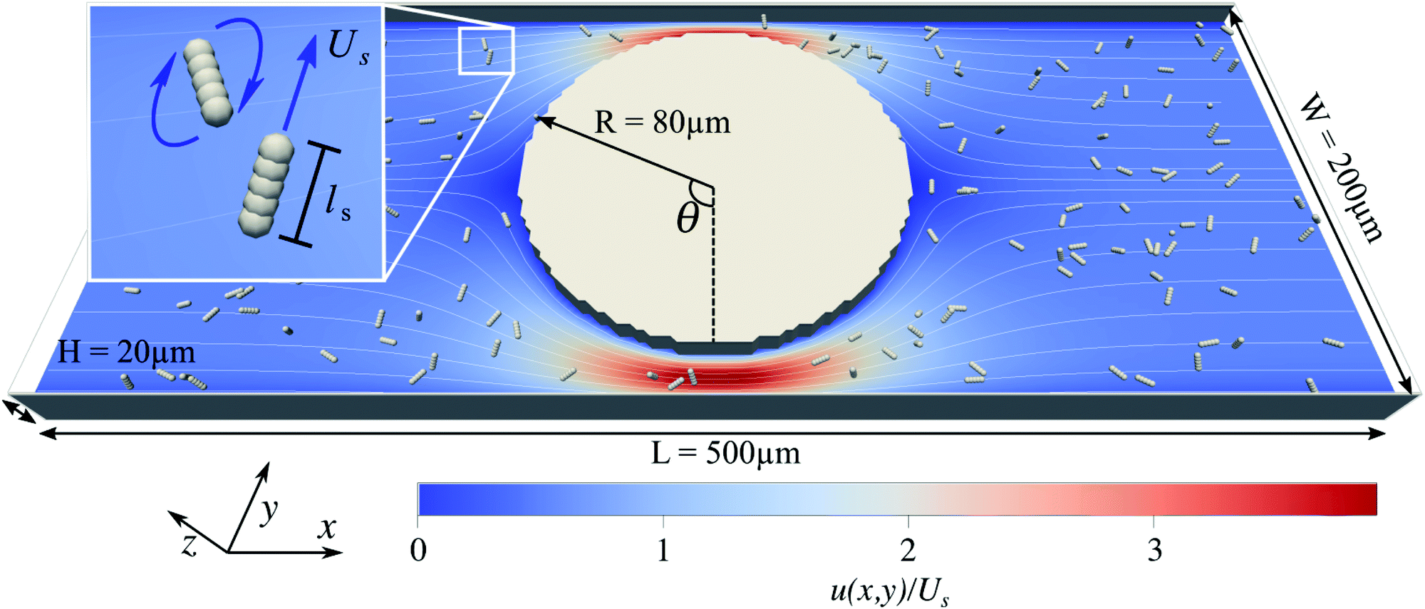

Fig. 1 The simulation set-up consists of a rectangular fluid-filled channel of size (L, W, H) = (500 μm, 200 μm, 20 μm) with a cylindrical obstacle of radius 80 μm placed at the center of the box. Inside the channel are up to 159 swimmers, each consisting of five interaction sites with the lattice-Boltzmann fluid, which are capable of performing run-and-tumble motions as indicated on the inset. The fluid is driven by an external force density. The stream lines and the colormap represent the driven flow-field projected on to the xy-plane normalized by the swimming speed U_s.

We solve the dynamic flow problem by means of the lattice-Boltzmann method^33,34 which can be regarded as a Navier–Stokes solver. The advantages of the algorithm are the simple implementation of complex boundary conditions and the possibility to couple the fluid simulation to the molecular dynamics simulation of the swimmers. Periodic boundary conditions are used along the x-direction, and a no-slip boundary condition is imposed on the top and bottom surfaces (at z = −H/2 and z = H/2), on the lateral walls (at y = −W/2 and y = W/2) of the flow cell, and on the surface of the cylindrical obstacle. The flow is driven through the channel by applying a constant force density onto each lattice-Boltzmann node. To test the correctness of our LB implementation and to investigate the severity of grid artifacts we performed a computational fluid dynamics simulation of the channel using a finite element method. The comparison can be found in the ESI†Fig. 1.⁴²

The system's geometry and the resulting flow field are depicted in Fig. 1. We characterize the flow strength by the average value , i.e., measured at the outlet of the channel. For all performed simulations, the Reynolds number of the flow is very small Re ∼ 10⁻². This is manifested through the spatial symmetries of the flow field with respect to the center of the box. Note that from now on, we always normalize the flow strength by the swimming speed U_s of our model bacteria unless otherwise stated.

B. Swimmer model

In order to reproduce the elongated shape of E. coli the bacteria are modeled as a rigid collection of five aligned molecular dynamics particles (see Fig. 1). A detailed description of the model is given in ref. 41.

A short ranged non-bonded Weeks–Chandler–Anderson interaction potential between the particles making up a swimmer is used to incorporate the swimmer's excluded volume. The body extension is l_s ∼ 5 μm, and the flagella are not modeled explicitly. Thus, the aspect ratio (= body length/diameter) of 5 for the swimmer is within the range of aspect ratios of particles used by Junot et al.²²

All molecular dynamics particles are coupled to the underlying lattice Boltzmann fluid via a point-friction coupling scheme according to ref. 36–39.

The swimmers perform a run-and-tumble motion as observed in some flagellated bacteria like E. coli. The dynamics are characterized by straight swimming phases (runs), interrupted by sudden changes in direction (tumbles).^43–45

Straight swimming motion is, in the present study, obtained by applying a body-fixed force along the main axis of the swimmer. To ensure the force-free swimming mechanism and to mimic the propulsion by flagella rotation, a counter force of equal strength but opposite direction is applied to the fluid behind the swimmer.⁴¹ During the runs, the swimmers can thus be understood as a force-dipole pusher with a constant swimming velocity U_s.^38,39 The numerical parameters (listed in the ESI†⁴²) are chosen such that U_s = 24 μm s⁻¹, which is very close to the average velocity of the bacteria used by Miño et al.⁴⁰

A tumbling motion is initiated by applying two opposite forces at the two terminating molecular dynamics particles of the swimmer, perpendicular to the swimmer's long axis. The two opposite forces create a rotating torque. Again, both forces are balanced by counter-forces on the fluid away from the swimmer to ensure a net-torque-free rotation.

During the simulation, the durations of run and tumble phases, as well as the tumble angles, are randomly drawn from the respective distributions. They reproduce the correct statistics of the run-and-tumble motion such that the (average) run and tumble durations are T_r = 1 s and T_t = 0.1 s, respectively.^43–45 The swimmers’ motion can thus be characterized by the run T_r and tumble T_t durations as well as the swimming speed U_s.

Also note that rotation or translation of a swimmer through thermal noise is not considered in our study since the effects of thermal diffusion are several orders of magnitude lower than those of the run-and-tumble motion.

We introduce N = 159 swimmers to the system to achieve the low density of bacteria used in ref. 40. In the following we analyze the swimmer distribution in the channel in various situations. We hence define the swimmer distribution ρ(r) as

where r_i(t) is the ith swimmer's position at time t, and T the total simulation length. It is a time-averaged one-particle distribution. The projection onto the xy-plane is then done by taking the average over the z-direction: . We make the swimmer distribution ρ(r) dimensionless by normalizing it with the homogeneous swimmer density ρ_h = N/V_box, where V_box is the volume of the simulation box that is accessible to swimmers, i.e., excluding the volume occupied by the obstacle.

Here, we define some quantities that are useful in describing our observation. The swimmer distribution around the obstacle ρ_obs(θ) as a function of polar angle θ is given by 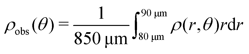. Similarly, the swimmer distribution on the lateral walls ρ_wall(x) at y = −W/2 and y = W/2 as a function of lateral position x is 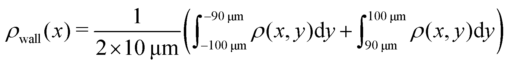. Consequently, we calculate the swimmer density behind the obstacle using 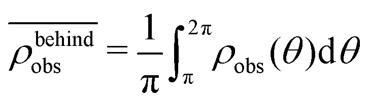and on the lateral walls using .

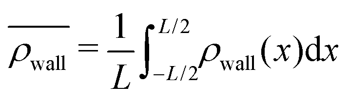III. Results

A. Accumulation is caused by niches

Fig. 2 shows the spatial distribution of swimmers calculated using eqn (1) inside the system box for different flow conditions. Additionally, Fig. 3(a) and 4 quantitatively present the spatial distribution of the swimmers around the obstacle and on the lateral walls, respectively. Notice first that, in the absence of flow, a significantly large fraction of swimmers (i.e., ρ > ρ_h) is distributed both on the lateral walls and around the obstacle. The bulges of the blue curve in Fig. 3(a) at θ = 0° and 180°, as well as that of the blue curve in Fig. 4 at x = 0 show a small enhancement of the accumulation at places where the obstacle and the lateral walls are closest. We refer to these regions as constrictions. The homogeneous swimmer accumulation on the surfaces, i.e., both on the lateral walls and on the obstacle, is to be expected,^46–49 since at the chosen running duration, the persistent swimming length scale (l_per = 24 μm) is comparable to the length scales in the channel; because the swimmers swim in all possible directions with equal probability, at some point they will touch a surface and stay there until tumble events orient their swimming directions away from the surface.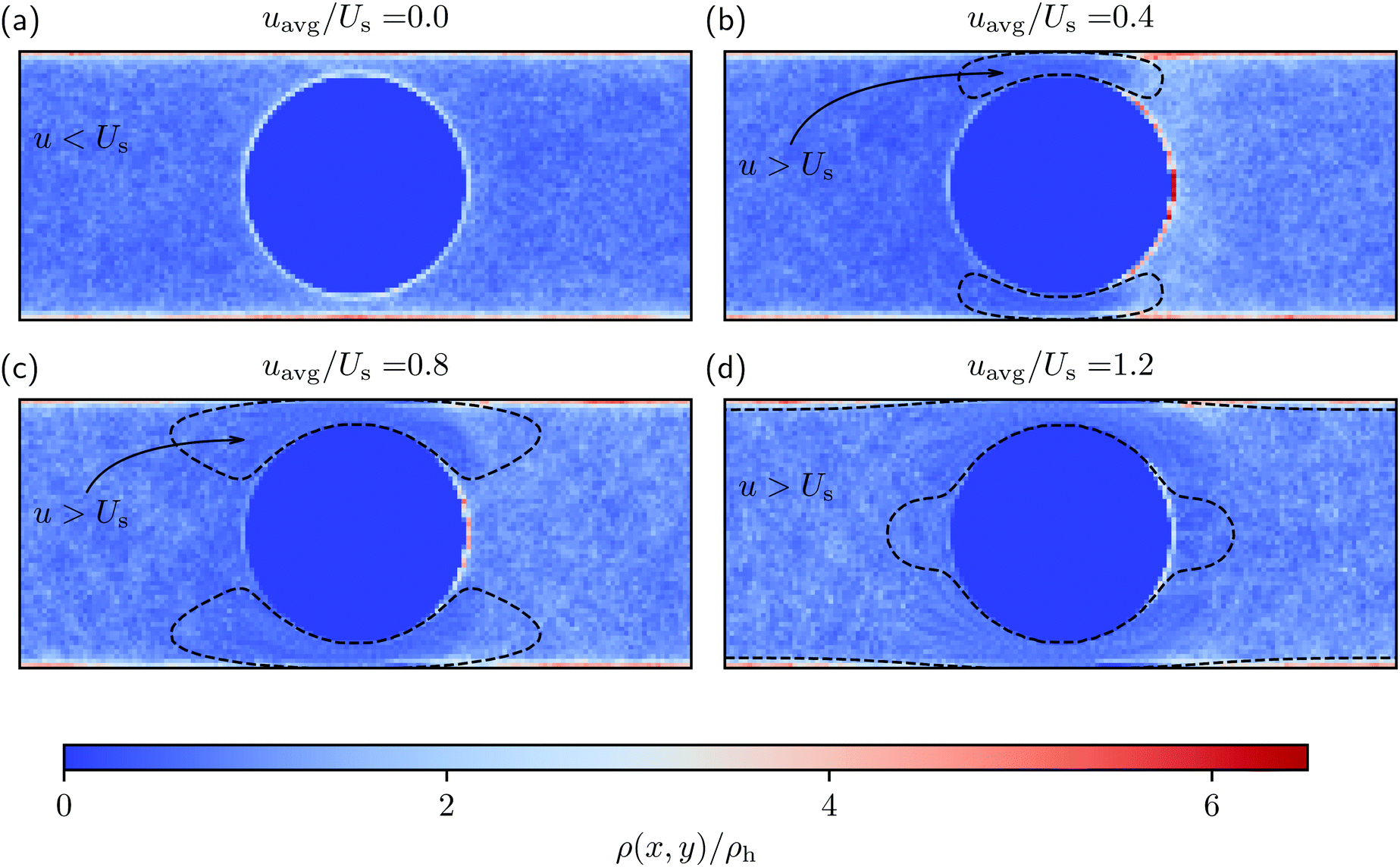

Fig. 2 The swimmer distribution ρ(x,y) normalized with the homogeneous swimmer distribution ρ_h in the channel for various external flow inputs. The dashed lines are contours, separating the regions where the magnitude of flow velocity u(x,y), averaged in the z-direction, is greater than the magnitude of the swimming velocity U_s.

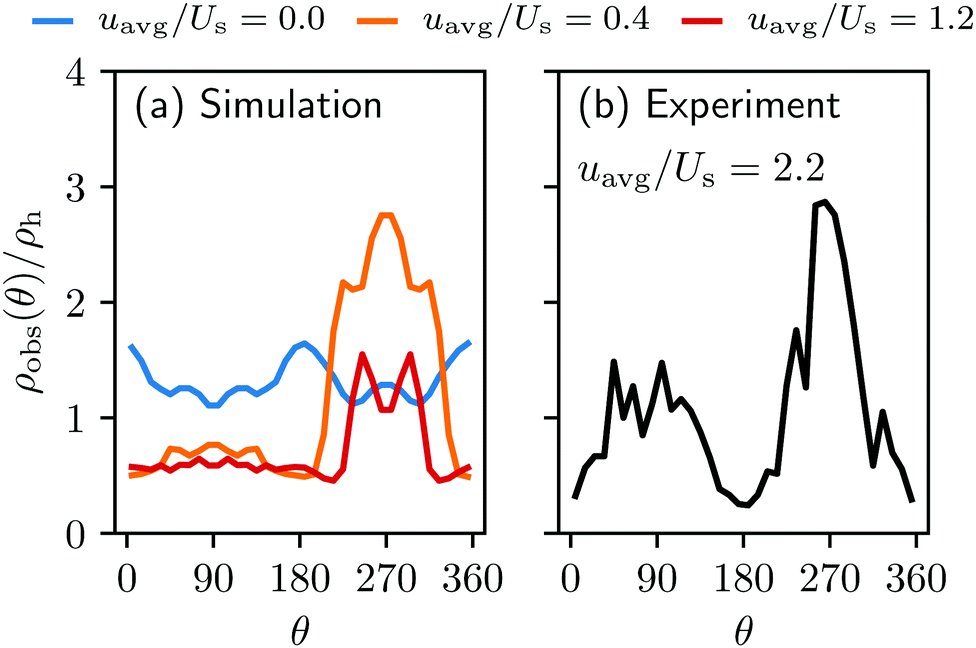Fig. 3 The normalized swimmer distribution around the obstacle ρ_obs/ρ_h in (a) the simulation and (b) the experiment (ref. 40) as a function of the polar angle around the center of the obstacle. θ = 0 and 180 correspond to the lateral sides, and θ = 90° and θ = 270° to the upstream and downstream sides, respectively. The blue, orange and red lines in (a) stand for the velocity ratios u_avg/U_s = 0.0, 0.4, and 1.2.

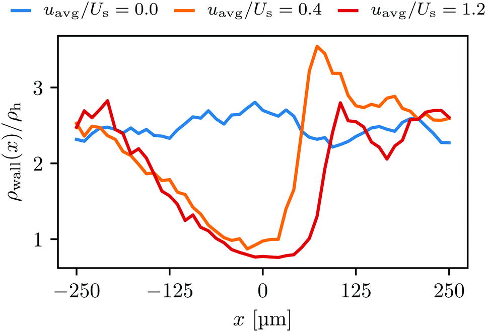Fig. 4 The normalized swimmer distribution along the lateral walls ρ_w/ρ_h for different flow velocities. The blue, orange and red lines stand for u_avg/U_s = 0.0, 0.4, and 1.2, respectively.

Additionally, we observe that more swimmers are accumulated on the lateral walls than around the obstacle. This can be explained by the geometric characteristics of the surfaces. The obstacle is a convex surface, and not capable of containing swimmers for as long as the flat walls can do.^27,28 We attribute this to the simple fact that the swimmers will depart from any convex surface merely by swimming straight in any direction that was initially tangent to the surface. The influence of the convexity will become more significant with increasing running duration T_r.

Introducing an external flow, we measure an inhomogeneous distribution of swimmers on the surfaces. A larger number of swimmers accumulates on the downstream side of the obstacle while the density of swimmers on the upstream side of the obstacle is reduced, falling below the homogeneous swimmer density ρ_h. For u_avg/U_s = 0.2 nearly three times more swimmers per unit of volume are located at the rear of the obstacle than anywhere else in the fluid. This finding is in agreement with the observation made in the experiment Miño et al.⁴⁰

We furthermore find that stronger flow velocities reduce the extension of the regions where the accumulation is observed. Consequently, the swimmer densities behind the obstacle and on the lateral walls reduce with increasing external flow strength, as indicated by the solid lines in Fig. 5. To explain this, we mark the regions where the magnitude of the local flow velocity is higher than the swimming velocity U_s in Fig. 2. For u_avg/U_s < 1.0, the regions where u > U_s are localized in the constrictions. At the strongest external flow (u_avg/U_s = 1.2), the region covers the entire channel apart from two small domains located at the rear and front of the obstacle, and parts of the lateral walls located away from the constrictions.

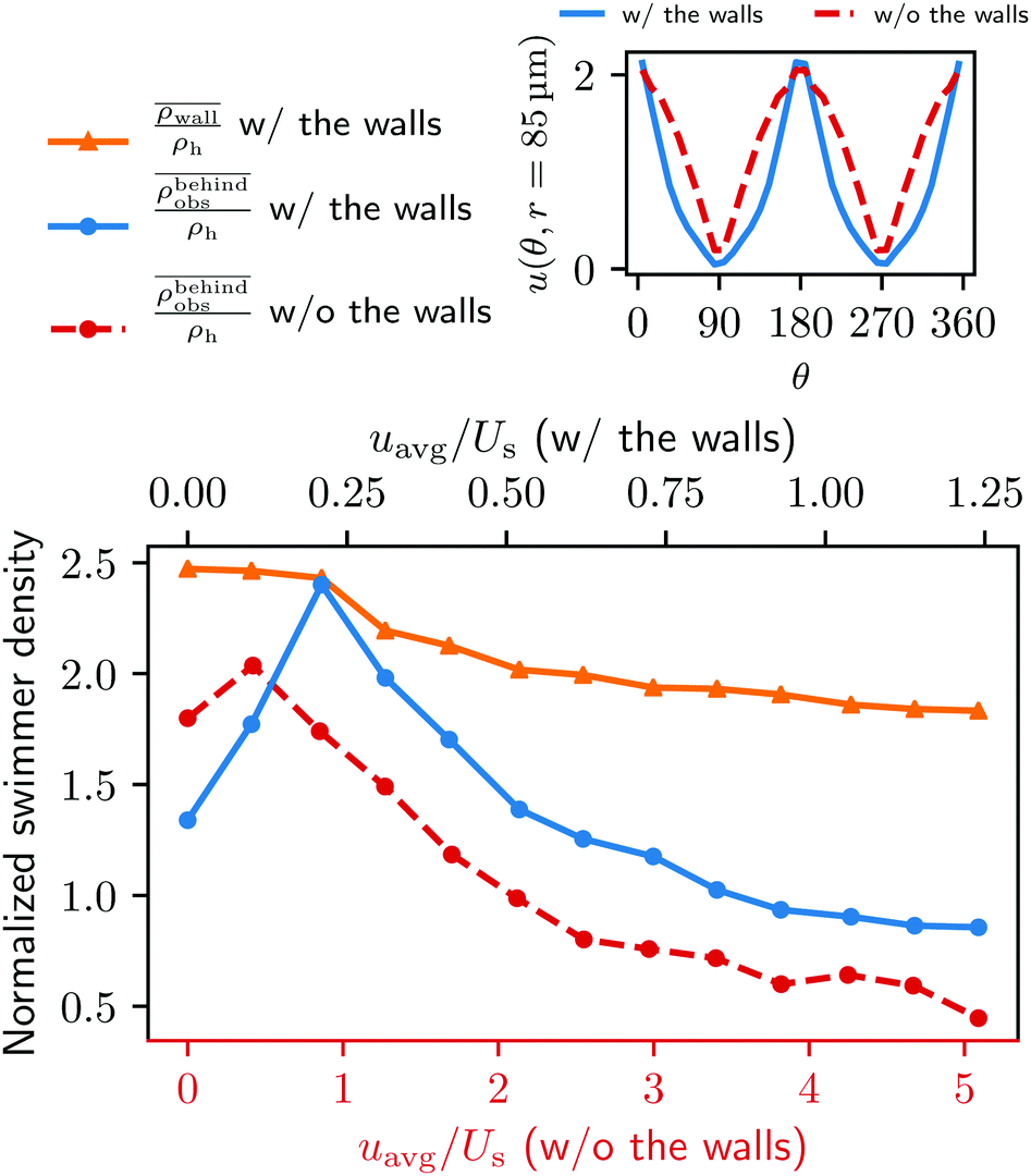Fig. 5 Main: The average swimmer density behind the obstacle (blue solid line), and on the walls (orange solid line) as a function of the external flow strength u_avg/U_s in the presence of the lateral walls, as well as the average swimmer density behind the obstacle in the absence of the lateral walls (red dashed line). Top inset: the flow velocity u(θ,r = 34σ)/u_avg around the obstacle as a function of polar angle θ for both cases, with (blue), and without (red) the lateral walls.

Higher local flow speed regions act as one way streets; all swimmers are moving down-stream regardless of their swimming direction, since they cannot compete with the flow. The borders of the stronger flow regions therefore act as a “niches” in which the upstream swimmers stay until they reorient. This effect leads to an asymmetric distribution of swimmers, with a higher density in the right half of the channel.

The niche argument implies that many swimmers that accumulate behind the obstacle are swimming against the local flow direction. To support this argument we calculate, as shown in Fig. 6, the ratio of the number of events where a swimmer enters the accumulation region by swimming upstream to the total number of entering events. This ratio stays roughly constant at a high value of about 70% irrespective of the increasing external flow. This is in contrast to the ratio of upstream swimming bacteria in the whole system (N_up/N), which decreases monotonically with increasing external flow. From the two curves we can conclude that the smaller number of accumulated swimmers behind the obstacle is due to the fact that the total number of swimmers that are capable of accumulating is reduced. The mechanism of accumulation itself (upstream swimming into niches) remains unaltered despite the increasing external flow.

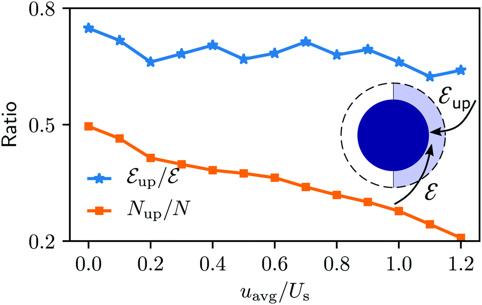Fig. 6 Blue solid line: The ratio of the number of events where upstream swimmers enter behind the obstacle to that of events where swimmers enter behind the obstacle regardless of their swimming directions. Red: The time averaged ratio of the number N_up of swimmers that swim upstream in the whole system to the total number N of swimmers. A swimmer is counted as upstreaming if the x-component of its velocity in the laboratory frame is non-positive. Inset: A schematic visualization of events and .

The accumulation behind the obstacle (blue curve in Fig. 5) displays a non-monotonic behavior which can be explained as follows. With a very weak external flow, the available space for the swimmers to accumulate is relatively large. The number of swimmers reaching the rear is thus reduced, because a large fraction is accumulated elsewhere. The accumulation exhibits a maximum around u_avg/U_s = 0.2. This value coincides with the flow strength at which the local flow speed at the constriction becomes larger than the bacterial swimming speed. The one way street mechanism now leads to the maximum accumulation because the constrictions effectively block the upstream swimmers but the overall flow speed is not yet strong enough to flush the swimmers. With a further increase of the external flow strength, the size of the niche shrinks, as can be observed in Fig. 2. Naturally, this limits the accessible surface area, and therefore the accumulation decreases.

B. Role of lateral walls on accumulation

In this part we will analyze in detail the effects that the lateral walls play in the bacterial accumulation. Looking back again into Fig. 2, we also note the preferential accumulation of the bacteria in the right half of the channel. This means that the niche argument also applies to the accumulation on the lateral walls. Moreover, a significant number of bacteria accumulate on the walls regardless of external flow strength. We argue that these accumulated swimmers on the walls can potentially migrate to the obstacle.

Due to the geometry, the lateral walls orient the swimmers to the ±x directions as they slide along. The upstreaming fraction can travel along the channel even under strong external flow, as the no-slip boundary condition provides niches of low flow velocities. Using this route, a swimmer can move up to the constriction with a high probability. Behind the constriction, the streamlines fan out and depart from the wall. This flow away from the walls causes the bacteria to reorient and turn towards to the cylinder, as can be seen in Video S1, ESI.† ⁴²

The swimmers’ transitions from one surface to another can be easily calculated from the trajectories, and the results are displayed in Fig. 7. In Fig. 7 one can see that the from-wall-to-obstacle transition K_w,o happens more often than the from-obstacle-to-obstacle transition K_o,o across the board. Thus, without lateral walls, one may expect a smaller accumulation around the obstacle.

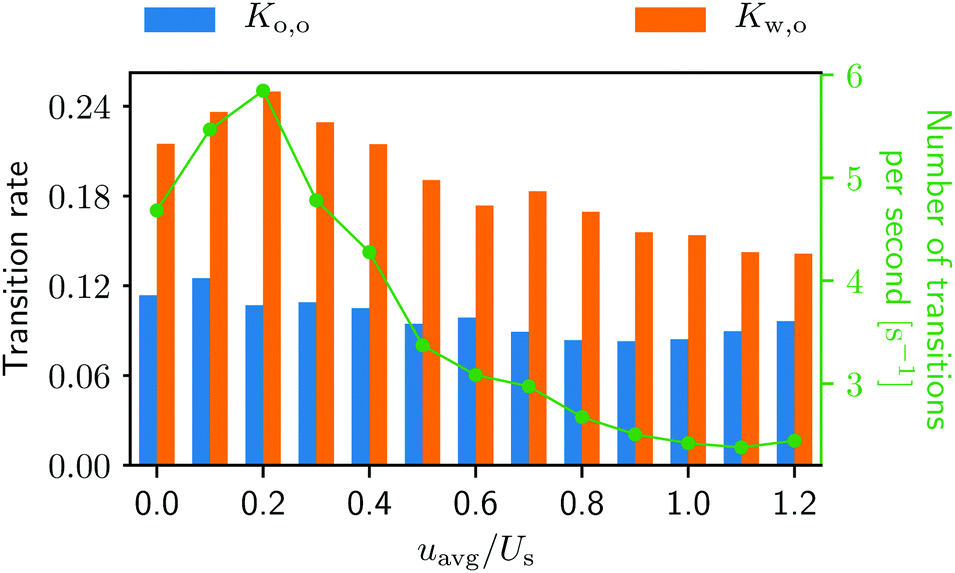Fig. 7 Transition rates K_o,o for the from-obstacle-to-obstacle and K_w,o for the from-wall-to-obstacle as a function of external flow strength. The green curve represents the combined number of transitions per second. More detailed information can be found in Fig. 2, ESI.† ⁴²

To quantify our argument above, we also performed a new set of simulations in which the lateral walls were removed and replaced by a periodic boundary condition in the y direction. To make the new system as comparable to the one with the walls, the system size is also changed to (L, W, H) = (500 μm, 500 μm, 20 μm). In addition, we adjusted the force densities, such that the flow velocity and profile around the obstacle are as close as possible to the original geometry (see the top right inset in Fig. 5). The total number of swimmers is changed from 159 to 248 to obtain better statistics. Notice that the change in the total number of swimmers does not affect the overall dynamics of the total system since we remain in the low density limit.

In the absence of lateral walls, only a relatively small accumulation behind the obstacle is found, except for the first two smallest external flow conditions as represented by the red dashed line in Fig. 5. This is because with a very weak external flow strength, the swimmers can accumulate on any surface. Without the lateral walls, it is thus natural that more swimmers accumulate at the cylinder. With a stronger external flow strength, however, the swimmers without a lateral confinement will only end up behind the obstacle if a tumble happens at the right time with the right angle to allow them to come close to the surface of the obstacle. Therefore, for most of the time, the bacteria are just following the fluid flow.

Notice also that in Fig. 7 the green curve, i.e., the total number of transitions per second, as well as the from-wall-to-obstacle transition K_w,o as a function of the external flow strength resemble that of the normalized swimmer density in Fig. 5. To explain this we resort to Fig. 4. If the external flow strength is very weak, the swimmers on the walls are distributed rather homogeneously, meaning that many of the swimmers are located far away from the obstacle. The migration from the walls to the obstacle, consequently, happens less frequently. As the external flow gets stronger, however, the swimmers preferably accumulate on the wall at x ∼ 120 μm, which is close to the obstacle. Now the swimmers have to overcome only a shorter distance to arrive at the obstacle, which enhances the from-wall-to-obstacle transition K_w,o.

C. Influence of swimming characteristics

In order to understand the physics behind the bacterial accumulation mechanisms better, we also investigate the influence of the running duration T_r. We keep the external flow strength fixed at u_avg = 0.6U_s.

In Fig. 8 we display the swimmer densities behind the obstacle and on the lateral walls as a function of T_r ∈ [0.16 s, 21 s]. Intriguingly, the swimmer accumulation behind the obstacle peaks, and then decreases, whereas the bacterial density on the walls monotonically increases.

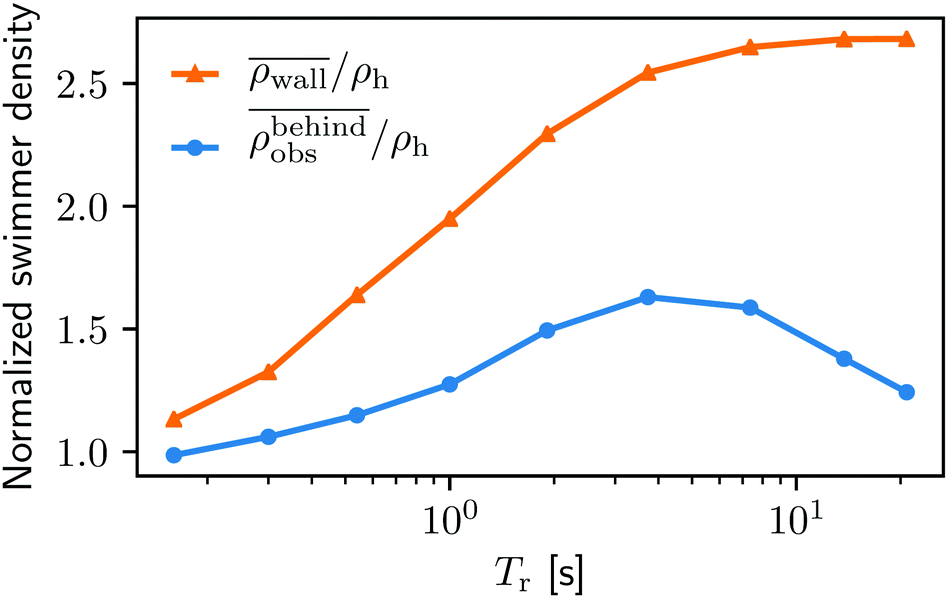Fig. 8 The normalized swimmer density behind the obstacle (blue solid line) and on the lateral walls (orange solid line) as a function of the (average) running duration T_r.

When T_r is very small, the behavior of the swimmers is similar to Brownian motion of passive particles. As they change their direction rapidly, their swimming only leads to enhanced diffusion, but not to persistent motion. For a visualization of this effect we refer to Video S2, ESI.† ⁴² The lack of persistent motion yields a very small accumulation density on the boundaries.

As T_r increases, the swimmers start showing an increasing persistent and directed motility that allows them to swim for a sufficient amount of time to reach the boundaries.

With a very large T_r(>7 s), however, the situations on the walls and behind the obstacle start diverging. This is primarily due to the shape of the boundaries as mentioned in Section IIIA. The swimmers with very high T_r rarely change their directions. Therefore, the walls can trap swimmers much longer than the obstacle. Note that similar observations are reported by Spagnolie et al.²⁷ and Sipos et al.²⁸ Although without flow, the studies identify an optimal obstacle size for a hydrodynamic capture, and point out, as in the present study, the key role of a surface geometry on the accumulation of microswimmers.

The running duration plays a substantial role in the transition behavior as well (see Fig. 9). As T_r gets larger, the migration from the walls to the obstacle happens more often. On the other hand, the from-obstacle-to-obstacle transition happens less frequent with increasing T_r. One shall keep in mind, however, that this transition at a very small T_r is a rather trivial transition. At very small T_r a swimmer is essentially a passive Brownian particle, jiggering back and forth to the obstacle, making a number of meaningless “transitions”. Such transitions, however, become less probable as T_r increases (also see Videos S1 and S3, ESI†⁴² and compare the swimmers' behaviors).

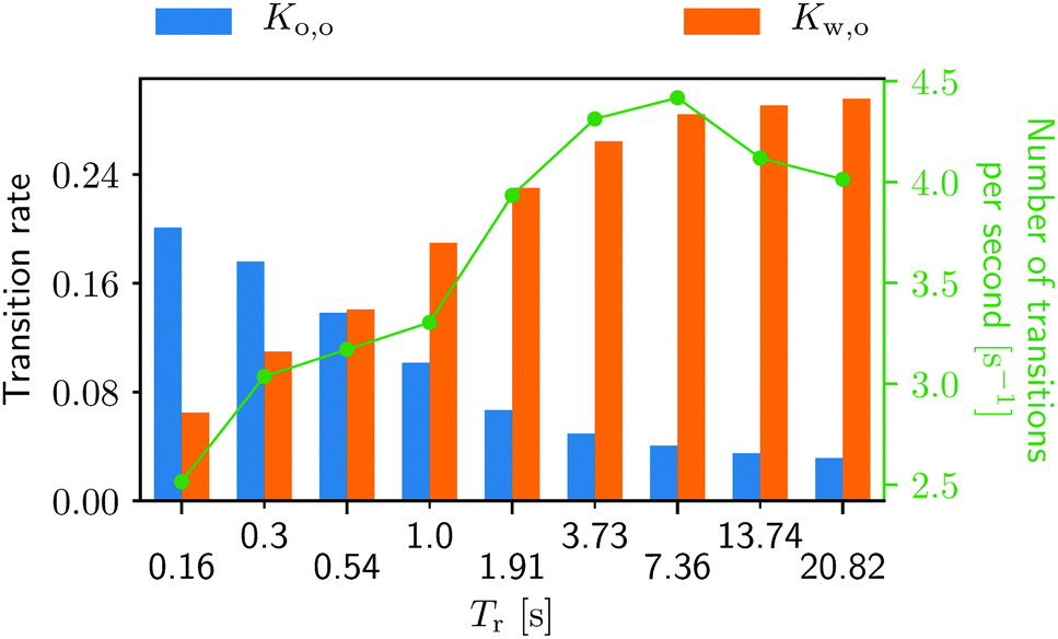Fig. 9 Transition rates for the from-obstacle-to-obstacle K_o,o and for the from-wall-to-obstacle rate K_w,o as a function of the (average) running duration T_r. The green curve represents the combined number of transitions per second. More detailed information can be found in Fig. 3, ESI.† ⁴²

The number of transitions per second in Fig. 9 also increase with growing T_r until T_r = 7.36 s, and then start decreasing. Fixed by the system's geometry, we can find the optimal running duration for the accumulation behind the obstacle around T_r ∼ 4 from Fig. 8 and 9. It is worth noting that the swimming Péclet number, the ratio of the persistent running length (= U_sT_r) to the body size, is not a control parameter when it comes to the bacterial accumulation in porous media. This is because the ratio of local fluid flow speed to the swimming speed also affects the accumulation as discussed above.

D. Limitations of the coarse-grained bacterial model

Our bacterial model and the simulation could reproduce qualitatively the preferred accumulation behind the obstacle as observed in the experiment of Mino et al.,⁴⁰ but there remains a quantitative discrepancy. The simulations overall yielded a smaller accumulation density around the obstacle than found in the experiment. In the simulation, the swimmers were mostly washed away when the average flow speed exceeded u_avg = 1.2U_s, whereas in the experiment, the bacteria could manage to accumulate even under a stronger external flow of u_avg ∼ 2.2U_s. The difference in accumulation density was found particularly pronounced in front of the obstacle.

Despite the fact that one should not over-interpret results obtained by coarse-grained models, we present three reasons for this discrepancy. First, the swimming speed of our bacterial model was kept constant in the simulation in order to achieve a better understanding of the interplay between the local flow field and the swimmers’ motility. In the experiment, the bacterial swimming speed distribution follows a half-normal distribution with a standard deviation that is roughly of size U_s.⁴⁰ This means that numerous bacteria are able to swim faster than U_s and therefore more of them can accumulate behind the obstacle. In addition to this, the discrepancy may also be due to the fact that we did not introduce any attractive interaction between the swimmers and the boundaries. It is well known that E. coli can adhere to surfaces via a short range electrostatic interaction,^50,51 and they also can interact with the obstacle via pili. Finally, we neglected the rotation of the bacterial body around its main axis and the counter-rotation of the flagella that causes the bacteria to swim in circular trajectories on surfaces.¹⁹ This will result in a lower effective diffusivity, and can cause the bacteria to explore less space in a given time compared to straight swimming. In front of the obstacle, bacteria will escape the region of small flow by swimming in any direction (except straight into the cylinder), so only circular swimming could cause the prolonged residence time in this area.

IV. Conclusions

Our simulations demonstrated that motile microorganisms preferably accumulate in regions where the fluid speed is lower than the swimming speed, which are referred to as niches. For the geometry considered here, the niches are located behind the obstacle (in direction of the external force density) and on the lateral surfaces. Especially, when it comes to the accumulation behind the obstacle, we showed that upstream swimming of swimmers plays an important role. This conclusion is in line with the recent results reported by Alonso-Matilla et al.¹⁰ and Secchi et al.²⁶ In the first study, they investigated the dispersion of swimmers in a matrix of an obstacle, whose shape is systematically altered from a circle to an ellipsoid and to a triangle. They showed that, as long as an external flow is moderate, such an upstream swimming pattern can be observed not only with circular obstacles but also with triangular obstacles, the edges of which are pointing to the downstream direction. This suggests that the niche argument is not restricted to a cylindrical obstacle. In the second study, they used a microfluidic chip containing circular pillars of different diameters, and observed more bacteria at the downstream side of the obstacles. They identified the shear induced reorientation as the mechanism allowing the bacteria to accumulate in these specific regions. Using a similar approach, Słomka et al.⁵² came to the conclusion that the reorientation is also responsible for the accumulation of motile bacteria at the rear of a sinking spherical particle. In both studies, the shear induced by the flow around the obstacles is the physical mechanism, explaining the accumulation of the bacteria. In the present study, the confinement by lateral walls also plays a substantial role on the swimmer accumulation behind the obstacle. These walls produce additional zones of small fluid velocity due to the no-slip boundary condition which provide a pathway for the bacteria to swim upstream. This mechanism is an important element since it allows swimmers to come closer to the constrictions, from which the swimmers can migrate to the obstacle. The accumulation of bacteria by the surface is triggered by the local shear that reorients the bacteria toward the surface. We note that a model where bacteria are replaced by rod like particles^23,26 that are reoriented by the shear is sufficient to capture this process. However, because the hydrodynamic and the steric interactions between the surface and the bacteria are the key mechanisms leading to the “trapping” of the bacteria by the surface,⁵³ rod-like approaches fail to model the swimming along the surface. Our model includes the hydrodynamic and steric effects, and thus is successful in taking into account the effect of the lateral surfaces on the accumulation. Finally, we observe that an optimal bacterial accumulation can be achieved when the running duration is around 7 s. These observations can help to design and optimize strategies to sort and trap microorganisms. It also can reveal insights into the physical mechanisms important for the filtration of motile bacteria in porous media.

Our study shows that the bacterial model coupled to a LB fluid is an efficient technique to simulate motile microorganisms at the pore scale including hydrodynamic and steric interactions. The LB method enables us, in principle, to consider arbitrary complex 3D pore geometries and flow conditions⁵⁴ easily. For these reasons, we believe that our approach can be used in future work to study the influence of flow on the “hopping and trapping” complex dynamics of bacteria recently observed in confined environment.^12,13 A strong advantage of the model is the ability to simulate many interacting micro swimmers, opening up the possibility to study collective effects in denser solutions. The bacterial swimming characteristics can be easily adapted to reproduce other types of bacteria. In the present article, the swimmers are of the pusher type, like E. coli, but the method can be implemented to consider neutral swimmers or pullers as well. Some algae, for example, fall into the last category. Another advantage of our model is that the persistence swimming time and the tumbling dynamics can also be modified to incorporate more complex stochastic dynamics. In total our model could be easily extended to investigate other important systems from the point of view of applications.

Conflicts of interest

There are no conflicts to declare.

Acknowledgements

M. L, C. L., K. S. and C. H. were funded by the Deutsche Forschungsgemeinschaft (DFG, German Research Foundation) – Project Number 327154368 – SFB 1313, and the SPP 1726 “Microswimmers: from single particle motion to collective behavior”, grant HO1108/24-2. H. A. is supported by public grants overseen by the French National Research Agency (ANR): (i) ANR Bacflow AAPG 2015 and (ii) from the “Laboratoire dExcellence Physics Atom Light Mater” (LabEx PALM) as part of the “Investissements dAvenir” program (reference: ANR-10-LABX-0039-PALM).

References

1. G. Pandey and R. K. Jain, Bacterial chemotaxis toward environmental pollutants: Role in bioremediation, Appl. Environ. Microbiol., 2002, 68, 5789–5795,  DOI:10.1128/AEM.68.12.5789-5795.2002.
2. C. M. Aitken, D. M. Jones and S. R. Larter, Anaerobic hydrocarbon biodegradation in deep subsurface oil reservoirs, Nature, 2004, 43, 291–294.
3. ed. E. C. Donaldson, G. V. Chilingarian and T. F. Yen, Developments in Petroleum Science, Elsevier, 1989, vol. 22,  DOI:10.1016/S0376-7361(09)70084-6. http://www.sciencedirect.com/science/article/pii/S0376736109700846.
4. I. Lazar, I. G. Petrisor and T. F. Yen, Microbial enhanced oil recovery (meor), Pet. Sci. Technol., 2007, 250(11), 1353–1366,  DOI:10.1080/10916460701287714.
5. L. R. Brown, Microbial enhanced oil recovery (meor), Curr. Opin. Microbiol., 2010, 130(3), 316–320,  DOI:10.1016/j.mib.2010.01.011 , http://www.sciencedirect.com/science/article/pii/S1369527410000160.
6. A. Dadda, C. Geindreau, F. Emeriault, S. Rolland du Roscoat, A. Garandet, L. Sapin and A. Esnault Filet, Characterization of microstructural and physical properties changes in biocemented sand using 3d X-ray microtomography, Acta Geotech, 2017, 12, 955–970,  DOI:10.1007/s11440-017-0578-5.
7. T. Marzin, B. Desvages, A. Creppy, A. E.-F. Louis Lépine and H. Auradou, Using microfluidic set-up to determine the adsorption rate of sporosarcina pasteurii bacteria on sandstone, Transp Porous Med, 2020, 132, 283–297,  DOI:10.1007/s11242-020-01391-3.
8. W. De Muynck, N. De Belie and W. Verstraete, Microbial carbonate precipitation in construction materials: A review, Ecol. Eng., 2010, 360(2), 118–136,  DOI:10.1016/j.ecoleng.2009.02.006 , http://www.sciencedirect.com/science/article/pii/S092585740900113X. Special Issue: BioGeoCivil Engineering.
9. N. Pal Kaur, S. Majhi, N. Kaur Dhami and A. Mukherjee, Healing fine cracks in concrete with bacterial cement for an advanced non-destructive monitoring, Constr. Build. Mater., 2020, 242, 118151,  DOI:10.1016/j.conbuildmat.2020.118151.
10. R. Alonso-Matilla, B. Chakrabarti and D. Saintillan, Transport and dispersion of active particles in periodic porous media, Phys. Rev. Fluids, 2019, 40(4), 043101,  DOI:10.1103/PhysRevFluids.4.043101.
11. X. Yang, R. Parashar, N. L. Sund, A. E. Plymale, T. D. Scheibe, D. Hu and R. T. Kelly, On modeling ensemble transport of metal reducing motile bacteria, Sci. Rep., 2019, 9, 14638,  DOI:10.1038/s41598-019-51271-0.
12. T. Bhattacharjee and S. S. Datta, Bacterial hopping and trapping in porous media, Nat. Commun., 2019, 100(1), 1–9.
13. T. Bhattacharjee and S. S. Datta, Confinement and activity regulate bacterial motion in porous media, Soft Matter, 2019, 150(48), 9920–9930.
14. D. Scheidweiler, F. Miele, H. Peter, T. J. Battin and P. de Anna, Trait-specific dispersal of bacteria in heterogeneous porous environments: from pore to porous medium scale, J. R. Soc., Interface, 2020, 170(164), 20200046,  DOI:10.1098/rsif.2020.0046 , https://royalsocietypublishing.org/doi/abs/10.1098/rsif.2020.0046.
15. P. de Anna, A. A. Pahlavan, Y. Yawata, R. Stocker and R. Juanes, Chemotaxis under flow disorder shapes microbial dispersion in porous media, Nat. Phys., 2020 DOI:10.1038/s41567-020-1002-x.
16. T. Kaya and H. Koser, Direct upstream motility in escherichia coli, Biophys. J., 2012, 1020(7), 1514–1523,  DOI:10.1016/j.bpj.2012.03.001.
17. V. Kantsler, J. Dunkel, M. Blayney and R. E. Goldstein, Rheotaxis facilitates upstream navigation of mammalian sperm cells, eLife, 2014, 3, e02403,  DOI:10.7554/eLife.02403.
18. N. Figueroa-Morales, G. Leonardo Miño, A. Rivera, R. Caballero, E. Clément, E. Altshuler and A. Lindner, Living on the edge: transfer and traffic of e. coli in a confined flow, Soft Matter, 2015, 11, 6284–6293,  10.1039/C5SM00939A.
19. E. Lauga, W. R. DiLuzio, G. M. Whitesides and H. A. Stone, Swimming in circles: Motion of bacteria near solid boundaries, Biophys. J., 2006, 900(2), 400–412 , http://www.sciencedirect.com/science/article/pii/S0006349506722214.
20. A. J. T. M. Mathijssen, N. Figueroa-Morales, G. Junot, É. Clément, A. Lindner and A. Zöttl, Oscillatory surface rheotaxis of swimming e. coli bacteria, Nat. Commun., 2019, 100(1), 1–12.
21. R. Rusconi and R. Stocker, Microbes in flow, Curr. Opin. Microbiol., 2015, 25, 1–8,  DOI:10.1016/j.mib.2015.03.003.
22. G. Junot, N. Figueroa-Morales, T. Darnige, A. Lindner, R. Soto, H. Auradou and E. Clément, Swimming bacteria in poiseuille flow: The quest for active bretherton-jeffery trajectories, EPL, 2019, 1260(4), 44003,  DOI:10.1209/0295-5075/126/44003.
23. R. Rusconi, J. S. Guasto and R. Stocker, Bacterial transport suppressed by fluid shear, Nat. Phys., 2014, 100(3), 212–217.
24. A. Creppy, E. Clément, C. Douarche, M. V. D’Angelo and H. Auradou, Effect of motility on the transport of bacteria populations through a porous medium, Phys. Rev. Fluids, 2019, 4, 013102,  DOI:10.1103/PhysRevFluids.4.013102.
25. A. Dehkharghani, N. Waisbord, J. Dunkel and J. S. Guasto, Bacterial scattering in microfluidic crystal flows reveals giant active taylor-aris dispersion, Proc. Natl. Acad. Sci. U. S. A., 2019, 1160(23), 11119–11124,  DOI:10.1073/pnas.1819613116.
26. E. Secchi, A. Vitale, G. L. Miño, V. Kantsler, L. Eberl, R. Rusconi and R. Stocker, The effect of flow on swimming bacteria controls the initial colonization of curved surfaces, Nat. Commun., 2020, 110(1), 1–12.
27. S. E. Spagnolie, G. R. Moreno-Flores, D. Bartolo and E. Lauga, Geometric capture and escape of a microswimmer colliding with an obstacle, Soft Matter, 2015, 110(17), 3396–3411,  10.1039/c4sm02785j.
28. O. Sipos, K. Nagy, R. Di Leonardo and P. Galajda, Hydrodynamic trapping of swimming bacteria by convex walls, Phys. Rev. Lett., 2015, 114, 258104,  DOI:10.1103/PhysRevLett.114.258104.
29. K. Drescher, Y. Shen, B. L. Bassler and H. A. Stone, Biofilm streamers cause rapid clogging, Proc. Natl. Acad. Sci. U. S. A., 2013, 1100(11), 4345–4350,  DOI:10.1073/pnas.1300321110.
30. K. Z. Coyte, H. Tabuteau, E. A. Gaffney, K. R. Foster and W. M. Durham, Microbial competition in porous environments can select against rapid biofilm growth, Proc. Natl. Acad. Sci. U. S. A., 2017, 1140(2), E161–E170.
31. B. Ezhilan and D. Saintillan, Transport of a dilute active suspension in pressure-driven channel flow, J. Fluid Mech., 2015, 777, 482–522,  DOI:10.1017/jfm.2015.372.
32. B. Ezhilan, R. Alonso-Matilla and D. Saintillan, On the distribution and swim pressure of run-and-tumble particles in confinement, J. Fluid Mech., 2015, 781, R4,  DOI:10.1017/jfm.2015.520.
33. S. Succi, The lattice Boltzmann equation for fluid dynamics and beyond, Oxford University Press, New York, USA, 2001.
34. T. Krüger, H. Kusumaatmaja, A. Kuzmin, O. Shardt, G. Silva and E. M. Viggen, The Lattice Boltzmann Method: Principles and Practice, Springer, Cham, 2017.  DOI:10.1007/978-3-319-44649-3.
35. B. Dünweg and A. J. C. Ladd. Lattice Boltzmann simulations of soft matter systems. in Advanced Computer Simulation Approaches for Soft Matter Sciences III, volume 221 of Advances in Polymer Science, Springer-Verlag Berlin, Berlin, Germany, 2009, pp. 89–166 DOI:10.1007/12_2008_4.
36. B. Dünweg, U. D. Schiller and A. J. C. Ladd, Progress in the understanding of the fluctuating lattice Boltzmann equation, Comput. Phys. Commun., 2009, 1800(4), 605–608.
37. P. Ahlrichs and B. Dünweg, Simulation of a single polymer chain in solution by combining lattice Boltzmann and molecular dynamics, J. Chem. Phys., 1999, 1110(17), 8225–8239.
38. J. de Graaf, H. Menke, A. J. T. M. Mathijssen, M. Fabritius, C. Holm and T. N. Shendruk, Lattice-Boltzmann hydrodynamics of anisotropic active matter, J. Chem. Phys., 2016, 1440(13), 134106,  DOI:10.1063/1.4944962.
39. J. de Graaf, A. J. T. M. Mathijssen, M. Fabritius, H. Menke, C. Holm and T. N. Shendruk, Understanding the onset of oscillatory swimming in microchannels, Soft Matter, 2016, 120(21), 4704–4708,  10.1039/C6SM00939E.
40. G. L. Miño, M. Baabour, R. Chertcoff, G. Gutkind, E. Clément, H. Auradou and I. Ippolito, E coli accumulation behind an obstacle, Adv. Microbiol., 2018, 8, 451–464,  DOI:10.4236/aim.2018.86030.
41. M. Lee, K. Szuttor and C. Holm, A computational model for bacterial run-and-tumble motion, J. Chem. Phys., 2019, 150, 174111,  DOI:10.1063/1.5085836.
42. Note 1. ESI†.
43. H. C. Berg and D. A. Brown, Chemotaxis in escherichia coli analysed by three-dimensional tracking, Nature, 1972, 239(0), 500–504,  DOI:10.1038/239500a0.
44. H. C. Berg. Random Walks in Biology. Princeton University Press, 1993.
45. J. Saragosti, P. Silberzan and A. Buguin, Modeling e. coli tumbles by rotational diffusion. implications for chemotaxis, PLoS One, 2012, 70(4), e35412,  DOI:10.1371/journal.pone.0035412.
46. J. Elgeti and G. Gompper, Wall accumulation of self-propelled spheres, Europhys. Lett., 2013, 1010(4), 48003,  DOI:10.1209/0295-5075/101/48003.
47. J. Elgeti and G. Gompper, Run-and-tumble dynamics of self-propelled particles in confinement, Europhys. Lett., 2015, 1090(5), 58003,  DOI:10.1209/0295-5075/109/58003.
48. G. Volpe, I. Buttinoni, D. Vogt, H.-J. Kümmerer and C. Bechinger, Microswimmers in patterned environments, Soft Matter, 2011, 70(19), 8810–8815.
49. M. Zeitz, K. Wolff and H. Stark, Active brownian particles moving in a random Lorentz gas, Eur. Phys. J. E, 2017, 400(2), 23,  DOI:10.1140/epje/i2017-11510-0.
50. B. Li and B. E. Logan, Bacterial adhesion to glass and metal-oxide surfaces, Colloids Surf., B, 2004, 360(2), 81–90.
51. Y.-L. Ong, A. Razatos, G. Georgiou and M. M. Sharma, Adhesion forces between e.coli bacteria and biomaterial surfaces, Langmuir, 1999, 150(8), 2719–2725.
52. J. Słomka, U. Alcolombri, E. Secchi, R. Stocker and V. I. Fernandez, Encounter rates between bacteria and small sinking particles, New J. Phys., 2020, 220(4), 043016.
53. E. Lauga, Propulsion in a viscoelastic fluid, Phys. Fluids, 2007, 19, 083104.
54. A. G. Yiotis, L. Talon and D. Salin, Blob population dynamics during immiscible two-phase flows in reconstructed porous media, Phys. Rev. E: Stat., Nonlinear, Soft Matter Phys., 2013, 87, 033001,  DOI:10.1103/PhysRevE.87.033001.

---

Footnote

† Electronic supplementary information (ESI) available. See DOI: 10.1039/d0sm01595d

---