Self-assembly and mesophase formation in a non-ionic chromonic liquid crystal: insights from bottom-up and top-down coarse-grained simulation models

Abstract

New coarse-grained models are introduced for a non-ionic chromonic molecule, TP6EO2M, in aqueous solution. The multiscale coarse-graining (MS-CG) approach is used, in the form of hybrid force matching (HFM), to produce a bottom-up CG model that demonstrates self-assembly in water and the formation of a chromonic stack. However, the high strength of binding in stacks is found to limit the transferability of the HFM model at higher concentrations. The MARTINI 3 framework is also tested. Here, a top-down CG model is produced which shows self-assembly in solution in good agreement with atomistic studies and transfers well to higher concentrations, allowing the full phase diagram of TP6EO2M to be studied. At high concentration, both self-assembly of molecules into chromonic stacks and self-organisation of stacks into mesophases occurs, with the formation of nematic (N) and hexagonal (M) chromonic phases. This CG-framework is suggested as a suitable way of studying a range of chromonic-type drug and dye molecules that exhibit complex self-assembly and solubility behaviour in solution.

---

1 Introduction

Chromonics form a fascinating field of soft matter in which the self-assembly process is fundamentally different from conventional lyotropic liquid crystalline materials.^1–3 Chromonic mesogens are typically composed of rigid or semi-rigid disk-shaped aromatic cores, which are solubilized in water through the addition of pendant (usually ionic) hydrophilic groups. Molecular association occurs in a non-conventional way through face-to-face stacking of molecules in solution^4–6 and occurs even at very low concentrations with the absence of a critical micelle concentration.⁷ As concentration increases long stacks of molecules form. When aggregates are sufficiently long, excluded volume interactions promote a phase transition to a liquid crystalline phase. Two chromonic phases were originally identified: the N (nematic) phase, which consists of a nematic array of columns and the M phase in which columns show hexagonal packing. However, there have also been reports of more exotic smectic-like chromonic phases from experiment⁸ and recent simulation.^9,10

In early studies, chromonic mesophases were noted in many drug^11,12 and dye molecules^13–19 with a disc-like shape. Indeed, the unusual solubility behaviour of many drugs and pharmaceutical excipients is often rooted in chromonic-type self-assembly in dilute solution.²⁰ Recently, there has been significant interest in chromonic mesophases because of potential uses.^21,22 Many of these arise from the ability to control supramolecular assembly within chromonics and the ability to generate chromonics mesophases that are easily aligned and dried down to produce ordered molecular films for use in a range of applications. These may include polarizers^22–25 and optical retardation plates with negative birefringence.²⁶ Additionally, chromonic tactoids have also been used to amplify chirality allowing the presence of small amounts of a chiral compound to be detected,²⁷ and a number of potential uses arise from using chromonics as liquid crystal templates²⁸ (e.g., in the production of new nanostructured materials).²⁹ Chromonics have also been used to good effect within a fascinating new field of active matter: living liquid crystals. Here, the the interaction of the chromonic liquid crystals with microswimmers, such as bacteria, can be controlled.³⁰ Self-organised structures emerge through the balance of bacterial activity and the anisotropic viscoelasticity of the chromonic liquid crystal,³¹ providing great potential for future biosensors.

Most chromonic mesogens are ionic: occurring as organic salts in aqueous solution. However, a number of anionic chromonics also exist. Here, the interplay between hydrophilic and hydrophobic interactions is particularly subtle; governing a delicate balance between fully dispersed molecules, chromonic aggregates and mesophases, and phase separation.^32,33

TP6EO2M, (2,3,6,7,10,11-hexa-(1,4,7-trioxa-octyl)-triphenylene, Fig. 1) is the archetypal non-ionic chromonic mesogen.^34–38 Here, a triphenylene (TP) core is solubilized by ethylene oxide (EO) chain of just the right length: shortening the arms significantly reduces the water solubility, while lengthening them prevents the molecules from forming any sort of aggregate.^34–36 Recent computer simulations have shed new light on the behaviour of TP6EO2M. Atomistic simulations of molecules in solution have demonstrated the structure of aggregates (stacks with a unimolecular cross-section), calculated the association free energy in solution and demonstrated that aggregation is quasi-isodesmic.³⁹ For isodesmic association, the addition of molecules to the stack occurs with the same change in free energy for each molecule. However, in this case, the binding free energy of two molecules, to form a dimer, is of the order of 2.5 k_BT larger than subsequent additions to the stack. Through a detailed thermodynamic analysis, the calculations were able to show both entropic and enthalpic driving forces for self-assembly. While these are of similar magnitude, for TP6EO2M at 300 K, entropic factors are slightly greater than enthalpic ones in driving the self-assembly process.

Fig. 1 Left: Chemical structure of TP6EO2M. Right: Coarse-grained mapping used in this work.

TP6EO2M has also been studied at a far more coarse-grained level. Dissipative particle dynamics (DPD) calculations of a simple model (based on TP6EO2M) recently allowed the simulation of a full chromonic phase diagram (including N and M phases) using 1000 chromonic mesogens in water.⁴⁰ Within the isotropic phase, this system was large enough to obtain the exponential distribution of column sizes predicted for isodesmic (or quasi-isodesmic) association. Intriguingly, DPD calculations also suggest that more complex stacks with two and three molecule cross-sections (together with novel lamellar chromonics) may be possible through appropriate substitution of EO for hydrophobic–lipophobic chains.¹⁰

In the current study, we introduce new coarse-grained models for TP6EO2M, with the aim of reproducing the key features of self-assembly in solution and also demonstrating chromonic mesophase formation. Such models are challenging to produce: stack formation occurs over periods of tens, or in most cases, hundreds of nanoseconds; and mesophase formation occurs on considerable longer time scales. Initially, we investigate the popular multiscale coarse-graining (MS-CG) approach via hybrid force matching. Models are produced that exhibit chromonic self-assembly in solution and the formation of chromonic stacks but we also show that MS-CG methodology has a range of implementation challenges when applied to complex chromonic systems that limit its transferability and representability. However, we demonstrate that the versatile MARTINI framework, in the form of MARTINI 3,⁴¹ provides a very suitable model to show both self-assembly and mesophase formation.

2 Computational

2.1 Choice of model and mapping

For simple liquids, coarse-graining must overcome the issues of representability and transferability.^42–45 However, the simulation of chromonic liquid crystals presents several additional challenges beyond those seen in simple homogeneous systems. The coarse-grained model should be capable of capturing the local intermolecular interactions responsible for the correct molecular packing behaviour within chromonic stacks but remain computationally tractable so that longer time scale events (such as mesophase formation) can be seen at high concentrations. Moreover, for both aggregate and mesophase formation to occur in the right concentration and temperature regime, a very delicate balance must be satisfied between different interactions in the system. Firstly, the hydrophilicity and hydrophobicity of the tails and core must be correct to stabilise the stacking process; secondly, the interactions between stacks, and between stacks and water, must be balanced correctly so that liquid crystal phases can form. These factors were clearly demonstrated in a recent study using the SAFT-γ Mie framework to coarse grain TP6EO2M.³² Subtle changes in the hydrophobic–hydrophilic interactions tune the systems between (a) monomers only, (b) phase separation, (c) conglomerates of short stacks, (d) disordered stacks or (e) true chromonic stacks. Finally, we note that a chemical-specific systematic coarse-grained model for chromonic mesogens would also allow comparisons to be made between different chromonic systems, i.e., going beyond the general trends which have been observed for more generic coarse-grained models^10,46

In the current study, we first tested the possibility of developing a bottom-up hybrid force mapped (HFM) model based on the multiscale coarse-graining (MS-CG) methodology,⁴⁷ employing an atomistic reference system based on the model of Akinshina et al.³⁹ In addition, for the main part of this work, we consider a top-down coarse-grained model for TP6EO2M based on the new MARTINI 3 framework.^41,48 In both cases, we use the mapping scheme shown in Fig. 1. Herein, TP6EO2M consists of four bead types: the central core (CC), outer core (CO), inner arm (AI) and outer arm (AO). For the HFM model, the CC and CO beads and the AI and AO beads, use the same interaction parameters, with the respective bead pairs differing only by their masses.

Additionally, for HFM a single site water model is used, which is convenient for matching to a reference atomistic model. For the MARTINI 3 model, different interaction parameters are used for each bead type and, as usual, MARTINI water is mapped to a cluster of 4 water molecules. Both models employed the same set of bonded interactions, with bonds and angles described by simple harmonic potentials. Bond lengths and angles were taken from the energy minimized atomistic structure, mapped onto the coarse-grained representation. Six improper dihedrals were required to keep the core of the molecule planar, but no other dihedral interactions were used in this model. Intramolecular interaction parameters are given in the ESI.† We note in passing that, in these systems, the act of coarse-graining changes the balance of entropic and enthalpic driving forces for self-assembly. For example, the choice of one-site for each water or four water molecules to a single site will change the entropy gain from water molecules liberated by molecular association. However, if the free energy change of association is captured well by the model, this is expected to be sufficient to represent chromonic behaviour.

2.2 Atomistic and coarse-grained simulations

GROMACS 4.6.7 was used for all simulations in this study.⁴⁹ Atomistic molecular dynamics simulations of TP6EO2M in water were used as references for the HFM model of TP6EO2M. The system was modelled using the OPLS forcefield,⁵⁰ with the same parameters used by Akinshina et al. for TP6EO2M.³⁹ The equations of motion were solved using the leap-frog integrator with a time step of 1 fs. All simulations were carried out at a temperature of 280 K and a pressure of 1 bar, using the Nosé–Hoover thermostat^51,52 and the Parrinello–Rahman barostat.⁵³ The van der Waals, neighbour list and Coulomb cutoffs were set to 1.2 nm.

Two separate reference systems were used for different HFM models: an equilibrated chromonic stack of 10 TP6EO2M molecules in 20 928 waters (2.5 wt%); and a pre-equilibrium mixture of short stacks of varying sizes, with 50 TP6EO2M and 14 433 water molecules (15.3 wt%). The starting configuration for the stacked reference was obtained by equilibration of a pre-assembled stack for 300 ps at constant NVT, followed by 80 ns at constant NPT. Production runs for these systems were each simulated for 20 ns, and snapshots of positions and forces were taken every 5 ps.

Coarse-grained simulations were carried out at 280 K and employed the simulation parameters described in detail below and in the ESI,† together with the same methodology used for the atomistic calculations. Nonbonded Lennard-Jones cutoffs of 1.5 nm and 1.2 nm were used for the HFM and MARTINI models respectively. For the MARTINI model, it is common to use time steps of up to 20 fs, which further improves the computational speed-up of the model. However, in this case, the highly interconnected bonded structure of the aromatic core resulted in very unstable molecular dynamics with such long time steps. Hence, a smaller value of 2 fs was chosen for TP6EO2M for all coarse-grained simulations. While this removes one advantage of coarse-graining, the model still represents a significant speed-up compared to the atomistic model, both in a reduction of sites and in evolution through phase space.

2.3 Hybrid force matched model

Force matching calculations for the TP6EO2M model were carried out using the Bottom-up Open-source Coarse-graining Software (BOCS) package,⁵⁴ which implements the normal equation method for force matching:⁵⁴

F^T_cgF_cg(x₁,…,x_M) = F^T_cgF_ref (1)

where F_cg and F_ref describe the total forces on all beads in the system across snapshots, for the coarse-grained and reference systems, respectively, and x₁,…,x_M are coefficients of the spline functions to which the coarse-grained forces are fitted. This implementation of force-matching has significantly better memory usage than the frequently-used block-averaging method,⁵⁵ and so can be efficiently run in parallel.

Here, we adopt the hybrid approach to force matching (hybrid force matching, HFM) in which some parts of the interaction potential are specified directly (e.g., the intramolecular force field), and the subsequent forces that arise from these terms are subtracted prior to fitting. The molecular structure of TP6EO2M introduces some complications to the HFM procedure. The rigidity of the aromatic core of TP6EO2M means that, at some distances, the intramolecular interactions dominate the forces in the reference system. The effect of this on the interaction potentials is highlighted in the ESI,† where sharp peaks are seen in through-space interaction potentials computed by trial HFM calculations when only 1–2 and 1–3 excluded interactions are employed. A solution to this was to determine which pairs of coarse-grained beads were causing the sharp peaks by examining the effect on the coarse-grained force field of excluding certain pairs. The interactions which were found to contribute to the issue were then excluded from the atomistic reference. These include all 1–2, 1–3 and 1–4 interactions, as well as the 1–5 interactions arising from the rigidity of the core, as identified in the ESI.† When carrying out coarse-grained simulations, the through-space interactions between these additional excluded pairs were modelled using the non-bonded potentials obtained from the force matching calculations. This is a valid approach in the HFM framework, in which there are no restrictions on which interactions are excluded, and how the excluded interactions are modelled.

As indicated in Section 3, we examined several variants of the HFM approach using neutral (FM-N) and charged beads (FM-Q), and applying a pressure correction to the latter (FM-QP). The models discussed in this section were calculated from 2000 frames of the atomistic reference systems, corresponding to 10 ns, of the stack reference simulation.

2.4 MARTINI 3 model

The MARTINI force field uses, where possible, a standard mapping of four heavy atoms to a coarse-grained bead, with some deviations for (for example) ring structures.^56–58 It is widely used for coarse-grained simulations⁵⁹ and has been extended from initial application for proteins and lipids to (amongst others) carbohydrates,⁶⁰ polystyrene⁶¹ and polyethylene oxide/polyethylene glycol.⁶² The recent open beta for the MARTINI 3 coarse-grained force field^48,63 includes more bead types for modelling distinct chemical fragments. There are separate parameter sets for modelling different bead sizes, and an expanded set of beads with hydrogen-bonding properties. The current work explores the use of this new force field to model TP6EO2M. Table 1 lists the MARTINI 3 beads used for TP6EO2M based on our coarse-grained mapping scheme of Fig. 1. The W bead and CO/CC beads respectively map to MARTINI 3 WN and TC4 beads, taken from the MARTINI 3 models for water and benzene. For AO and AI we investigate changes in solubility provided by the four sets denoted N1, N0, N1a and N0a in Table 1; these beads differ in their hydrophilicities and their hydrogen-bond accepting behaviour.

Table 1 Non-bonded parameters used in the MARTINI 3 models. ‘TC4’ was used for both the CC and CO beads, ‘WN’ for water and either ‘N0’, ‘N1’, ‘N0a’ or ‘N1a’ for the AO (T prefix) and AI (S prefix) beads

Interaction	σ/nm	ε/kJ mol^−1
		N0	N0a	N1	N1a
C–C	0.330	1.45	1.45	1.45	1.45
AO–AO	0.330	1.70	1.45	1.70	1.45
AI–AI	0.400	2.54	2.11	2.54	2.11
AO–AI	0.370	2.07	1.57	2.07	1.57
C–AO	0.330	1.20	1.20	1.20	1.20
C–AI	0.370	1.57	1.57	1.57	1.57
W–W	0.470	4.65	4.65	4.65	4.65
W–C	0.411	1.19	1.19	1.19	1.19
W–AO	0.41	2.40	2.15	2.67	2.40
W–AI	0.440	3.02	2.81	3.23	3.02

---

2.5 Potential of mean force (PMF) calculations

PMFs for the separation of a TP6EO2M dimer were calculated using the same methodology developed in previous studies.^32,39 Simulations were carried out in which the centre of mass separation, s, of the two molecules was constrained at a range of values. The values of s were chosen to extend from the short-range repulsive part of the PMF to a distance at which the molecules no longer interact, r_max. Starting structures were obtained from a simulation in which s was increased at a rate of 0.01 nm ps⁻¹. The constrained simulations were run for 25 ns, and the average constraint force, 〈f_C〉, was extracted from the final 20 ns of each run. The potential of mean force was calculated according to eqn (2), which includes a contribution arising from the increased rotational entropy at higher separation distances.

2.6 Structural analysis of liquid crystal structures

The nematic order parameter, S_nematic, was calculated to determine the degree of orientational order of the system. Here,where θ is the angle between a specified molecular vector, d, and the liquid crystal director n. For a TP6EO2M molecule, d was defined as perpendicular to the plane of the central aromatic core, and was calculated from the three CC beads i, j and k, using:

d = u_ij × u_jk. (4)

This means that S_nematic measures the alignment of that (short) molecular axis, although in principle any vector calculated from the molecular structure could be chosen.

In practice, S_nematic is calculated by diagonalisation of the ordering tensor:

where α and β denote components in the x, y and z directions and N is the number of molecules. S_nematic is the largest eigenvalue of Q and n is its associated eigenvector.^64,65

The degree of positional order was analysed using the two-dimensional pair distribution function,¹⁰g(u,v), for pairs of TP6EO2M molecules. For this quantity, the system director for a frame was determined. Two orthogonal vectors, u and v, were then defined normal to n. u and v were calculated by projecting the distance between a pair of molecules (calculated from the centres of mass of the cores) along these two vectors. A vertical cutoff along the global system director of 0.5 nm was applied so that only pairs within a thin segment of the box were considered.

3 Results and discussion

3.1 Hybrid force matching (HFM) models

Fig. 2 shows intermolecular potentials for the TP6EO2M/water system produced via HFM. Initially, results were generated for the FM-N model with neutral CG-beads. This model contains a number of interesting features. The interactions involving water look very similar to previously published potentials for pure water obtained (for example) via IBI⁶⁶ and inverse Monte Carlo⁶⁷ methodologies. The form of the water–arm and water–core interactions make intuitive sense: the arms appear more soluble than the cores due to their deeper and wider potential wells. The interactions between the arm and core beads, however, are somewhat unexpected. The arm–arm and core–core interactions are both largely repulsive, with a shallow attractive well. The core–arm interaction, on the other hand, is very attractive, with a double-well shape. This is surprising because, intuitively, the self-interactions would be expected to be attractive, particularly the core–core interactions.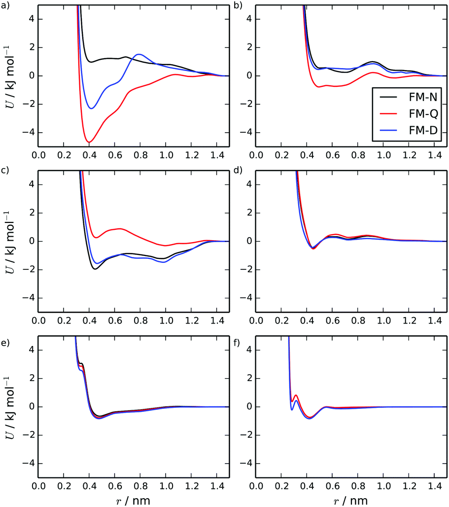

Fig. 2 HFM potentials calculated for the TP6EO2M/water system at 280 K, for the FM-N, FM-Q models and FM-D models. Showing the (a) C–C, (b) A–A, (c) C–A, (d) C–W, (e) A–W and (f) W–W coarse-grained potentials.

The unexpected shape of the potentials in the initial HFM model arises from the way that electrostatics are treated in the parametrisation process. It is assumed that (in the spirit of the MARTINI model) all coarse-grained beads are neutral. However, if the charges from the atomistic model were carried over to the coarse-grained model, the AI and CC beads would be neutral, but the AO and CO beads would have very small net charges of −0.2 e and + 0.2 e respectively. The electrostatic forces between the charged beads are included in the force matching and are effectively averaged over all the beads. This is the origin of the repulsive like interactions and the attractive unlike interactions. For TP6EO2M, this is less than optimal for two reasons: the electrostatic interactions should ideally apply only to the AO and CO beads (not all of the beads); and long-ranged electrostatic interactions are being implicitly included in the short-range vdW potentials, and any long-range effects are not being treated fully within the coarse-grained simulations.

This problem can be addressed within HFM by subtracting electrostatic interactions prior to the force matching. To do this, the electrostatic interactions arising from the mapping of the atomistic charges onto the coarse-grained beads were calculated for each frame of the mapped trajectory: giving the coarse-grained electrostatic forces for the system. The electrostatic forces were then subtracted from the reference forces (after the exclusion of intramolecular interactions), giving a new reference trajectory which did not include the coarse-grained electrostatic forces. The new reference was then used for force matching. Coarse-grained simulations of this model, FM-Q, included explicit charges on the AO (−0.2 e) and CO (+0.2 e) beads, and the electrostatic forces were calculated using the PME method. It should be noted that this method can only deal with electrostatic interactions between atoms which map onto charged beads; this neglects, for example, any electrostatic interactions involving water, which is neutral overall. However, this is still expected to be an improvement over the FM-N model.

The FM-Q model potentials are shown in Fig. 2. The interactions involving water are very similar to those in the FM-N model since the water beads are neutral in both models. However, the other interactions have changed significantly. The core–core interactions are now strongly attractive, the arm–arm is more weakly attractive and the core–arm interaction is overall slightly repulsive, but with two small attractive wells. Comparing the two models, the dominant influence of the implicit electrostatic interactions on the potentials of the FM-N model is apparent.

The two coarse-grained models exhibit subtly different behaviour in simulations. For both models, a stack of 10 molecules (2.5 wt%) remains stable over a 100 ns simulation. However, spontaneous self-assembly of the stack occurred over very different timescales (see ESI†). For FM-N, two short chromonic stacks assembled within 35 ns, with a 10-molecule stack forming within 100 ns. The FM-Q model assembled a 10-molecule chromonic stack within only 4 ns of simulation time. The difference between the two models was even more pronounced at a higher concentration (starting from 16 dispersed 16 TP6EO2M molecules at 4.7 wt%). Here, the FM-Q model formed a 16-molecule stack within 20 ns of simulation but over 100 ns the FM-N model was only able to form smaller stacks. These often formed and then disassembled later in the simulation, and side-on aggregation of two stacks was observed at several points in the simulated trajectory.

Partial radial distribution functions (RDFs), calculated for the FM-Q model, are plotted in Fig. 3. These show good overall agreement with the atomistic simulations but with significant quantitative differences where the coarse-grained model is unable to pick up the local structure. For example, for the C–W RDF (Fig. 3d), a difference in the atomistic and coarse-grained models is seen between 0.5 and 1.0 nm, where some of the local interactions have been lost. This region is less well-sampled than the others in the stacked configuration, as parts of the central core are usually hidden from water molecules.

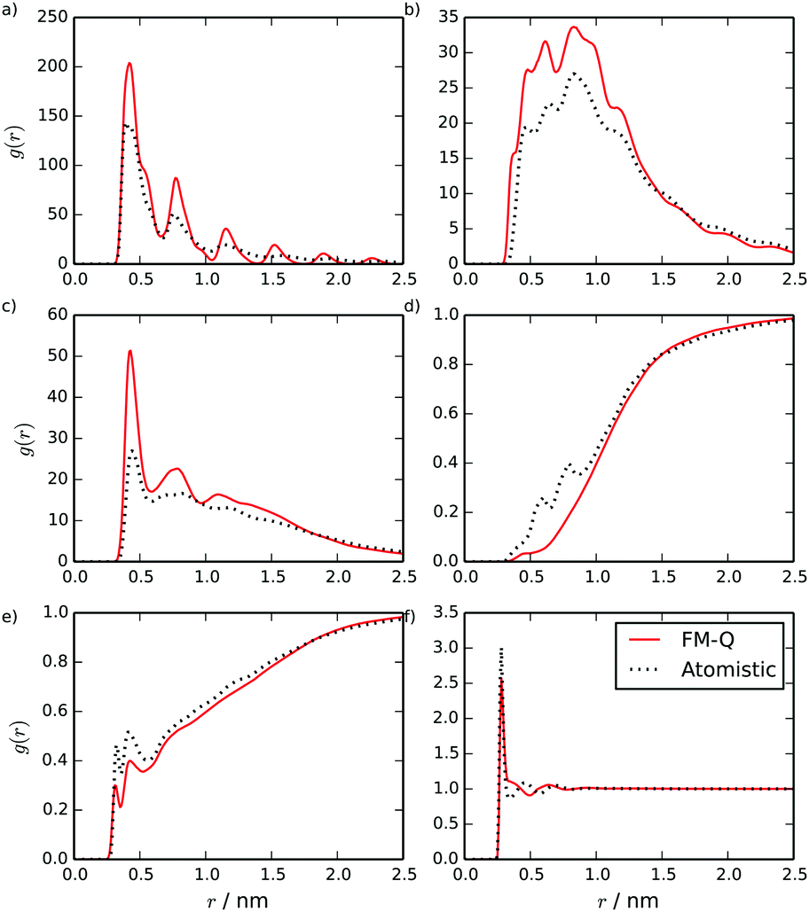Fig. 3 Site–site intermolecular RDFs calculated from a stack of 10 TP6EO2M molecules, using the FM-Q and atomistic models: (a) C–C, (b) C–A, (c) A–A, (d) C–W, (e) A–W and (f) W–W distributions.

Two distinct measures of the distance between two molecules in a stack have been used in previous studies of chromonic stacking. The first, d_com, is simply the distance between the centres of mass of two molecules, while the stacking distance, d_S, is the distance between the molecules projected along the average of the vectors normal to the cores of the two molecules. Using both measures together provides insights into the nature of the intermolecular stacking: distributions of the two quantities will show different features depending on, for example, whether there are offsets between adjacent molecules, or bends in the stack. These quantities were calculated for the TP6EO2M stack simulated using the atomistic and FM-Q models and are plotted in Fig. 4. The positions of the first peaks in both distributions are well represented by the FM-Q model; the model gives a d_S of 0.370 nm and d_com of 0.380 nm, which compare well to the atomistic values of 0.365 nm and 0.375 nm. However, the FM-Q distribution functions lack the tails that are present in the atomistic distributions at longer distances. These arise from flexibility in the molecular stacking leading to some bent configurations of a chromonic stack. Hence, long-distance behaviour is less well-represented within the coarse-grained model. The reason for this can be seen from calculated PMFs (see ESI†). For dimers, the free energy of association, Δ_associationG, calculated from the FM-Q PMF is −219 kJ mol⁻¹, which is more than 5 × the atomistic value.³⁹ (For the FM-N model, Δ_associationG is −180 kJ mol⁻¹; this is lower than the FM-Q value, but still significantly higher than the atomistic value.) Although it is known that there will be a contribution to the free energy of association arising from the density-dependence of the CG-potentials, it is still clear that the HFM approach leads to intermolecular potentials that significantly over-estimate the weak binding between chromonic molecules.

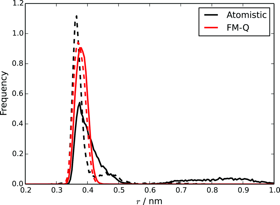Fig. 4 Distributions of d_S (dashed lines) and d_com (solid lines) for a stack of 10 TP6EO2M molecules, calculated using the atomistic and FM-Q models.

We briefly investigated two possible avenues to improve binding. Firstly, the use of a linear pressure correction for HFM⁴² was applied to the 10-molecule system. While this allowed the pressure to be well-represented in the 10-molecule CG simulation (and also transferred well to representing the pressure for chromonic dimer in water), the PMF calculated gave a Δ_associationG of −232 kJ mol⁻¹.

Secondly, we note from observation of the trajectories at d_com > 4.5 used for atomic PMFs, that one possible reason for the poor representation of the thermodynamics of dimer formation in HFM is that there are many intermolecular orientations, which are not usually sampled by the standard stack reference system. To try and account for this, we also tried an alternative reference simulation consisting of a mixture of shorter stacks in solution, where it was hypothesised that more distances and orientations would be sampled for TP6EO2M, including those contributing to the interactions between the stacks. The starting structure for this reference was 50 monomers dispersed in water, which were allowed to assemble into short stacks over 20 ns. The HFM model calculated using this reference, referred to as FM-D (see Fig. 2 for the CG interaction potentials), produces a CG model where the core–core interactions are substantially reduced in strength of attraction, while other interactions are similar. Simulation of this model over long times leads to a mixture of monomers and short stacks (similar to the reference simulation), and simulation of a longer stack leads to fragmentation into shorter fragments.

The results highlight the difficulties of making a truly representative bottom-up model for chromonics based on an atomic reference. For the coarse-grained model to be truly representative of the system, it must be able to capture even those configurations which are rarely seen. A possible future solution to this could be a multi-state parametrisation, where both a stack and a dispersed system are used as references, along with local-density (L-D) potentials,^68–70 which in this case could be used as a metric for whether a molecule is a monomer, in the middle of a stack or at the stack end (altering the interaction with other molecules accordingly). A related approach has been used for a hydrophobic polymer, where the L-D potential described whether a particular region of a polymer was part of an aggregate.⁷¹

3.2 MARTINI 3

Using a starting configuration of 10 TP6EO2M molecules dispersed in water, simulation of the four MARTINI 3 models for TP6EO2M reveals very different behaviour depending on the parameters used for the AI and AO beads. Fig. 5 shows snapshots taken after 100 ns of simulation for each of the models. The N0 and N0a models both give a 10 molecule chromonic stack in that time frame. The N1 model gives two shorter chromonic stacks, while the N1a model gives two short stacks and one monomer.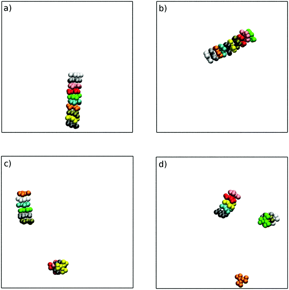

Fig. 5 Final configurations from 100 ns simulations of 10 TP6EO2M molecules in water, using the (a) N0, (b) N0a, (c) N1 and (d) N1a models. For clarity, only the aromatic core beads are shown, and are coloured by molecule.

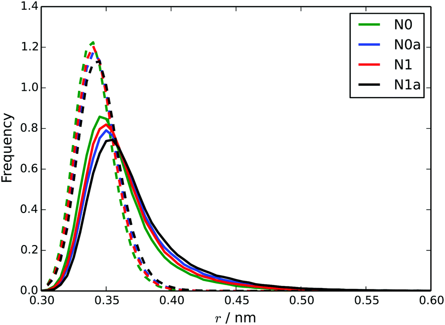
Starting from a pre-assembled stack of 10 TP6EO2M molecules, the chromonic stack was found to be stable over 100 ns for all 4 models. Fig. 6 shows d_com and d_S distributions calculated for the nearest neighbours in the stack. The stacking distances are in quite good agreement with the atomistic data (Fig. 4) but noting that the d_com values are shifted to slightly higher values compared to d_S, indicating slight offsets between adjacent molecules in the stack. The d_com distribution has a long tail compared to the HFM model of Fig. 4, indicating that the MARTINI 3 stacks have a similar degree of flexibility as the atomistic model. Here, the MARTINI 3 models are less tightly anchored in stacks, leading to greater stack flexibility. The models do exhibit some variation in their stacking distance, despite using the same bead type for the core. This may be rationalised in terms of solubility; the models with more soluble A beads have a larger d_S, allowing for greater solvation of the hydrophilic arms.

Fig. 6 Distributions of d_com (solid lines) and d_S (dotted lines) for each of the four MARTINI 3 models.

Fig. 7 shows a comparison between site–site intermolecular RDFs from MARTINI 3 models and the atomistic simulations. The CG models capture the key structural features of the atomistic model, albeit with sharper peaks in the RDFs arising from the fact that MARTINI sites are at the centre of beads and the atomistic results use centres of mass of beads (which can fluctuate slightly for each bead).

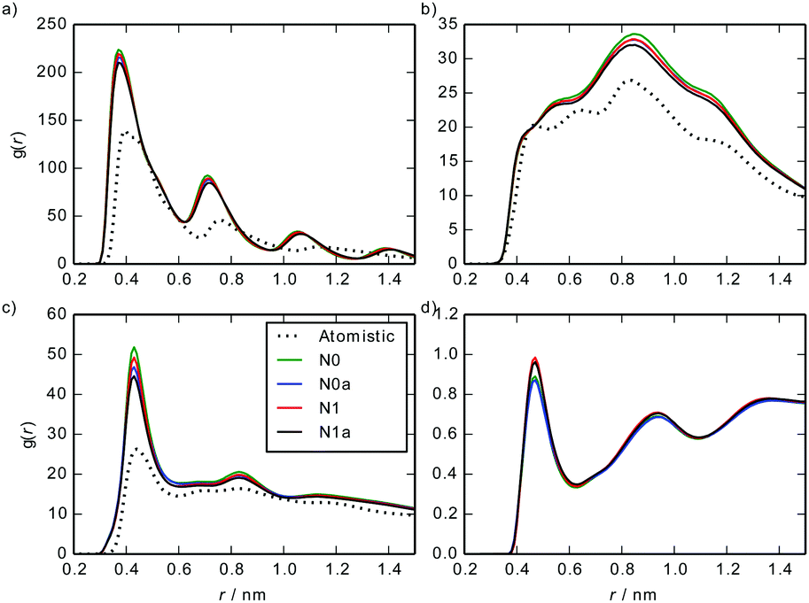Fig. 7 Site–site intermolecular RDFs calculated from a stack of 10 TP6EO2M molecules, using the MARTINI 3 and atomistic models: (a) C–C, (b) C–A, (c) A–A, (d) A–W.

In the ESI† we include additional information about the arrangements of molecules within chromonic stacks. For all models, the distribution of pairwise tilt angles is strongly peaked around zero tilt. Adjacent molecules within a stack are staggered so that chains do not directly overlap. This increases solvation of chains but also allows a larger preferred distance between hydrophilic chains in comparison to the aromatic cores. For the atomistic model, the distribution function for the azimuthal angle for adjacent cores in a stack is peaked at exactly 60, 180 and 300 degrees (corresponding to three identical staggered arrangements of adjacent cores) whereas each of these peaks is split into two within the MARTINI 3 model, due to the packing effects of the two CO beads at the edge of each outer aromatic ring. Hence, the choice of mapping means that the azimuthal distribution function cannot be exactly reproduced within the coarse-grained framework.

The PMFs calculated using the MARTINI 3 models are as shown in Fig. 8. The Δ_associationG values from these PMFs, for the N0, N1, N0a and N1a models respectively, are: −46.3 ± 1.5, −36.7 ± 1.5, −42.6 ± 1.5 and −32.4 ± 1.4 kJ mol⁻¹. These all represent a significant improvement over the HFM models, in terms of reproducing the atomistic free energy for dimer association (40.7 kJ mol⁻¹) calculated by Akinshina et al.³⁹ The differences between the PMFs are consistent with the behaviour of the models in simulations i.e., N0 and N0a models have slightly deeper potential wells. All of the CG PMFs have a very small barrier to association (2–3 kJ mol⁻¹). The origin of this barrier is from solvation. As two TP6EO2M molecules approach each other, they are initially fully solvated by water but at around 1.5–1.7 nm as the two molecules start to interact there is insufficient room between the two molecules for all of the beads to be fully solvated for all orientations. However, the attraction between the TP6EO2M cores is too small to cancel this out at these long distances.

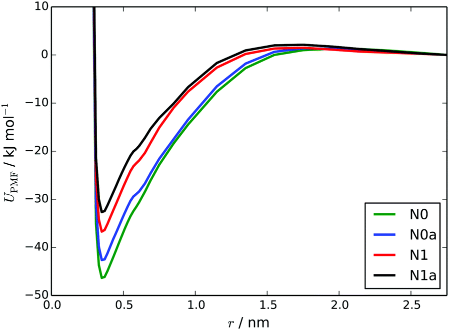Fig. 8 PMFs for the separation of a TP6EO2M dimer, calculated using the four MARTINI 3 models.

3.3 Liquid crystal phases from MARTINI 3

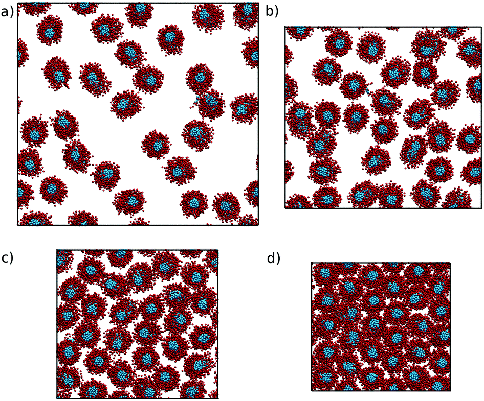
To test the ability of these models to form self-assembled chromonic phases, a large simulation box was set up containing 1000 TP6EO2M molecules with random positions and orientations, solvated by 36 876 MARTINI water beads; this corresponds to a concentration of 26.1% by weight, which is in the nematic region of the TP6EO2M phase diagram at 280 K. An atomistic representation of this system would consist of 580 512 atoms, the simulation of which would not be feasible without very large computational resources. However, using 72 CPU cores, the MARTINI 3 model achieved speeds of around 35 ns per day.

These large scale simulations provide further insight into the representability of the four MARTINI 3 models. All of the models produced chromonic stacks during the simulations. However, the N0 and N0a models, which performed well in the small-scale simulations, led to phase separation at this concentration, forming distinct liquid TP6EO2M and water regions. The N1 and N1a models, on the other hand, formed long chromonic stacks which were fully solvated in water. Representative simulation snapshots from the N0 and N1 models are shown in Fig. 9.

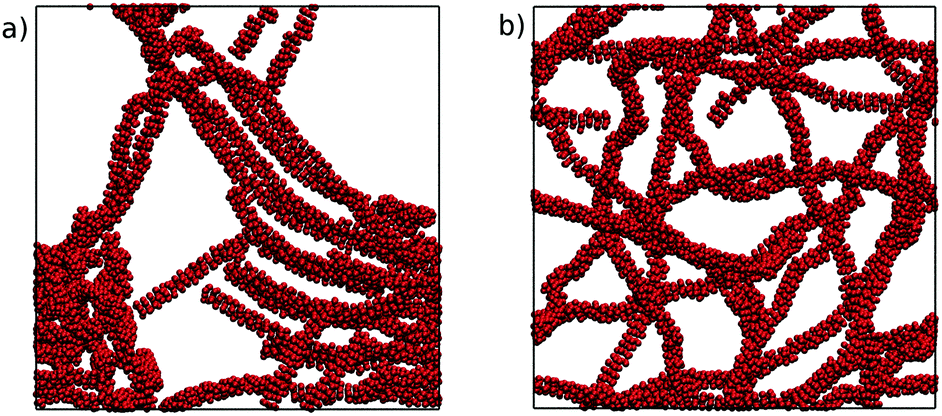Fig. 9 Final configurations after 500 ns of simulation from a starting point of 1000 TP6EO2M molecules in water, using the (a) N0 and (b) N1 MARTINI 3 models.

The difference in behaviour between the models can be attributed to the solubility of the beads used for the hydrophilic arms. The N0 and N0a beads are insufficiently soluble so that when multiple long stacks are modelled, they preferentially aggregate together. The higher solubility of the N1 and N1a beads prevents this from happening. These results highlight the difficulties in parametrising models for hierarchical systems like chromonic liquid crystals; a model which is representative at one scale may not perform as well at another scale and the balance between core–core, core–arm, core–water and arm–water interactions all subtly change association behaviour.

Even though the formation of chromonic stacks was observed in the first few nanoseconds of simulation of the N1 and N1a models, the self-assembly of these stacks into the nematic phase was not seen over 500 ns of simulation. The evolution of the nematic order parameter, S_nematic, shows the system order parameter rarely fluctuates above 0.2. Here, many of the chromonic stacks are observed to be continuous over periodic boundary conditions and are tangled up with other stacks. For the nematic phase to be formed, these stacks would first need to break and disentangle themselves. Given the speed with which chromonic stacks are formed and the high free energy driving force for molecular stacking, it is extremely unlikely that this will be observed within a reasonable simulation timescale using standard molecular dynamics without the use of an alignment field (e.g., magnetic field) or shear.

However, to look at potential nematic (N) and hexagonal (M) phases, an untangled hexagonal columnar system was preassembled and allowed to evolve and observed for different concentrations. Here, starting structures were constructed by placing 30 columns with 30 TP6EO2M molecules each in a hexagonal arrangement within a cuboidal simulation box and solvated with varying amounts of MARTINI 3 water corresponding to TP6EO2M/water concentrations of 27.1, 39.4, 55.8 and 71.4 wt%. All starting structures had the same initial volume, so the volumes of the boxes were allowed to equilibrate before any data was gathered, employing semi-isotropic pressure coupling to allow the cross-section of the nematic phase and the lengths of the columns to change independently. The system densities equilibrated within 200 ps for all of the concentrations, and remained stable throughout the simulations; equilibrated densities are given in Table 2. Each system was simulated for a total of 500 ns to look for the transition to the hexagonal phase.

Table 2 TP6EO2M/water concentrations studied and their densities, nematic order parameters and the chromonic phases formed

Concentration/wt%	ρ/kg m^−3	S nematic (N1a)	LC phase
27.1	1093	0.914	N
39.4	1129	0.915	N
55.8	1181	0.922	M
71.4	1238	0.931	M

---

These simulations provided further insights into which bead type best represents the arm beads. Here, the N1 and N1a models exhibited significantly different behaviour. Using the N1 model, there was a tendency at higher concentrations (∼55 wt%) for the stacks to form small clusters of columns with ethylene oxide arms in close proximity, with stacks that were not fully solvated (see ESI†). At these higher concentrations, the N1a model shows the M (C_H) phase as predicted by the phase diagram, while the formation of clusters of columns by the N1 model disrupts the formation of regular hexagonal packing. Despite the excellent performance of the N1 model in simulating the self-assembly of short stacks and close agreement to atomistic and experimental values of Δ_associationG, it is far less representative at higher concentrations.

The N1a model was therefore used for more detailed analysis of the system across the concentration range. The nematic order parameter, S_nematic, was calculated for each concentration to quantify the orientational order of each system, and the values are shown in Table 2. In each case, S_nematic is greater than 0.9, showing long-range orientational order. The value increases slightly with TP6EO2M concentration; which is expected, as increased concentration leads to closer packing of the columns.

Two-dimensional pair distribution functions are shown in Fig. 10, along with the configurations after 500 ns showing the cross-section of the nematic/hexagonal phase in Fig. 11. The two lower concentrations show clear liquid behaviour in two dimensions; combined with the S_nematic values, this indicates the nematic phase. Between 39.4% and 55.8%, there is a clear transition from liquid-like to hexagonal ordering in close agreement with experiment.^7,36

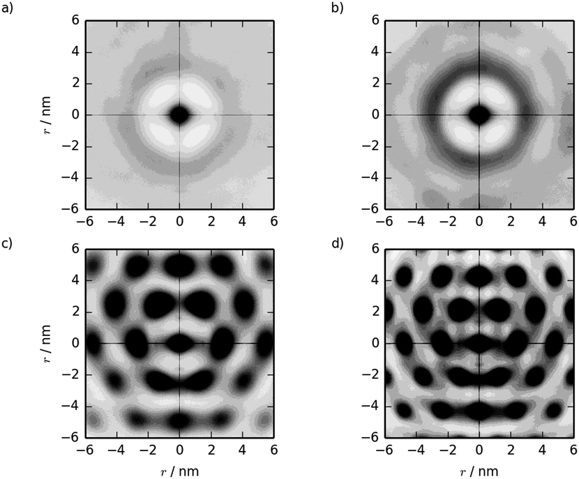Fig. 10 Two dimensional g(u,v) from simulations of pre-assembled TP6EO2M columnar phases at concentrations of (a) 27.1, (b) 39.4, (c) 55.8 and (d) 71.4 wt%.

Fig. 11 Configurations taken after 500 ns of simulations of the N1a model, starting from pre-assembled columnar structures at (a) 27.1, (b) 39.4, (c) 55.8 and (d) 71.4 wt%.

It should be noted that these simulations are effectively modelling a series of infinitely long stacks. A system with a distribution of sizes might be expected to behave slightly differently as the presence of short stacks in the system may disrupt hexagonal packing, resulting in a slightly more disordered M phase. Despite this limitation, the results here show that the MARTINI 3 force field is well-suited to modelling the concentration dependence of the TP6EO2M/water phase diagram.

4 Conclusions

We have investigated the use of coarse-grained models to study a nonionic chromonic liquid crystal, TP6EO2M. Chromonic systems are extremely challenging to study due to the combination of self-assembly in solution, self-organisation of chromonic stacks, the presence of both enthalpic and entropic driving forces for self-assembly, and the subtle balance of hydrophobic and hydrophilic interactions of different groups. The latter, in particular, places chromonic mesogens delicately balanced between individually dispersed molecules and phase-separated (or crystallized) aggregates.

We find that the hybrid force matching method is successful in reproducing chromonic stacks in solution. However, the binding between CG molecules is found to be very high, reflecting the lack of transferability between state points that occurs with force matching methods. In future, it will be interesting to see whether CG potentials that can adjust to their environment (such as density-dependent CG potentials) could be employed to improve transferability in chromonics and similar systems.

We also tested MARTINI models for TP6EO2M. These are also found to be sensitive to the hydrophilic–hydrophobic balance of different parts of the molecule in solution. However, we were able to demonstrate a model that shows good self-assembly behaviour in solution and can also be used in the nematic (N) and hexagonal (M) phases. For such a simple CG model this demonstrates a high degree of transferability over a substantial concentration range across the phase diagram, opening up possibilities of using these models to study a wide range of drug and dye molecules that show chromonic-type assembly in solution.

Conflicts of interest

There are no conflicts to declare.

Acknowledgements

The authors would like to acknowledge the support of Durham University for the use of its HPC facility, Hamilton. T. D. P. would like to thank EPSRC for the award of a studentship (grant EP/M507854/1, award reference 1653213). M. R. W. and M. W. would like to thank the UK research council, EPSRC, for funding under grants EP/J004413/1 and EP/P007864/1.

Notes and references

1. J. Lydon, Liq. Cryst., 2011, 38, 1663–1681.
2. J. Lydon, J. Mater. Chem., 2010, 20, 10071–10099.
3. P. J. Collings, J. N. Goldstein, E. J. Hamilton, B. R. Mercado, K. J. Nieser and M. H. Regan, Liq. Cryst. Rev., 2015, 3, 1–27.
4. F. Chami and M. R. Wilson, J. Am. Chem. Soc., 2010, 132, 7794–7802.
5. H. Sidky and J. K. Whitmer, J. Phys. Chem. B, 2017, 121, 6691–6698.
6. O. M. M. Rivas and A. D. Rey, Mol. Syst. Des. Eng., 2017, 2, 223–234.
7. A. Masters, Liq. Cryst. Today, 2016, 25, 30–37.
8. C. J. Bottrill, PhD thesis, UMIST, 1999.
9. R. Thind, M. Walker and M. R. Wilson, Adv. Theory Simul., 2018, 1, 1800088.
10. M. Walker and M. R. Wilson, Soft Matter, 2016, 12, 8588–8594.
11. N. Hartshorne and G. Woodard, Mol. Cryst. Liq. Cryst., 1973, 23, 343–368.
12. T. K. Attwood and J. E. Lydon, Mol. Cryst. Liq. Cryst., 1984, 108, 349–357.
13. E. E. Jelley, Nature, 1937, 139, 631.
14. G. J. T. Tiddy, D. L. Mateer, A. P. Ormerod, W. J. Harrison and D. J. Edwards, Langmuir, 1995, 11, 390–393.
15. W. J. Harrison, D. L. Mateer and G. J. T. Tiddy, J. Phys. Chem., 1996, 100, 2310–2321.
16. T. L. Crowley, C. Bottrill, D. Mateer, W. J. Harrison and G. J. T. Tiddy, Colloids Surf., A, 1997, 129–130, 95–115.
17. T. Schneider and O. Lavrentovich, Langmuir, 2000, 16, 5227–5230.
18. D. J. Edwards, J. W. Jones, O. Lozman, A. P. Ormerod, M. Sintyureva and G. J. T. Tiddy, J. Phys. Chem. B, 2008, 112, 14628–14636.
19. M. R. Tomasik and P. J. Collings, J. Phys. Chem. B, 2008, 112, 9883–9889.
20. A. Ryzhakov, T. Do Thi, J. Stappaerts, L. Bertoletti, K. Kimpe, A. R. S. Couto, P. Saokham, G. Van den Mooter, P. Augustijns and G. W. Somsen, et al. , J. Pharm. Sci., 2016, 105, 2556–2569.
21. H.-S. Park and O. D. Lavrentovich, Lyotropic chromonic liquid crystals: emerging applications, in Liquid Crystals Beyond Displays: Chemistry, Physics, and Applications, ed. Q. Li, Wiley Online Library, 2012, pp. 449–484.
22. S.-W. Tam-Chang and L. Huang, Chem. Commun., 2008, 1957–1967.
23. S.-W. Tam-Chang, W. Seo, I. K. Iverson and S. M. Casey, Angew. Chem., Int. Ed., 2003, 42, 897–900.
24. I. K. Iverson, S. M. Casey, W. Seo, S.-W. Tam-Chang and B. A. Pindzola, Langmuir, 2002, 18, 3510–3516.
25. H. J. Kim, W.-B. Jung, H. S. Jeong and H.-T. Jung, J. Mater. Chem. C, 2017, 5, 12241–12248.
26. M. Lavrentovich, T. Sergan and J. Kelly, Liq. Cryst., 2003, 30, 851–859.
27. C. Peng and O. D. Lavrentovich, Soft Matter, 2015, 11, 7257–7263.
28. P. Van der Asdonk and P. H. Kouwer, Chem. Soc. Rev., 2017, 46, 5935–5949.
29. C. Rodriguez-Abreu, C. A. Torres and G. J. Tiddy, Langmuir, 2011, 27, 3067–3073.
30. S. Zhou, A. Sokolov, O. D. Lavrentovich and I. S. Aranson, Proc. Natl. Acad. Sci. U. S. A., 2014, 111, 1265–1270.
31. C. Peng, T. Turiv, Y. Guo, Q.-H. Wei and O. D. Lavrentovich, Science, 2016, 354, 882–885.
32. T. D. Potter, J. Tasche, E. L. Barrett, M. Walker and M. R. Wilson, Liq. Cryst., 2017, 1–11.
33. M. Walker and M. R. Wilson, Mol. Cryst. Liq. Cryst., 2015, 612, 117–125.
34. N. Boden, R. J. Bushby and C. Hardy, J. Phys., Lett., 1985, 46, 325–328.
35. N. Boden, R. J. Bushby, C. Hardy and F. Sixl, Chem. Phys. Lett., 1986, 123, 359–364.
36. N. Boden, R. J. Bushby, L. Ferris, C. Hardy and F. Sixl, Liq. Cryst., 1986, 1, 109–125.
37. R. E. Hughes, S. P. Hart, D. A. Smith, B. Movaghar, R. J. Bushby and N. Boden, J. Phys. Chem. B, 2002, 106, 6638–6645.
38. Z. H. Al-Lawati, B. Alkhairalla, J. P. Bramble, J. R. Henderson, R. J. Bushby and S. D. Evans, J. Phys. Chem. C, 2012, 116, 12627–12635.
39. A. Akinshina, M. Walker, M. R. Wilson, G. J. T. Tiddy, A. J. Masters and P. Carbone, Soft Matter, 2015, 11, 680–691.
40. M. Walker, A. J. Masters and M. R. Wilson, Phys. Chem. Chem. Phys., 2014, 16, 23074–23081.
41. P. C. Souza, S. Thallmair, P. Conflitti, C. Ramrez-Palacios, R. Alessandri, S. Raniolo, V. Limongelli and S. J. Marrink, Nat. Commun., 2020, 11, 1–11.
42. T. D. Potter, J. Tasche and M. R. Wilson, Phys. Chem. Chem. Phys., 2019, 21, 1912–1927.
43. W. G. Noid, J.-W. Chu, G. S. Ayton, V. Krishna, S. Izvekov, G. A. Voth, A. Das and H. C. Andersen, J. Chem. Phys., 2008, 128, 244114.
44. C. Peter and K. Kremer, Faraday Discuss., 2010, 144, 9–24.
45. C. Peter and K. Kremer, Soft Matter, 2009, 5, 4357.
46. R. G. Edwards, J. Henderson and R. L. Pinning, Mol. Phys., 1995, 86, 567–598.
47. L. Lu, S. Izvekov, A. Das, H. C. Andersen and G. A. Voth, J. Chem. Theory Comput., 2010, 6, 954–965.
48. Martini 3 open-beta, http://cgmartini.nl/index.php/martini3beta, accessed July 2018.
49. S. Pronk, S. Pall, R. Schulz, P. Larsson, P. Bjelkmar, R. Apostolov, M. R. Shirts, J. C. Smith, P. M. Kasson, D. van der Spoel, B. Hess and E. Lindahl, Bioinformatics, 2013, 29(7), 845–854.
50. W. L. Jorgensen and J. Tirado-Rives, J. Am. Chem. Soc., 1988, 110, 1657–1666.
51. S. Nosé, J. Chem. Phys., 1984, 81, 511–519.
52. W. G. Hoover, Phys. Rev. A: At., Mol., Opt. Phys., 1985, 31, 1695–1697.
53. M. Parrinello and A. Rahman, J. Appl. Phys., 1981, 52, 7182–7190.
54. N. J. H. Dunn, K. M. Lebold, M. R. DeLyser, J. F. Rudzinski and W. Noid, J. Phys. Chem. B, 2018, 122, 3363–3377.
55. V. Rühle, C. Junghans, A. Lukyanov, K. Kremer and D. Andrienko, J. Chem. Theory Comput., 2009, 5, 3211–3223.
56. S. J. Marrink, H. J. Risselada, S. Yefimov, D. P. Tieleman and A. H. de Vries, J. Phys. Chem. B, 2007, 111, 7812–7824.
57. L. Monticelli, S. K. Kandasamy, X. Periole, R. G. Larson, D. P. Tieleman and S. J. Marrink, J. Chem. Theory Comput., 2008, 4, 819–834.
58. D. H. de Jong, G. Singh, W. F. D. Bennett, C. Arnarez, T. A. Wassenaar, L. V. Schäfer, X. Periole, D. P. Tieleman and S. J. Marrink, J. Chem. Theory Comput., 2013, 9, 687–697.
59. S. J. Marrink and D. P. Tieleman, Chem. Soc. Rev., 2013, 42, 6801–6822.
60. C. A. López, A. J. Rzepiela, A. H. de Vries, L. Dijkhuizen, P. H. Hünenberger and S. J. Marrink, J. Chem. Theory Comput., 2009, 5, 3195–3210.
61. G. Rossi, L. Monticelli, S. R. Puisto, I. Vattulainen and T. Ala-Nissila, Soft Matter, 2011, 7, 698–708.
62. H. Lee, A. H. de Vries, S. J. Marrink and R. W. Pastor, J. Phys. Chem. B, 2009, 113, 13186–13194.
63. L. I. Vazquez-Salazar, M. Selle, A. de Vries, S. J. Marrink and P. C. Souza, Green Chem., 2020 10.1039/D0GC01823F.
64. R. Hashim, G. R. Luckhurst and S. Romano, Mol. Phys., 1985, 56, 1217–1234.
65. M. R. Wilson, J. Chem. Phys., 1997, 107, 8654–8663.
66. H. Wang, C. Junghans and K. Kremer, Eur. Phys. J. E: Soft Matter Biol. Phys., 2009, 28, 221–229.
67. A. Lyubartsev, A. Mirzoev, L. Chen and A. Laaksonen, Faraday Discuss., 2009, 144, 43–56.
68. M. R. DeLyser and W. G. Noid, J. Chem. Phys., 2017, 147, 134111.
69. T. Sanyal and M. S. Shell, J. Phys. Chem. B, 2018, 122, 5678–5693.
70. J. Jin and G. A. Voth, J. Chem. Theory Comput., 2018, 14, 2180–2197.
71. T. Sanyal and M. S. Shell, J. Chem. Phys., 2016, 145, 034109.

---

Footnote

† Electronic supplementary information (ESI) available: Intramolecular components of the coarse-grained force field, hybrid force matching intermolecular potentials (C–C interaction), snapshot configurations showing self-assembly in solution, structural data for chromonic stacks, PMFs for TP6EO2M dimers, snapshots from liquid crystal phases. See DOI: 10.1039/d0sm01157f

---