 Open Access Article
The journey of a single polymer chain to a nanopore
Navid
Afrasiabian
 *a and
Colin
Denniston
 ab
ab
aDepartment of Applied Mathematics, University of Western Ontario, London, Canada. E-mail: nafrasia@uwo.ca
bDepartment of Physics and Astronomy, University of Western Ontario, London, Canada. E-mail: cdennist@uwo.ca
First published on 11th September 2020
Abstract
For a polymer to successfully thread through a nanopore, it must first find the nanopore. This so-called capture process is typically considered as a two-stage operation consisting of the chain being delivered at the entrance of the nanopore and then insertion of one of the ends. Studying molecular dynamics-lattice Boltzmann simulations of the capture of a single polymer chain under pressure driven hydrodynamic flow, we observe that the insertion can be essentially automatic with no delay for the ends searching for the nanopore. The deformation of the chain within the converging flow area and also, the interplay between the chain elastic forces and the hydrodynamic drag play an important role in the capture of the chain by the nanopore. Along the journey to the nanopore, the chain may form folded shapes. The competition between the elastic and hydrodynamic forces results in unraveling of the folded conformations (hairpins) as the chain approaches the nanopore. Although the ends are not the only monomers that can thread into the nanopore, the unraveling process can result in much higher probability of threading by the ends.
1 Introduction
Due to its pivotal role in many biological systems and processes, like protein transport through cell membranes or virus injection,1,2 polymer translocation has attracted a lot of attention from physics to biology communities. With the emergence of fast and single-molecule sequencing techniques, and the hope of creating even cheaper and faster methods,3–5 the importance of understanding the motion of a single polymer chain while it passes through a nano-scale pore has grown even more significant in the past two decades.6–8 For the translocation to take place, the chain must move from the ambient environment far from the nanochannel to its entrance and then thread through. This process can happen in the absence or presence of external forces. In this paper, we investigate the dynamics of a single polymer chain in its journey to the nanopore in the presence of pressure-driven hydrodynamic flow and describe the effect such a flow has on the capture process.Early theoretical studies on unbiased translocation started with the assumption that the threading process is slow enough that segments on both sides of the pore can effectively be modeled as in-equilibrium chains anchored at the pore.9,10 This allows the application of a number of equilibrium scaling arguments. For a polymer chain to translocate through a nanopore, it must travel a distance larger than its radius of gyration. Considering that the translocating chain is restricted to travel this distance through a small pore, one may expect this process to take longer than the Rouse relaxation time of the free chain. Chuang et al. pointed out that the early studies were not consistent with this limitation11 and they came to the conclusion that the polymer cannot equilibrate during translocation. Hence, the process must be a non-equilibrium one. As their Monte Carlo (MC) simulations illustrated, the dynamics of translocation is anomalous. Anomalous dynamics were observed by other groups as well.12,13 Chuang, Kantor, and Kardar set up MC simulations with an extra condition on the end that goes through first, requiring the end to move forward. As this causes a change in the scaling behaviour of the translocation time (τ), Luo et al. and Huopaniemi et al. instead placed the chain initially halfway through the nanopore and measured an escape time without the need for artificial conditions on the chain end.14,15 With no external force in unbiased translocation, τ only scales with the chain length (N),
| τ ∼ Nα | (1) |
In the case of biased translocation, the effect of the driving force f must also be considered in the scaling relation,
| τ ∼ Nα/fγ | (2) |
In a pioneering work, Sakaue considered translocation as the process during which a tension created by the forces in the nanopore propagates along the polymer backbone.28 In this model, a tension front was defined which shows how far the tension has travelled along the chain. The chain consists of the part close to the nanopore which feels the force of the nanopore and the rear part which is still relaxed. Sakaue described the influenced part of the chain using a diverging blob model introduced by Pincus.33 In their work, however, the polymer is positioned at the entrance of the nanopore and the fact that the chain might already be stretched out as it reaches the pore was not discussed. Pre-translocation deformations were observed for a voltage-driven capture by Farahpour et al.34 They studied a single stranded DNA translocation through a solid-state pore using multiscale simulations and found out that the chain deforms as a result of the non-uniform electric field. In the present work, we see a similar behaviour, however, for a neutral chain in a pressure-driven hydrodynamic flow.
A hydrodynamic flow can facilitate polymer insertion and translocation. Daoudi and Brochard showed that a critical flow rate is required for forward drag forces from the flow to overcome the chain's entropic retraction and guarantee insertion.35 They found the critical current depends linearly on temperature, and inversely on the solvent viscosity. Sakaue et al. showed that the dynamics of insertion, also known as suction, is determined by the entry of a segment of the size of the pore and is independent of branching.36 These findings were later confirmed by Markestenijn et al. through multiscale simulations.37 The main focus of such studies have mostly been on the translocation step. The effect of hydrodynamic flow on polymer capture has not been investigated as much.
Experiments using fast sequencing techniques and nanopore sensing prefer single-file over folded threading of the pore as folds result in secondary current drops which make analyzing the data and distinguishing between different effects difficult. Single-file insertion is actually found to be surprisingly common.38 In a recent work, Ermann et al. showed that it is possible to control formation of these folded shapes by adjusting the electrolyte concentration.39 Although their method enhances the single-file capture, it comes with some caveats. For example, decreasing the ionic strength may also reduce the translocation time resulting in a drop in resolution.
Alternatively, extension induced by hydrodynamic flow, as we observe here, raise the hope for development of methods which promote single-file capture without these limitations. In Section 2 we present the system setup, the polymer and fluid model, and the multiscale simulation method. Section 3 consists of the results collected from 85 realizations for polymer chains of length 32 and 64 monomers, and the related theoretical arguments. We sum up our paper with a short summary and conclusion in Section 4.
2 Methodology
In pursuit of understanding the universal features of polymer translocation, especially the effect of hydrodynamics on the capture process, we studied the dynamics of a general coarse-grained polymer molecule immersed in a Lattice Boltzmann (LB) fluid. The simulations used the open source Molecular Dynamics software LAMMPS.40Fig. 1 shows a snapshot of our system. In our polymer model, the monomers were connected by Finitely Extensible Nonlinear Elastic (FENE) bonds41 with potential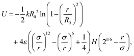 | (3) |
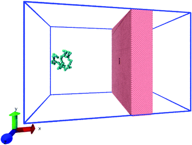 | ||
| Fig. 1 The system consists of a coarse-grained polymer chain (jade) and the a solid-state nanopore which is made out of a hole in a solid-state wall (pink). The boundaries of the system are periodic (blue lines). The visual molecular dynamics (VMD) software is used for visualizing the system.51 | ||
The interaction of a polymer chain with the solvent in which it is suspended plays an important role in the dynamics of the chain. In order to capture this hydrodynamic interaction, we embed our polymer chain in a fluctuating LB fluid. The LB algorithm, implemented into LAMMPS by Mackay et al.,43 provides both the hydrodynamic forces and random thermal agitation. In this method, the fluid is reproduced by solving an approximation to the Boltzmann transport equation with a single relaxation time on a lattice,
 | (4) |
As we will discuss in greater depth later, we are interested in the possible deformations of the polymer chain as it approaches the nanopore and therefore, it is essential to compare the polymer conformation to its equilibrium conformation. A good measure of the polymer shape is the radius of gyration (RG) of the chain which is defined as,
 | (5) |
| RF ≈ (0.5σ)Nν | (6) |
In the main simulations, the fluid interacted with both the polymer chain and the nanopore wall. The nanopore is a hole of size 10 nm × 4 nm × 4 nm through an atomistic wall. The width of the nanopore is wide enough to allow for polymer translocation either single-file or with one fold. The wall and the polymer chain interact with each other with a purely repulsive LJ force and the velocity of the fluid at the wall is zero (no-slip condition). The simulation box is of size 80 nm × 52 nm × 52 nm with periodic boundary in all directions. In order to generate independent results, each realization is run with different random seed generator and initial chain conformation. However, the centre of mass of the chain is initially placed at a specific distance from the wall, x − xent ≈ 4RF and in the central area of the box 16 nm < y < 36 nm, 16 nm < z < 36 nm. Fig. 1 shows a snapshot of the initial state of the system and Fig. 2a demonstrates the flow field in terms of streamlines in the absence of thermal noise. The force driving the flow arises from a pressure jump (Δp) at the boundaries in the x-direction (flow direction). The resulting flow is non-uniform and converging/diverging as it enters/exits the nanochannel. The data shown in the subsequent graphs are the average result of 55 realizations for the 64-mer chain and 30 realization for the 32-mer unless mentioned otherwise.
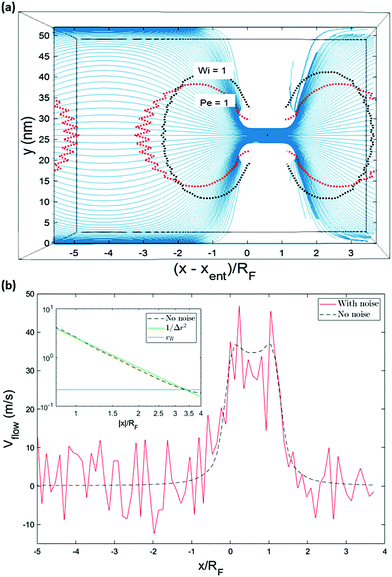 | ||
| Fig. 2 The solvent surrounding the polymer is a LB fluid. In (a), streamlines in a cross-section of the flow for a system without random noise is visualized in Paraview.52 The general features of the flow field are expected to be similar to the time-averaged flow in the case of a system with thermal noise. (b) Shows the velocity of the fluid plotted versus the fluid position along an axis going through the pore. The inset shows the velocity as a function of the absolute value of the relative position of the fluid (blue line shows the fluid velocity corresponding to a Pe number of one). The velocity increases in inverse-square fashion approaching the nanochannel. | ||
3 Results and discussion
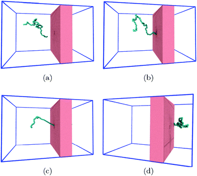
Polymer translocation is the process of a single polymer chain going through a biological or solid-state pore, the latter in our case, that is the same size or smaller than the radius of gyration of the chain. The polymer's journey starts in the bulk and far from the hole, as shown in Fig. 1. In this region, the flow field is uniform and weakly-driven, as illustrated in Fig. 2a by the uniform streamlines. The change in the system cross-section from the bulk region to the nanopore results in a converging flow with growing strength, due to conservation of mass and momentum, approaching the nanochannel. Fig. 2b shows the velocity of the fluid as a function of position for systems with and without thermal noise. The inset is a logarithmic graph of the velocity as the fluid approaches the nanopore. As this graph shows, the velocity increases like 1/|rpore|2, where |rpore| is the distance from the pore, as expected based on the fact that all the streamlines from the bulk must converge into the pore as it is the only exit. Daoudi and Brochard's critical current at the pore required for insertion is Jc ∼ kBT/η = 41 nm3 ns−1, where η is the fluid viscosity. The flow velocity at the pore in our system is high enough so that the current at the pore is more than an order of magnitude larger than this. As such, once the polymer gets close enough to the pore, it is essentially guaranteed to translocate. The main focus here is on what happens to the polymer as it moves from far away to close proximity to the pore.The converging flow induces extensions in the polymer, as can be seen in Fig. 3a. When a segment of the chain arrives at the entrance of the nanopore, Fig. 3b, the translocation starts. We will refer to the monomer that threads into the nanopore before any other monomer as the front monomer while the monomer which is ahead of other monomers at any given time is referred to as the leading monomer. The front monomer can be one of the ends (single-file conformation), as in Fig. 3b, or any other monomer along the chain (hairpin conformation), as shown in Fig. 4.38,53 During the translocation, monomers thread through the nanochannel from the cis side, where the chain originates, to the trans side, where the chain translocates to, as shown in Fig. 3c until the whole chain arrives at the trans side, as in Fig. 3d. In the rest of this section, we discuss how a non-uniform hydrodynamic flow affects the capture of a single polymer chain through the results obtained from MD-LB simulations.
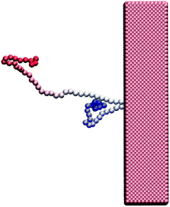 | ||
| Fig. 4 A hairpin structure threading the nanopore. The polymer is shown with gradient colouring to distinguish the ends from each other and from the middle segments. | ||
3.1 A weakly-driven bulk with no barrier capture
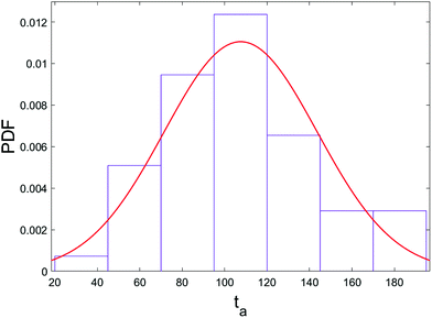
The pressure jump at the x-boundary generates the flow which induces a forced capture and translocation. We adjusted this driving to ensure we are in a regime where the thermal motion and flow force are comparable in the bulk. This can be quantified by the Péclet number that we will define and discuss below. The chain is initially located in the bulk and far from the nanopore and since the motion of the chain is weakly-driven, it is able to diffuse around in the fluid. This is one of the primary differences between our study and most of the previous studies where the chain is placed at the entrance28,37,54–57 and only forced insertion and translocation were investigated. Due to the thermal diffusion, the time required for the chain to reach the converging flow area, the area with significant velocity gradients, may differ between different realizations. As a result, in spite of the drift-controlled regime in the converging area due to the stronger flow, we expect a distribution of centre of mass arrival times ta. Fig. 5 shows a histogram of arrival times of different realizations and the fitted distribution for the 64-mer (we will focus on the 64-mer for explicit calculations in this section). The mean arrival time is 107 ns and the standard deviation of the distribution is wt = 36 ns ± 3 ns. If the chain were a rigid blob moving with the flow, we would expect a single arrival time equal to | (7) |
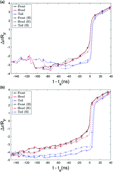
The possibility of unsuccessful capture has been mentioned in literature15,53 and is one of the main reasons that the capture process is considered computationally challenging and as a result has been less studied than translocation. To ensure that the randomness in the arrival time is not stemming from several repeated capture attempts, we monitored the distance of key monomers from the pore entrance as a function of time, as shown in Fig. 6. (The head/tail monomers are the chain ends and the front monomer is the one that arrives at the pore entrance first.) The front monomer initially wanders in the fluid for a reasonable amount of time with an almost constant average velocity. As it approaches the nanopore, the monomer's speed increases and the insertion of the front monomer takes place without any delay (the plot is monotonically increasing as it approaches the pore). As shown in Fig. 6, the velocity of the chain dramatically increases when it arrives at the entrance and the translocation then happens comparably fast.
The extra distance that the chain wanders because of diffusion is denoted as wx and is related to the standard deviation of the probability distribution of the diffusive motion,58
 | (8) |
![[v with combining macron]](https://www.rsc.org/images/entities/i_char_0076_0304.gif) is the average centre of mass speed in the x-direction, D0 is the diffusion constant which we obtained from a separate measurement of mean square displacement versus time. Consequently, the variance of the distance traveled during time ta is wx2 = 2D0ta. Due to the random nature of the diffusion, some particles will need to travel a longer or shorter distance via drift (i.e. movement with the flow). This shorter/longer drift time for distance wx is wt = wx/
is the average centre of mass speed in the x-direction, D0 is the diffusion constant which we obtained from a separate measurement of mean square displacement versus time. Consequently, the variance of the distance traveled during time ta is wx2 = 2D0ta. Due to the random nature of the diffusion, some particles will need to travel a longer or shorter distance via drift (i.e. movement with the flow). This shorter/longer drift time for distance wx is wt = wx/![[v with combining macron]](https://www.rsc.org/images/entities/i_char_0076_0304.gif) where
where ![[v with combining macron]](https://www.rsc.org/images/entities/i_char_0076_0304.gif) is the average centre of mass speed (
is the average centre of mass speed ( , where Δxcom is the initial distance of the centre of mass of the chain from the entrance to the pore). By combining the equations above, we get an estimate for the standard deviation of the arrival time,
 | (9) |
To get a sense of how close to equilibrium the polymer is as its centre of mass (com) moves from its initial position to the pore, we compare the longest relaxation time of the chain tR to a time scale for advection and the mean arrival time. This relaxation time is approximately equal to the time required for the centre-of-mass to diffuse in one direction a distance equal to RF, i.e. tR = RF2/2D0 = 41 ns. We can define two dimensionless numbers related to this. The first, the Péclet number compares the rate of advection to the rate of diffusive relaxation. As the polymer advects in a flow with speed u a distance RF in time tf = Rf/u we can define the Péclet number as
 | (10) |
3.2 Non-equilibrium capture and chain extension
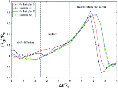
We further investigate the possible deformations of the polymer chain by monitoring the radius of gyration of the chain as a function of the distance of the front monomer from the nanopore (Δr). This is shown in Fig. 7. Both axes are scaled by the equilibrium radius of gyration. As can be seen, far from the nanopore RG fluctuates around the equilibrium value, RG/RF ≈ 1.Although the drag force is comparably weak in the bulk region, it still creates a drift in the x-direction which slowly pushes the chain toward the pore. The drift-diffuse dynamics governs the motion until a part of the chain meets the high intensity flow near the pore. The effect of this flow can be quantified by the Weissenberg number which compares the shear rate to the longest relaxation time of the polymer tR so this can be defined as
| Wi = (shear rate)tR. | (11) |
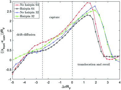
Fig. 8 shows the distance between the front monomer and the centre of mass of the chain as a function of front monomer position. This measure of the chain extension demonstrates that the extension is led by the front monomer being consistently ahead of the centre of mass. The values on both axes are scaled by the equilibrium radius of gyration of the chain. Tracking this distance, one can see the change in the behaviour of this quantity when the front monomer gets closer than rc = 2.5RF to the hole. rc, the capture radius, is the distance from the pore within which the dynamics of the motion alters, the front segment accelerates and the chain begins to extend. The extension of the chain within rc is clearly shown in Fig. 7 and 8. This coincides with the front segment entering the converging flow area where the Wi number is more than one.
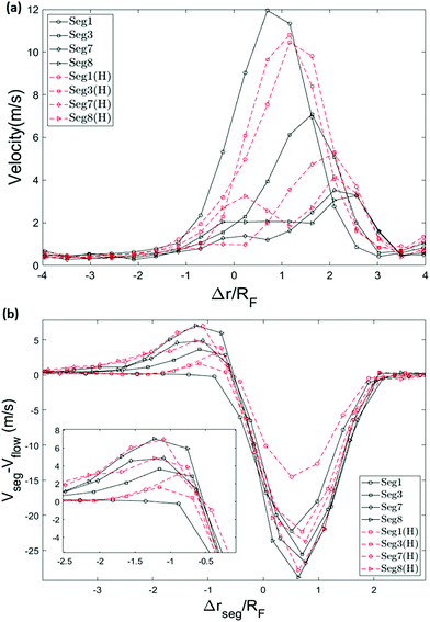
To get a better picture on how the converging flow field affects the dynamics of capture, we take a look at the velocity of the chain. Inspired by the idea behind the blob model,59 the chain is divided into segments and the velocity of different segments are plotted versus the position of the front monomer in Fig. 9a. The segments are numbered from the end that enters the hole first (head) to the end that arrives the last (tail). In both cases, single-file and hairpin capture, the velocity of the segments starts to increase around Δr = 2.5RF in front of the pore. The difference is that for the single-file capture, the acceleration starts from the head and happens sequentially along the chain while for the hairpin capture, the first 3 segments accelerate almost simultaneously and in general, the velocities are more similar.
A similar concept involving a capture radius was introduced for a chain driven by hydrodynamic flow by Daoudi et al.,35 and for electro-osmotic flow by Muthukumar,60 and Grosberg et al.61 Although the possibility of chain extension within the capture radius has been mentioned and mathematically formulated before,35,62 in most of the previous studies on polymer translocation, it was assumed that the whole chain accelerates toward the nanopore within the capture radius and arrives at the entrance as a jammed coil.
In contrast, our simulations shows that the tension created by the converging and accelerating flow deforms the chain as the leading segment enters this area. A mechanism similar to the tension propagation formulated by Sakaue,28 is responsible for the observed deformation which we discuss in the next section. Since the velocity field points toward the hole, the flow guides the front segment to the entrance of the nanopore where the front monomer experiences the maximum force from the flow and gets sucked into the nanopore. This allows for a no-barrier capture in a weakly-driven flow, as shown in Fig. 6. Farahpour et al. obtained similar results in the case of an electric voltage-driven system with the difference that their pore diameter was set so that no hairpin conformation can thread through the nanopore.34 Both acceleration steps can be clearly observed from the radius of gyration graph.
3.3 Tension propagation and effects from the trans-side
The velocity of the translocated monomers falls as soon as they exit the pore on the trans side (this can be seen in Fig. 6). The rate of incoming monomers to the trans side is too fast to allow for relaxation and the chain forms a compacted blob. The drop in the radius of gyration in Fig. 7 is evidence for this contraction. In this section, we discuss the dynamics of the single-file chain during capture and translocation and make a few notes regarding the effect of decompression of the chain on the trans side on the dynamical behaviour of the translocating chain, an interesting effect that is not as well studied.31Fig. 9b shows the speed of segments of the polymer relative to the average fluid flow speed, in the absence of the polymer, as a function of the segment centre-of-mass position. A relative speed of zero in this plot indicates that the segment is moving passively with the fluid flow (i.e. affine motion). Any deviation from zero implies the existence of either tension forces (from other segments) or the presence of backflow. Backflow refers to the influence of the polymer on the flow. This occurs primarily due to the polymer blocking the pore which can slow the fluid flow through the pore. As such, backflow can cause the polymer to move more slowly than the undisturbed flow (i.e. produce negative values in Fig. 9b). However, positive values in the plot (where the polymer is moving faster than the undisturbed flow) can only be caused by tension from neighboring polymer segments pulling the polymer segment. When such a polymer segment moves faster than the undisturbed flow it will also experience a drag force from the fluid resisting this motion.57 The drag force counteracts the tension in the chain segment and results in a decrease in the tension in segments further down the chain.
Far from the pore the whole chain moves with the flow (the pore starts at 0 and extends almost to 1 in Fig. 9). For single-file translocation (black solid lines in Fig. 9b), the first segment (shown with black solid lines with circle markers) is initially moving with the flow (zero relative velocity) until it gets very close to the pore. During translocation, the segment is moving slower than the undisturbed flow field resulting in negative relative velocity. This implies that it is being pulled back by the rest of the chain. Conversely, this means that it is applying an equal and opposite force fc on the rest of the chain which pulls the rest of the chain into the pore. This is evidenced by the positive relative velocities of the non-leading polymer segments as they approach the pore. After leaving the nanopore, the relative velocity of the segment returns to zero.
The tensile force fc propagates along the chain after the insertion of the first segment. When the tension reaches each segment, the velocity of that segment increases beyond that of the surrounding (undisturbed) flow. As mentioned above, this creates a drag force that works against the tension in that segment resulting in a lower tension being passed on to the later segments in the chain. The net result of these effects is a positive peak in the relative velocity observed for segments after the first one. The occurrence of the peak shifts to the left slightly along the x-axis as the tension front reaches rear segments when they are further away from the pore.
Due to the rapid slowing on exiting the nanopore, the translocated segments stay near the exit. As a result, the middle segments traveling through the channel experience an effective repulsion from the dense blob of polymer on the trans side that is in their way. As more monomers are added to this blob, the concentration of monomers rises and the injection of monomers out into the condensed blob becomes more difficult. This condensed blob not just slows the actual speed of the later segments (as seen in Fig. 9a) but also causes the fluid to slow as it also blocks the fluid flow. The deeper valleys in the relative velocity in Fig. 9b for segments further along the chain is evidence of this blocking effect by the condensed blob on both the polymer injection into the blob and the fluid flowing out of the pore.
The story is slightly different for the last segment. Like the middle segments, the relative velocity of the last segment goes through a maximum when the tension front reaches this segment and with drag forces starting to act against its motion the relative velocity decreases. As this segment is last, on exit it is injected into the dense blob on the trans side at its highest density and when the blocking effect on the fluid outflow from the pore is at its maximum. As a result, despite the last segment's motion being free from elastic pullback, it experiences the lowest minimum (most negative) relative velocity of all segments.
The relative velocity of hairpin conformations follows a similar pattern, except for the first segment. The reason for this difference is due to an unraveling mechanism, namely the pulley effect which we discuss in the next section.
3.4 Pulley effect: a single-file capture promoting process
The fact that the part of the chain that reaches the capture distance first is pulled in the flow direction gives a better picture on the formation of hairpins. The hairpin forms when a monomer other than the ends becomes the leading monomer and experiences the stronger force in the converging flow. Fig. 10 illustrates the probability of formation of hairpins at different points along the chain for polymers of length 32 and 64. For a 64-mer, monomers can be indexed from 1 to 64. h is the index of the leading monomer (and the front monomer at the pore entrance) and is therefore the vertex of a hairpin when h > 1. Note that the vertex of the hairpin divides the chain into two strands and that h is also the length of the shorter of these two strands. The x-axis shows the relative location of the vertex of the hairpin along the chain backbone (h = 1 is a single-file conformation). Although the chain enters the nanopore in a single-file form most of the time, a considerable number of entries happen with hairpin conformation. This was also observed in experiments of electrophoretically driven translocation.38 They attributed the high number of entries close to the chain ends to be associated with the entropic freedom of the ends. Because the ends have more freedom compared to other monomers of the backbone, they usually enter the high-velocity region before any other part of the chain and consequently, they are more often dragged into the nanopore as the front monomer.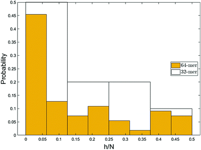 | ||
| Fig. 10 The most probable conformation of insertion is single-file. The probability decreases as the size of the hairpin increases except for very long hairpins (h/N ≥ 0.4). Similar trend was observed in experimental studies.38 Due to chain unravelling and statistical uncertainty, the bin widths of less than 4 monomers would not demonstrate the essential information. | ||
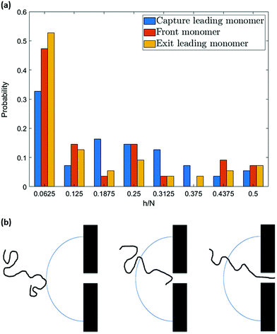
However, the pattern observed in Fig. 10 implies something more. As can be seen, the probability of hairpin insertion decreases as the size of the hairpin increases except for the long hairpins (near 1/2 of chain length) for the 64-mer chain. This result, which was observed in experiments as well,38 suggests that there must be a mechanism by which the medium-size hairpins shift toward long or short hairpins. To explore this matter further, we study the location of the hairpin vertex along the chain as it travels to and through the nanopore. Fig. 11a shows the location in the chain of the leading monomer (the one furthest ahead) at different stages of the process: at the capture radius rc from the pore, at the entrance of the pore (front monomer), and the first monomer to leave the pore (exit). The most striking change is in the first bin of the histogram (i.e. chain end as leading monomer) which increases from 33% at rc to 53% at exit. i.e. the number of realizations with ends as leading monomer increases as the chain moves from the capture radius to the trans side. One can also see that the number of the long hairpins slightly goes up. This graph confirms the existence of the shifting mechanism which we explain by applying a basic force balance argument.
Formation of a hairpin divides the chain into two strands (not necessarily of the same length). The converging flow induces a force on the leading monomer during capture which propagates along the two strands. As discussed in the previous section, this produces a tension in the chain that propagates down both strands, gradually diminishing as it moves away from the leading monomer due to the counteracting drag force of the fluid. If the tension front gets to the end of the shorter strand it is not counteracted by the equal and opposite force from the rest of the chain (of length N − 2h) that is experienced by the corresponding monomer on the longer strand. As a result, the shorter strand accelerates and moves ahead of the longer strand. This is clearly illustrated in Fig. 9b. The relative velocity of the first segment of hairpin conformations is not only positive which indicates that the segment is moving faster than the flow but also exceeds that of segments two and three confirming the unravelling. This causes a deformation which results in the unravelling of the chain (shifting the vertex of the hairpin toward the head of the chain). Due to the resemblance of such a motion to that of a rope on a pulley in a gravitational field, we call this phenomenon the “pulley effect” and illustrate it in Fig. 11b. Depending on the relative position of the chain to the nanopore and the chain conformation, shear-based deformations can facilitate or undo the pulley effect. The strong force in the nanopore dominates the deformation dynamics on the cis side after insertion and the pulley effect is most significantly observed during translocation. As can be seen, the velocity of the first segment of hairpin conformations is significantly higher (i.e. the relative velocity is less negative) than any other segment of hairpin or single-file chains. Although the translocation time is comparably much shorter than the capture time, a reasonable amount of unravelling is observed during translocation, as shown in Fig. 11a (the yellow bar is taller than the orange bar in the first bin) which confirms the discussion above.
If the strands are of equal length (h/N = 0.5) they create comparable forces on the leading monomer and the symmetry of the conformation is preserved during capture and translocation. The tendency toward having a symmetric conformation may be the reason for the shift from h/N ≈ 0.35 to h/N ≥ 0.4. However, due to statistical uncertainty, it is difficult to jump to any further conclusion. The effect of symmetry and tension propagation along symmetric hairpins has also been discussed in a recent theoretical paper by Ghosh et al.63
3.5 The effect of flow strength on capture conformation
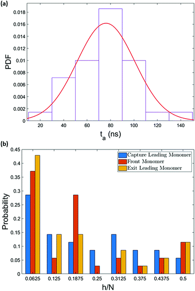
The entropic freedom of the ends and the pulley effect are primarily responsible for the high percentage of single-file captures. Both of these effects depend on the interplay of the driving force and the thermal fluctuations. In our system the flow intensity is controlled by the pressure jump across the box (i.e. at the x-boundary). A higher flow intensity in the bulk results in the chain drifting faster along with the flow and having less time to explore its conformations. The effect of the stronger drift can be observed in the arrival time of the chain. Fig. 12a illustrates the arrival time of the polymer chain for a simulation with 1.4 times higher pressure jump. In addition to smaller mean arrival time compared to the original simulation, the standard deviation of the distribution is also smaller. The narrower distribution is due to the more drift-controlled regime and less time for diffusion.In this case, the ends may be less likely to be the first segments to enter the converging flow. Instead, a hairpin forms from the segment closer to the central axis of the box which has the highest flow intensity. Fig. 12b shows the location of the vertex of hairpins along the polymer's backbone for the system with higher pressure jump. The most probable capture conformation is still single-file, though this peak is smaller than before, and the peak at long hairpins is still present. However, a spike is observed at h/N ≈ 0.2. This is the result of incomplete unravelling. Although the tension propagates along the strands faster with a stronger flow field, the total velocity of the chain also increases which results in shorter arrival and translocation time. Thus, the pulley effect does not get the chance to fully unravel the hairpin. As the chain travels through the nanopore, the pulley effect continues to shorten the hairpin and the spike vanishes for the exiting chain.
4 Conclusion
Polymer translocation as a process entangled with many biological phenomena has attracted researchers' interest from all over science and engineering. Despite all the effort made up to now, the capture process which is a step before translocation has not been well understood which is the motivation behind this work. Using a multiscale simulation package, which takes into account both the hydrodynamic interactions and thermal fluctuations, we observed that a weakly-driven hydrodynamic flow can facilitate the process of finding the pore by the polymer chain and the threading can happen without the requirement of overcoming an entropic barrier.Comparing the arrival time obtained from our simulations and estimated values from mathematical models, we found that the non-uniform and converging flow near the pore speeds up the motion of the chain despite the fact that the motion of the chain is a balanced mix of diffusion and drift in the bulk. By studying the parameters related to the polymer's shape, we discovered that not only does the velocity of the chain increase as a whole but also the stronger flow gradients causes extensions in the polymer.
Moreover, we investigated the possibility of the formation of hairpins and the effect of the extensions on this process. We observed that the single-file insertion is the most probable insertion conformation, as seen in experiments for DNA capture.38 This can be associated with the greater freedom of the ends and the fact that they have a better chance of entering the high velocity area and be guided to the pore. However, the freedom of the ends couldn't explain the quite high number of realizations of single-file and in which long hairpins (almost half of the size of the chain) threaded through the channel. We found out that there is a mechanism, which we call pulley effect, by which the hairpins with strands of considerably different sizes unravel in the favour of shortening the hairpin, but if the strands have comparable length, the chain keeps its conformation and threads through in hairpin shape. The unravelling due to the pulley effect makes single-file capture more probable which means that hydrodynamic flow can be used to promote single-file threading. In particular, one can tune the pressure jump, and hence the fluid flow speed, and potentially other factors such as the shape of the channel and pore itself. These factors could further enhance the pulley effect we observed here.
Conflicts of interest
There are no conflicts to declare.Acknowledgements
This work was supported by the Natural Science and Engineering Council of Canada (NSERC). We would like to thank the Shared Hierarchical Academic Research Computing Network (SHARCNET) and Compute/Calcul Canada for the computational resources.References
- B. Alberts, A. Johnson, J. Lewis, D. Morgan, M. Raff, K. Roberts and P. Walter, Molecular Biology of the Cell: Chapter 9 Visualizing Cells, Garland Pub, USA, 2017, p. 592 Search PubMed.
- M. Muthukumar, Polymer translocation, CRC Press, 2016, pp. 1–342 Search PubMed.
- A. J. Storm, C. Storm, J. Chen, H. Zandbergen, J. F. Joanny and C. Dekker, Nano Lett., 2005, 5, 1193–1197 CrossRef.
- D. W. Deamer, A. Marziali, S. A. Benner, T. Butler, M. Di, C. Link, D. Branton, D. Deamer, A. Marziali, H. Bayley and S. A. Benner, Nat. Biotechnol., 2017, 26, 1146–1153 Search PubMed.
- S. J. Heerema and C. Dekker, Nat. Nanotechnol., 2016, 11, 127–136 CrossRef.
- A. Meller, J. Phys.: Condens. Matter, 2003, 15, R581–R607 CrossRef.
- D. Panja, G. T. Barkema and A. B. Kolomeisky, J. Phys.: Condens. Matter, 2013, 25, 413101 CrossRef.
- V. V. Palyulin, T. Ala-Nissila and R. Metzler, Soft Matter, 2014, 10, 9016–9037 RSC.
- W. Sung and P. J. Park, Phys. Rev. Lett., 1996, 77, 783–786 CrossRef.
- M. Muthukumar, J. Chem. Phys., 1999, 111, 10371–10374 CrossRef.
- J. Chuang, Y. Kantor and M. Kardar, Phys. Rev. E: Stat. Phys., Plasmas, Fluids, Relat. Interdiscip. Top., 2002, 65, 011802 CrossRef.
- J. L. Dubbeldam, A. Milchev, V. G. Rostiashvili and T. A. Vilgis, EPL, 2007, 79, 18002 CrossRef.
- D. Panja, G. T. Barkema and R. C. Ball, J. Phys.: Condens. Matter, 2007, 19, 432202 CrossRef.
- K. Luo, T. Ala-Nissila and S. C. Ying, J. Chem. Phys., 2006, 124, 034714 CrossRef.
- I. Huopaniemi, K. Luo, T. Ala-Nissila and S. C. Ying, J. Chem. Phys., 2006, 125, 124901 CrossRef.
- S. Guillouzic and G. W. Slater, Phys. Lett. A, 2006, 359, 261–264 CrossRef CAS.
- M. G. Gauthier and G. W. Slater, Eur. Phys. J. E: Soft Matter Biol. Phys., 2008, 25, 17–23 CrossRef CAS.
- M. Fyta, J. Sircar, E. Kaxiras, S. Melchionna, M. Bernaschi and S. Succi, Int. J. Multiscale Comput. Eng., 2008, 6, 25–37 CrossRef CAS.
- V. V. Lehtola, R. P. Linna and K. Kaski, Phys. Rev. E: Stat., Nonlinear, Soft Matter Phys., 2010, 81, 031803 CrossRef.
- F. Kapahnke, U. Schmidt, D. W. Heermann and M. Weiss, J. Chem. Phys., 2010, 132, 164904 CrossRef.
- P. Chen, J. Gu, E. Brandin, Y. R. Kim, Q. Wang and D. Branton, Nano Lett., 2004, 4, 2293–2298 CrossRef.
- D. K. Lubensky and D. R. Nelson, Biophys. J., 1999, 77, 1824–1838 CrossRef.
- Y. Kantor and M. Kardar, Phys. Rev. E: Stat., Nonlinear, Soft Matter Phys., 2004, 69, 021806 CrossRef.
- S. S. Chern, A. E. Cárdenas and R. D. Coalson, J. Chem. Phys., 2001, 115, 7772–7782 CrossRef CAS.
- A. Meller and D. Branton, Electrophoresis, 2002, 23, 2583–2591 CrossRef CAS.
- T. Ikonen, A. Bhattacharya, T. Ala-Nissila and W. Sung, Phys. Rev. E: Stat., Nonlinear, Soft Matter Phys., 2012, 85, 051803 CrossRef CAS.
- A. Milchev, J. Phys.: Condens. Matter, 2011, 23, 103101 CrossRef.
- T. Sakaue, Phys. Rev. E: Stat., Nonlinear, Soft Matter Phys., 2007, 76, 021803 CrossRef.
- P. Rowghanian and A. Y. Grosberg, J. Phys. Chem. B, 2011, 115, 14127–14135 CrossRef CAS.
- T. Saito and T. Sakaue, Eur. Phys. J. E: Soft Matter Biol. Phys., 2011, 34, 135 CrossRef.
- T. Saito and T. Sakaue, Phys. Rev. E: Stat., Nonlinear, Soft Matter Phys., 2013, 88, 042606 CrossRef.
- T. Sakaue, Polymers, 2016, 8, 424 CrossRef.
- P. Pincus, Macromolecules, 1976, 9, 386–388 CrossRef CAS.
- F. Farahpour, A. Maleknejad, F. Varnik and M. R. Ejtehadi, Soft Matter, 2013, 9, 2750–2759 RSC.
- S. Daoudi and F. Brochard, Macromolecules, 1978, 11, 751–758 CrossRef CAS.
- T. Sakaue, E. Raphaël, P.-G. de Gennes and F. Brochard-Wyart, EPL, 2005, 72, 83–88 CrossRef CAS.
- A. P. Markesteijn, O. B. Usta, I. Ali, A. C. Balazs and J. M. Yeomans, Soft Matter, 2009, 5, 4575–4579 RSC.
- M. Mihovilovic, N. Hagerty and D. Stein, Phys. Rev. Lett., 2013, 110, 028102 CrossRef.
- N. Ermann, N. Hanikel, V. Wang, K. Chen, N. E. Weckman and U. F. Keyser, J. Chem. Phys., 2018, 149, 163311 CrossRef.
- S. Plimpton, J. Comput. Phys., 1995, 117, 1–19 CrossRef CAS.
- K. Kremer and G. S. Grest, J. Chem. Phys., 1990, 92, 5057–5086 CrossRef CAS.
- S. T. Ollila, C. Denniston, M. Karttunen and T. Ala-Nissila, J. Chem. Phys., 2011, 134, 64902 CrossRef.
- F. E. Mackay, S. T. Ollila and C. Denniston, Comput. Phys. Commun., 2013, 184, 2021–2031 CrossRef CAS.
- S. T. Ollila, C. J. Smith, T. Ala-Nissila and C. Denniston, Multiscale Model. Simul., 2013, 11, 213–243 CrossRef.
- V. Balasubramanian and C. Denniston, Soft Matter, 2018, 14, 9209–9219 RSC.
- S. T. Ollila, C. Denniston, M. Karttunen and T. Ala-Nissila, Phys. Rev. Lett., 2014, 112, 118301 CrossRef.
- S. T. Ollila, C. Denniston, M. Karttunen and T. Ala-Nissila, Soft Matter, 2013, 9, 3478–3487 RSC.
- F. E. Mackay and C. Denniston, J. Comput. Phys., 2013, 237, 289–298 CrossRef.
- B. H. Zimm, J. Chem. Phys., 1956, 24, 269–278 CrossRef CAS.
- M. Doi and S. F. Edwards, The Theory of Polymer Dynamics, Oxford University Press, 1988 Search PubMed.
- W. Humphrey, A. Dalke and K. Schulten, J. Mol. Graphics, 1996, 14, 33–38 CrossRef CAS.
- C. D. Hansen and C. R. Johnson, Visualization Handbook, Elsevier Butterworth-Heinemann, 2005, p. 962 Search PubMed.
- C. Forrey and M. Muthukumar, J. Chem. Phys., 2007, 127, 015102 CrossRef.
- P. Tian and G. D. Smith, J. Chem. Phys., 2003, 119, 11475–11483 CrossRef CAS.
- I. Ali and J. M. Yeomans, J. Chem. Phys., 2005, 123, 234903 CrossRef CAS.
- K. Luo, T. Ala-Nissila, S.-C. Ying and R. Metzler, EPL, 2009, 88, 68006 CrossRef.
- T. Sakaue, Phys. Rev. E: Stat., Nonlinear, Soft Matter Phys., 2010, 81, 041808 CrossRef.
- R. Kubo, M. Toda and N. Hashitsume, Statistical Physics II. Nonequilibrium Statistical Mechanics, Springer Berlin Heidelberg, 1985, vol. 31, p. 279 Search PubMed.
- P. G. de Gennes, Scaling Concepts in Polymer Physics, Cornell University Press, 1979, pp. 1–324 Search PubMed.
- M. Muthukumar, J. Chem. Phys., 2010, 132, 195101 CrossRef CAS.
- A. Y. Grosberg and Y. Rabin, J. Chem. Phys., 2010, 133, 165102 CrossRef.
- C. T. Wong and M. Muthukumar, J. Chem. Phys., 2007, 126, 164903 CrossRef CAS.
- B. Ghosh, J. Sarabadani, S. Chaudhury and T. Ala-Nissila, Pulling a folded polymer through a nanopore, 2019, http://arxiv.org/abs/1912.07974.
| This journal is © The Royal Society of Chemistry 2020 |

