
Diffuso-kinetic membrane budding dynamics†
Rossana
Rojas Molina
a,
Susanne
Liese
 a,
Haleh
Alimohamadi
b,
Padmini
Rangamani
b and
Andreas
Carlson
*a
a,
Haleh
Alimohamadi
b,
Padmini
Rangamani
b and
Andreas
Carlson
*a
aMechanics Division, Department of Mathematics, University of Oslo, 0316 Oslo, Norway. E-mail: acarlson@math.uio.no
bDepartment of Mechanical and Aerospace Engineering, University of California, San Diego, CA 92093, USA
First published on 14th October 2020
Abstract
A wide range of proteins are known to create shape transformations of biological membranes, where the remodelling is a coupling between the energetic costs from deforming the membrane, the recruitment of proteins that induce a local spontaneous curvature C0 and the diffusion of proteins along the membrane. We propose a minimal mathematical model that accounts for these processes to describe the diffuso-kinetic dynamics of membrane budding processes. By deploying numerical simulations we map out the membrane shapes, the time for vesicle formation and the vesicle size as a function of the dimensionless kinetic recruitment parameter K1 and the proteins sensitivity to mean curvature. We derive a time for scission that follows a power law ∼K1−2/3, a consequence of the interplay between the spreading of proteins by diffusion and the kinetic-limited increase of the protein density on the membrane. We also find a scaling law for the vesicle size ∼1/(![[small sigma, Greek, macron]](https://www.rsc.org/images/entities/i_char_e0d2.gif) avC0), with av the average protein density in the vesicle, which is confirmed in the numerical simulations. Rescaling all the membrane profiles at the time of vesicle formation highlights that the membrane adopts a self-similar shape.
avC0), with av the average protein density in the vesicle, which is confirmed in the numerical simulations. Rescaling all the membrane profiles at the time of vesicle formation highlights that the membrane adopts a self-similar shape.
1 Introduction
In a wide range of cellular processes, membrane shape remodeling due to the association and dissociation of proteins plays a fundamental role, e.g., endo- and exocytosis,1 virus assembly2 and the formation of intracellular compartments.3 The presence of proteins on the membrane leads to changes in biomechanical properties such as bending rigidity,4 diffusion coefficient of proteins5,6 and membrane curvature. The molecular machinery associated with curvature-inducing processes is often complex7,8 and while some involve active motor proteins,9–11 there is a multitude of proteins that are able to passively induce membrane shape transformations.8,12 The biophysical mechanisms that induce membrane curvature include the insertion of amphipathic helixes into the bilayer,13 producing an area difference between the inner and outer membrane leaflet through the binding of large proteins to one membrane side14,15 or protein crowding.16,17 Thus, the net effect of any asymmetry between the leaflets of the bilayer due to anchoring inclusions or steric pressure can be represented by the spontaneous curvature.18Reconstituted and synthetic vesicles are essential model systems that help to reveal the fundamental biophysical mechanisms by which proteins are able to induce membrane shape transformations.16–21 For instance, experiments have demonstrated that the formation of tubular structures is directly correlated with the protein density on the membrane16 and that protein crowding correlates with the formation and abscission of vesicles.17 Moreover, it has been shown experimentally that the local membrane curvature and the resulting membrane shape is coupled to the concentration of curvature-inducing macromolecules. For example, tubular structures that are formed by anchoring polymers, shrink as diffusion reduces the local polymer density.21
A typical membrane remodeling process starts from a flat surface and develops into a deformed membrane with the shape of a bud, vesicle or tubule22,23 as proteins are locally recruited to the membrane surface and induce a spontaneous curvature.24,25 Membrane deformation is thus driven by a gradual recruitment and accumulation of membrane-associated proteins and changes in physical properties over time,8 suggesting that in order to derive a theoretical description of the dynamic evolution of a membrane shape we must include the recruitment of curvature-inducing proteins.
Over the years, numerous theoretical studies have been dedicated to describe a wide range of mechanisms that play a vital role in various cellular processes, i.e. diffusion of transmembrane proteins,26 protein crowding27–29 and spontaneous curvature induced by macromolecules such as polymers and proteins.18,21,30–32 More complex theoretical models also include the viscous dissipation generated as the proteins move on the lipid bilayer,33,34 as well as non-local hydrodynamics where the entire flow field is resolved.35–37
Since the thickness of a lipid bilayer is much smaller than the typical length scale of membrane deformations, it is common to treat biomembranes as elastic thin sheets.38–41 Similarly, the size of an individual protein is at least an order of magnitude smaller than the extension of a membrane bud or vesicle, which justifies to describe the proteins as a continuous field. Previous theoretical studies have investigated various aspects of membrane deformation generated by concentration-dependent spontaneous curvature, considering either a static protein distribution on the membrane42–45 or including diffusion dynamics.26,30,34 In addition, a theoretical framework based on the Onsager variational principles has been developed, where the dynamics are given by the balance between dissipative and driving forces.33,46,47 This framework gives a compact mathematical description of adsorption and desorption of proteins from the bulk and its diffusive dynamic on a fixed membrane shape.
Compared to the diffusive protein dynamics on membranes, far less is known about the dynamic interplay between diffusion, local protein kinetics and membrane shape changes, where a theoretical model considering all three processes has not yet been explicitly established. In this study, we develop such a model with a focus on finding temporal relationships between the kinetics of protein recruitment and the timescales of bud formation.
To study the spatio-temporal budding process of a membrane, we develop a minimal mathematical model for the diffuso-kinetics of membrane associated proteins. We treat the concentration of proteins as a continuous field following a diffusion equation with an adsorption term, describing the protein recruitment from a reservoir i.e. the cytosol or the extracellular space, and a detachment term representing the protein turnover. Additionally, our model incorporates that the protein concentration induces an effective local spontaneous curvature on the membrane, which drives the membrane shape evolution. Finally, to characterize the membrane deformation dynamics we span the phase space by varying the kinetic parameters and the protein sensitivity for the detection of membrane curvature to uncover scaling relationships between time for scission and kinetic recruitment parameters of proteins onto the membrane.
2 Theoretical model
2.1 Energy functional
To study how proteins that are bound to biological membranes influence the membrane shape evolution, we begin by defining the membrane energy per unit area W, which includes the bending energy, surface tension and entropic effects due to membrane–protein interactions given by:41,46,48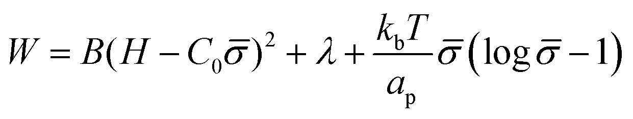 | (1) |
The first term is the Helfrich energy,26,38 where H is the mean curvature and B is the bending rigidity. The Helfrich model is suitable to describe cases where the radii of membrane curvatures are much larger than the thickness of the bilayer,40 allowing us to treat the lipid bilayer as a thin elastic shell. Here, we assume that the induced spontaneous curvature C = C0 due to membrane–protein interactions depends linearly on the protein density,26,48,49 where C0 is a proportionality constant associated to the spontaneous curvature induced by one protein and is the protein density on the membrane scaled by the saturation density.49 The proteins are mobile on the membrane, hence the density varies in time and space.
The second term in eqn (1) is the surface tension. We describe the membrane as an infinite surface, where the far-field acts as a lipid reservoir. In this case, a constant surface tension λ acts along the entire membrane. The third term accounts for entropic effects. When the protein density in the membrane surface is small and the available binding sites for the proteins are not bounded, the entropy term is well approximated by the mixing entropy of an ideal gas.46,50,51 This model is simpler than the general Langmuir absorption model,52,53 where kb is the Boltzmann constant, T is the temperature and ap is the area occupied by one protein.
Additional terms may be included in W (eqn (1)), such as interaction terms between proteins ∼2 and the energy cost arising from density gradients ∼(∇).2,48,54 Both terms scale with the magnitude of the protein–protein interaction. Since the non-specific interaction between proteins is weak compared to the bending and entropic energy, the interaction and gradient terms can be neglected. In the ESI,† (Section S8), we estimate the contribution to the energy functional by the interaction between proteins and the density gradients, to illustrate that the mixing entropy is the leading contribution to the energy, thus simplifying its description. To keep the mathematical model minimal, we assume that both the Gaussian bending modulus and the bending rigidity B are constant, i.e., they do not depend on the local protein density, which also implies that the Gaussian bending energy is a constant, since we do not consider topological changes such as membrane scission.30,55
2.2 Membrane shape equations
The axially symmetric membrane is described in the arc-length parametrization with the radial and vertical components r = r(s) and z = z(s) and the tangent angle ϕ = ϕ(s), where s is the arc-length. A schematic representation of the system and the coordinates are shown in Fig. 1.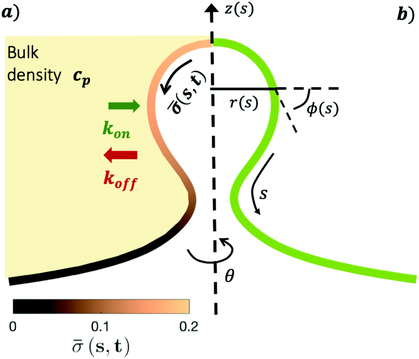 | ||
| Fig. 1 (a) The proteins in the bulk have a constant volume density cp, represented by a uniform light yellow color. The proteins attach to the membrane at a rate kon and detach from it at a rate koff. The attached proteins on the membrane can diffuse on the surface of the membrane and also induce a spontaneous curvature proportional to the protein concentration (s,t) represented as a color gradient, which evolves in time according to a diffusion process coupled with kinetic recruitment and detachment leading to an inhomogeneous protein distribution on the membrane. (b) A description of the membrane surface parametrization in axisymmetric coordinates. Here s is the arc-length measured along the membrane, r(s) is the radial coordinate, ϕ(s) is the angle that the curved membrane forms with respect to the horizontal r-axis and z is the height of the membrane. The angle θ is the rotation around the symmetry axis. | ||
The mean curvature H in the arc-length parametrization is given by:56
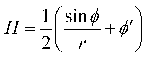 | (2) |
The operator 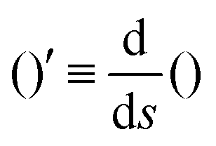 represents the derivative with respect to the arc-length s.
The arc-length parametrization allows to express the coordinates r, z and the area of the membrane, A, in the following way:
r′ = cos![[thin space (1/6-em)]](https://www.rsc.org/images/entities/char_2009.gif) ϕ ϕ | (3) |
| z′ = sinϕ | (4) |
| A′ = 2πr | (5) |
The shape of the membrane for a given protein distribution is such that it must minimize the total energy, given by the integral of eqn (1) over the total area of the membrane, 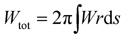 .
.
To derive the energy minimizing shape, we define ![[script L]](https://www.rsc.org/images/entities/char_e144.gif)
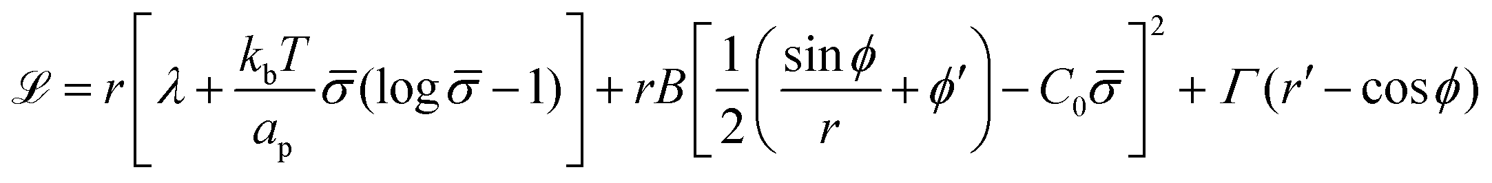 | (6) |
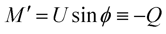
The bending moment of the membrane, M, is given by:58
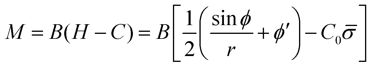 | (7) |
From eqn (7) we obtain the differential equation for the angle ϕ as:
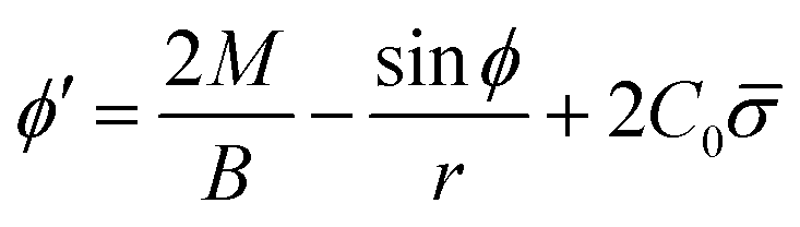 | (8) |
Finally, following the Euler–Lagrange formalism, we obtain (see the ESI,† for details):
 | (9) |
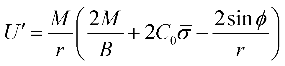 | (10) |
The boundary conditions implemented to solve the set of 6 equations given by eqn (3)–(5) and (8)–(10), which enforce a transition into a flat membrane at the outer boundary, are described in detail in the ESI.†
2.3 Spatio-temporal dynamics of the protein concentration
At cell membranes proteins are recruited and disassociated in kinetic binding and unbinding processes7,8,59 while they diffuse along the membrane.5,6 Hence, the dynamics of the protein density(s,t) is described by a diffuso-kinetic equation with two contributions: the diffusive part, ![[scr E, script letter E]](https://www.rsc.org/images/entities/char_e140.gif) diff, and the recruitment/turnover part, source. The two terms have to fulfill diff = source, implying that the flux of proteins along the membrane arises from a protein source/sink. The general form of diff is written as:
diff, and the recruitment/turnover part, source. The two terms have to fulfill diff = source, implying that the flux of proteins along the membrane arises from a protein source/sink. The general form of diff is written as: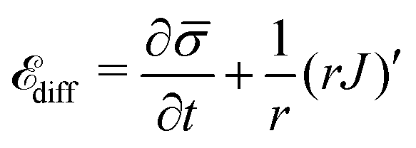 | (11) |
and the second term is the surface divergence of the protein flux J in axially symmetric coordinates.
In general, the protein flux is given in terms of the chemical potential derived from the energy functional in eqn (1), 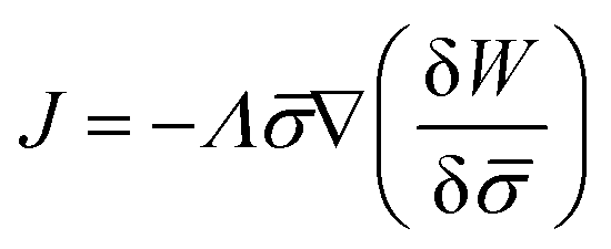 .46,60Λ is the protein mobility and
  is the functional derivative of the energy functional W with respect to the protein density. In the absence of gradient terms in the energy, the functional derivative reduces to
  .61 Hence, the non-vanishing component of the flux, J, is given by:
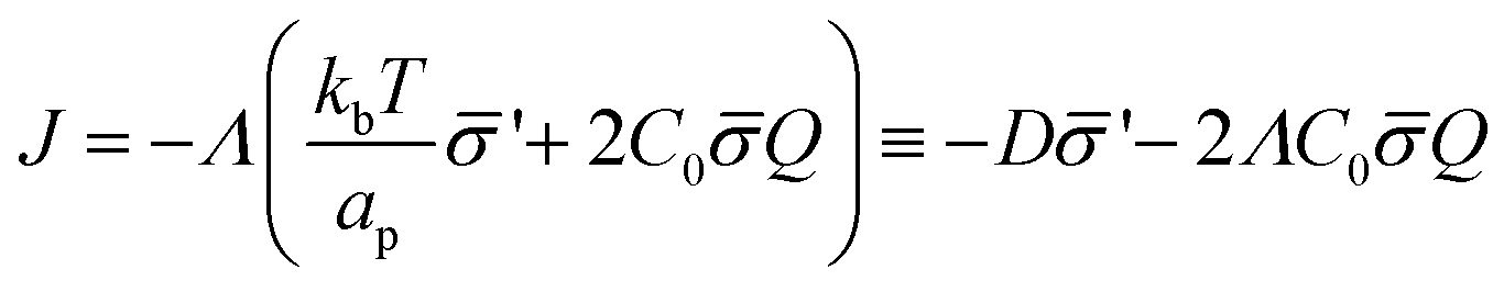 | (12) |
 is the diffusion coefficient and Q is defined in eqn (9). Eqn (12) recovers a diffusive flux on a flat surface, in the limit, C0 ≈ 0, which implies that the membrane is flat in this limit, as the proteins have no influence in the membrane shape. However, in the general case the flux has a non-negligible contribution arising from the curvature of the membrane, via the function Q. Finally, the explicit form of diff is:
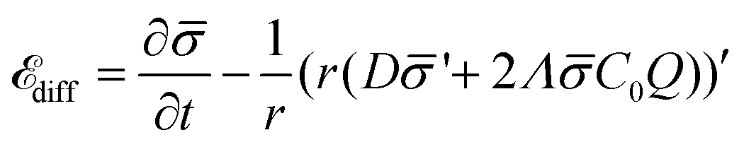 | (13) |
To model the protein recruitment, we make four assumptions: first, the recruitment is modeled following the linear adsorption–diffusion model,46 in which it is assumed that the protein density is small, and that the available binding sites for the proteins are not bounded, as in the more general Langmuir absorption model. Second, we assume that the protein density in the bulk is constant. Third, protein recruitment is triggered when the membrane curvature exceeds a threshold value H0. This assumption is inspired by experimental observations, which found that certain proteins are enriched in curved regions of the membrane62,63 with the ability to also induce a curvature.64 Theoretical studies based on molecular dynamics simulations65 and Monte Carlo simulations66 have shown that various biophysical mechanisms can cause curvature sensing, where proteins adsorb to a membrane in a step-like manner with respect to the membrane curvature. We incorporate these key characteristics in a phenomenological curvature sensing model by multiplying the on-rate by a Heaviside function Θ(H − H0) and show in the ESI† (Section S7) that regularizing the Heaviside function does not affect the prediction as long as the jump is sufficiently steep. Lastly, we consider the diffuso-kinetic dynamics i.e. out equilibrium, which is further illustrated below by our numerical simulations. We acknowledge that a more complex relation between the recruitment kinetics and the membrane curvature might be proposed,67 which requires a more elaborated theoretical treatment also satisfying detailed balance at equilibrium. To the best of our knowledge, a universal model for curvature-sensitive recruitment dynamics is still a topical question in the field.
In light of these assumptions, the mathematical form of source can be written as:
| source = cpkonΘ(H − H0) − koff | (14) |
| Parameter | Typical value |
|---|---|
| Membrane thickness h | 5 nm68 |
| Membrane viscosity ηm | (10−9–10−7) N s m−133,69,70 |
| Cytosol viscosity ηc | (1–4) × 10−2 N s m−271,72 |
| Spontaneous curvature of one protein C0 | (0.075–0.2) nm−173,74 |
| Area of one protein ap | (16–70) nm217,19,74 |
| Bulk concentration of proteins cp | (0.1–50) μM17,59 |
| Dissociation constant KD | (0.1–5) μM59 |
| Diffusion coefficient D | (0.01–1) μm2 s−175,76 |
| Bending rigidity B | (20–40)kBT43,74 |
| Surface tension λ | (0.003–0.3) × 10−3 N m−174,77 |
To understand which process sets the time scale of the membrane dynamics, we perform a scaling analysis. The rate of change of the bending energy can be dissipated by membrane viscosity, i.e., 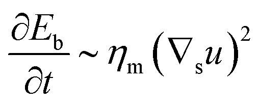 , where Eb = B(H − C0)2 is the bending energy, ηm is the membrane viscosity and u is the membrane velocity. The bending energy scales as Eb ∼ B/L2, u ∼ L/τv, where τv is the viscous time scale and ∇ ∼ 1/L, giving B/τv ∼ ηmL2/τv2. We can then write τv ∼ ηmL2/B. On the other hand, the diffusive time scale is given by τD ∼ L2/D, where the diffusion coefficient D is related to the membrane viscosity ηm through the Saffman–Delbruck theory,78 where
 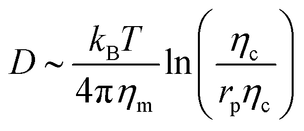 . Here, ηc is the viscosity of the cytosol and rp ∼ 5 nm is the typical radius of one protein. With the typical values of the membrane and cytosol viscosity in Table 1, the diffusion coefficient
 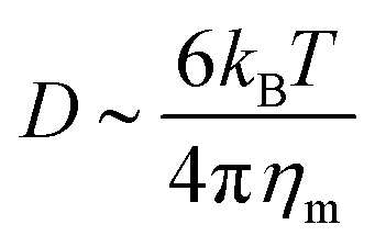 . The ratio between these two time scales becomes
 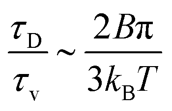 . With B ∼ 20kBT, we obtain that
 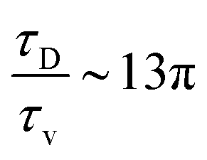 , that is, the diffusive time scale can be more than one order of magnitude larger than the viscous time scale, supporting our assumption that the mechanical relaxation of the membrane is fast compared to its diffusive transport of proteins.
The equation governing the time evolution of , diff = source in non-dimensional form is written as (see the ESI† for details):
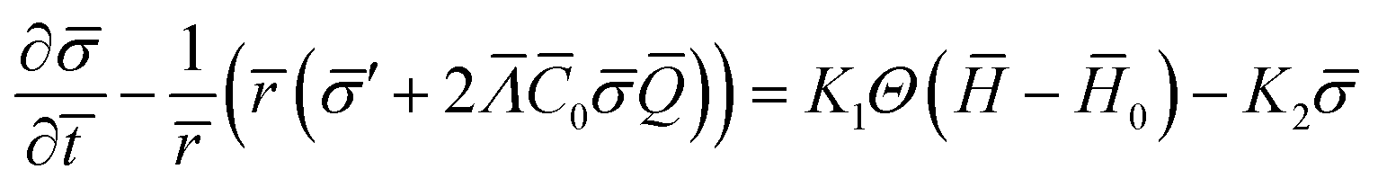 | (15) |
eq), i.e., the length scale given by the spontaneous curvature C0 induced by the recruited proteins and the equilibrium density of proteins, eq = K1/K2, obtained as all gradients vanish in eqn (15). Time has been scaled with τD. The energy has been scaled with the bending rigidity B. Introducing the scaling into the governing equations gives us the scaled variables, 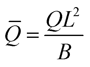 ,
,  ,
,  ,
, ![[H with combining macron]](https://www.rsc.org/images/entities/i_char_0048_0304.gif) = HL,
= HL,  and the dimensionless numbers,
  ,
, ![[C with combining macron]](https://www.rsc.org/images/entities/i_char_0043_0304.gif) 0 = C0L and 0 = H0L, K1 = cpkonL2/D, K2 = koffL2/D. To ease the notation, we drop all the bars from eqn (15) and for simplicity we keep
0 = C0L and 0 = H0L, K1 = cpkonL2/D, K2 = koffL2/D. To ease the notation, we drop all the bars from eqn (15) and for simplicity we keep  .
.
The non-dimensional number K1 = cpkonL2/D is the ratio between the diffusive time scale and the kinetic recruitment time scale and K2 = koffL2/D is the ratio between the diffusive time scale and the protein turnover time scale. 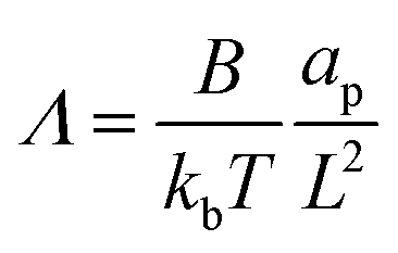 is the ratio of the bending energy and the thermal energy. In addition, we set the surface tension λ to be zero, but the influence of λ > 0 is further discussed in the ESI.† The ratio between K1 and K2 can be written in terms of the dissociation constant KD as
 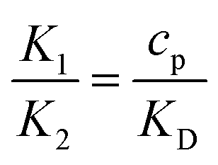 . Since we assume the protein density is small as compared to the saturation density, K1 and K2 must be chosen in such a way that the equilibrium density of proteins in the membrane is small. To reduce the number of parameters influencing the dynamics we set K1/K2 = 1/5 in all the numerical simulations, which for t = ′ = 0 = K1 − K2 gives = 1/5 < 1, consistent with a system where the recruitment is slower that the turnover of proteins. We have chosen B = 20kBT, C0 = 0.1 nm−1, and ap = 27 nm2, which gives C0 = 5 and Λ = 0.22 in eqn (15) and point out that eqn (8) and (10) are the only shape equations that have a non-dimensional parameter in them, which is C0. The rest of the shape equations, eqn (3)–(5) and (9) are parameter-free. The non-dimensional numbers K1 and H0 form the basis of a parameter space that will allow us to determine the dependence of the membrane shape with respect to the coupling between diffusion and kinetics.
As we span the phase space of H0 ∈ [0.0015–0.15] and K1 ∈ [0.2–9] we observe formation of thin membrane necks with respect to the rotational axis r = 0. Since the mathematical model is no longer valid if the neck width is comparable in size with the membrane thickness, we consider the numerical results up to the point when the neck width is equal to the membrane thickness h, that in non-dimensional form has the value h = 0.1 and corresponds to the membrane thickness h reported on Table 1. We define the scission time as tcut. The range of H0 corresponds to a radius of curvature of about 300 nm to 30 μm, covering the typical size range of cells (≈6 μm), membrane-bound vesicles (≈500 nm) and giant unilaminar vesicles (up to 200 μm).22,79
3 Results
We begin by illustrating the dynamic formation of two characteristic membrane shapes obtained using numerical simulations based on eqn (3)–(5) and (8)–(10) and eqn (15) for H0 = 0.0015 (Fig. 2) and H0 = 0.15 (Fig. 3). Initially the membrane is flat with a small initial protein density near the axis of symmetry r = 0, which we model as a Gaussian profile with small amplitude and width(s,t = 0) = 0.1e−(s/0.3)2. The initial amplitude of the protein density on the membrane plays a minor role in the budding dynamics, as the scission time tcut is insensitive to the initial amplitude of the Gaussian profile (see ESI,† Section S6). This initial protein density induces a change in the spontaneous curvature and generates a small membrane deformation. The proteins start to be recruited and redistributed on the membrane, inducing a deformation that goes through a set of different shapes: bump (Fig. 2a and 3a), U-shape (Fig. 2b and 3b), Ω-shape (Fig. 2c and 3c) and at the final stage a pearl, when H0 = 0.0015 (Fig. 2d) or a single bud, when H0 = 0.15 (Fig. 3d). These structures are also found for non-vanishing, but small surface tension, as shown in the ESI† (Section S9). From Fig. 2 and 3 we see that the parameter H0, i.e. the proteins sensitivity to mean curvature, plays an important role in determining the final shapes of the membrane. If H0 is small, pearled structures can be observed, whereas if H0 is larger (H0 ≫ 0.0015), the formation of smaller, single buds is favored. A low value of H0 (H0 = 0.0015) leads to recruitment to a large area of the membrane and it adopts a pearl-like structure. In contrast, when H0 is larger (H0 = 0.15), an almost spherically shaped membrane emerges from the initially flat membrane, caused by the recruitment of proteins to a smaller area of the membrane, as compared to a smaller H0. There are also some other noteworthy features we would like to highlight: Despite the fact that K1 is identical for the two simulations, the proteins are distributed over a different area. Besides the obvious differences in shape, it appears that also H0 will determine the continuation of the process for t > tcut. If a vesicle is shed from the membrane at t = tcut in Fig. 2d the rest of the membrane will still have a significant portion covered by curvature inducing proteins and it appears that another vesicle will form from the Ω shape. When H0 is larger a single vesicle forms (Fig. 3d), which contain almost all the proteins. In this case, after scission the membrane may return to its undeformed state stalling the dynamics.
 | ||
| Fig. 2 Characteristic membrane shapes at four different snapshots in time when the dimensionless rate coefficient is K1 = 4.5 and the threshold for protein recruitment is H0 = 0.0015. As we march forward in time the membrane deforms from a nearly flat membrane (not shown) into a pit-shape (a), an U-shape (b), an Ω-shape (c) and finally into a pearl-like membrane shape (d). The color bar represents the protein density (s,t). In (c) and (d) the protein density is almost uniform on the vesicle at the top of the budding structure and decays gradually along the rest of the deformed membrane. The scale bar is the dimensionless unit length of the system, equivalent to L = 50 nm. | ||
 | ||
| Fig. 3 Characteristic membrane shapes at four different snapshots in time when the dimensionless rate coefficient is K1 = 4.5 and the threshold for protein recruitment is H0 = 0.15. Similarly to the intermediate shapes shown in Fig. 2a–c, we observe that here the membrane shape exhibits a pit-shape (a), U-shape (b) and Ω-shape (c), but at t = tcut a single bud with a constricted neck is formed (d) instead of a pearl, as in Fig. 2d. The color bar represents the protein density (s,t). In (c) and (d) we also observe and almost constant protein density on the vesicle, but it rapidly decays outside of the neck. The scale bar is the dimensionless unit length of the system, equivalent to L = 50 nm. | ||
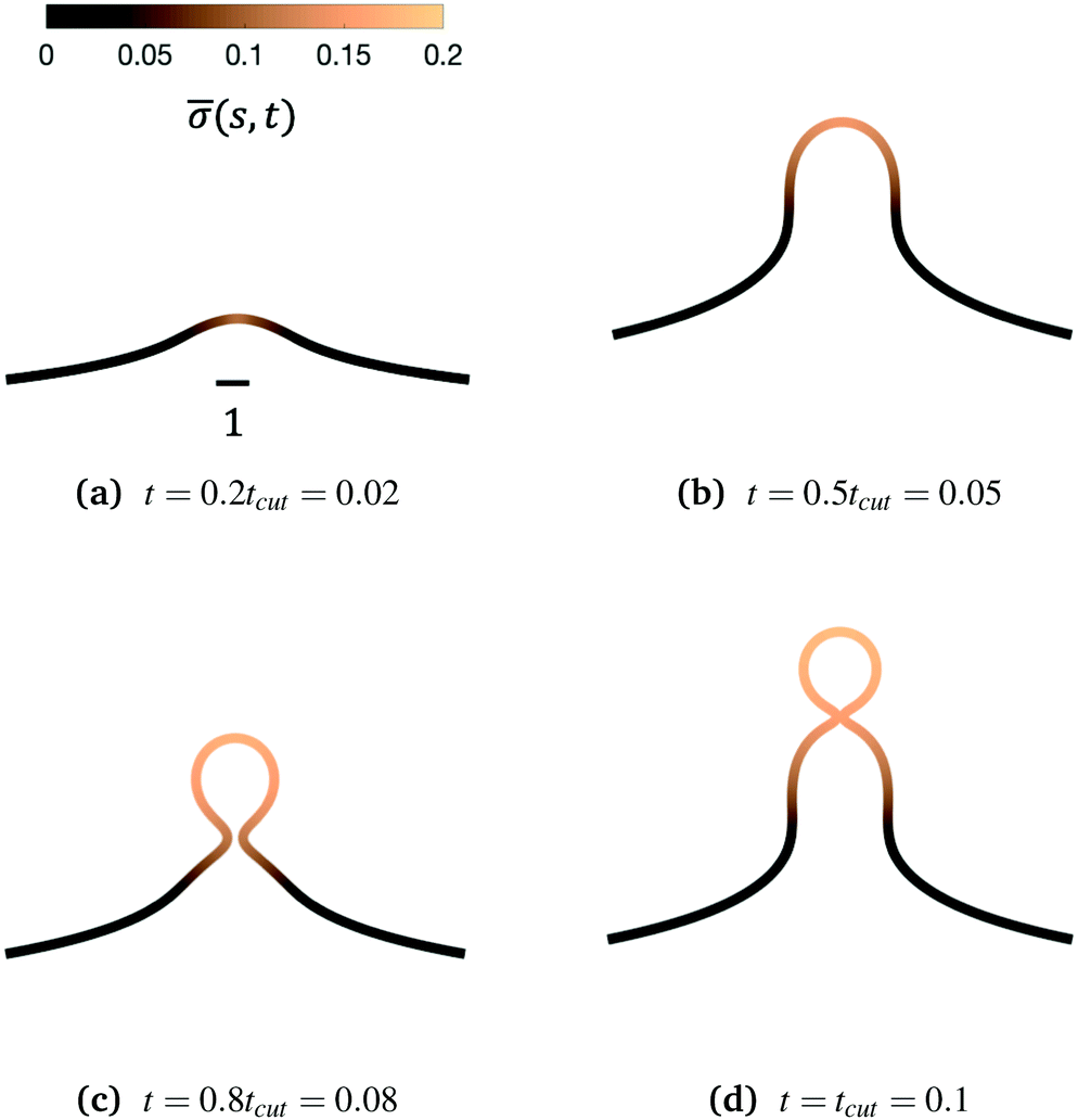
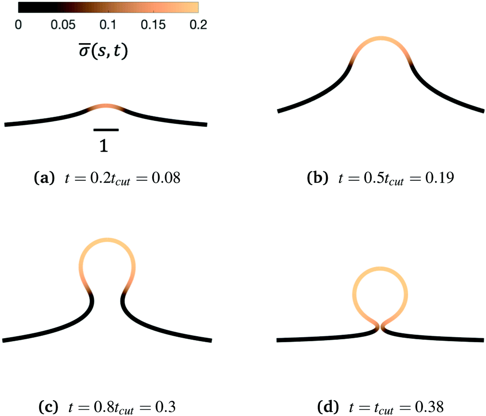
To see the details of the protein distribution on the membrane in Fig. 2 and 3, we plot in Fig. 4 the protein density as a function of the membrane area A. In order to clearly illustrate the influence of H0 on the protein distribution over the membrane we extract at the same snapshots in time as in Fig. 2 and 3 using the time for membrane scission tcut as a point of reference: t = 0.2tcut, 0.5tcut, 0.8tcut and tcut where [H0 = 0.0015, tcut = 0.1] and [H0 = 0.15, tcut = 0.38]. A general feature is that the protein density is distributed over a larger area on the membrane when H0 is small and it has a smaller gradient as we move from the axis of symmetry to the undeformed membrane. In contrast, when H0 is larger the proteins are limited to a much smaller region of the membrane with a steep decay in . By inspecting Fig. 4a–d we can notice the growth rate of the area covered by proteins is much faster when H0 is small. To see this, we can roughly estimate the rate of change of covered area ΔA in the time interval Δt = (0.5 − 0.2)tcut, which for H0 = 0.0015 is ΔA/Δt ∼ 600 contrasting the same calculation ΔA/Δt ∼ 50 when H0 = 0.15. During the last stages of the membrane deformation (Fig. 4b–d) the area covered by proteins increases much slower once an Ω-shape is formed (see Fig. 2b–d and 3b–d) and at the last stage (Fig. 4c and d) this area barely increases and just an increment on the protein density is observed on the membrane for both values of H0. Thus, the geometry of the membrane may also play a role in the dynamic growth process. H0 appears to be a critical parameter, because it determines not only the overall size of the budding structures, but also determines in part how proteins are distributed on the membrane. Fig. 4d also shows that as a single vesicle forms (H0 = 0.15) the recruited proteins leave the membrane and stalls the dynamics, contrary to when proteins are almost insensitive to the mean curvature and covers a much larger membrane area (H0 = 0.0015).
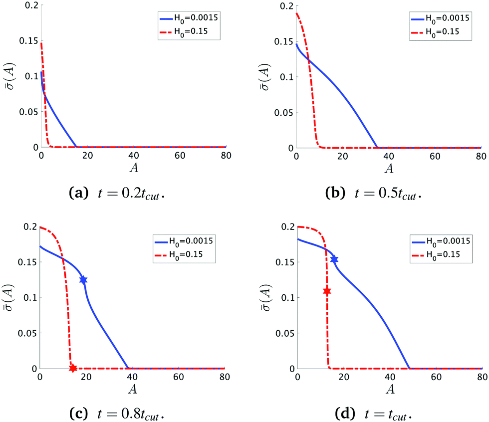 | ||
| Fig. 4 Characteristic protein density at four different snapshots in time when the dimensionless rate coefficient is K1 = 4.5 and the threshold for protein recruitment is H0 = 0.0015 and H0 = 0.15. At first ((a) and (b)) (A,t) decays nearly linearly with A from the maximum at the symmetry axis r = 0, but once an Ω-shape is formed (c) (A,t) in the vesicle is more uniform whereas the steepest decay in occurs from the membrane neck to the undeformed membrane, specially when H0 = 0.15. In (c) we observe that there are proteins distributed in the region beyond the vesicle neck when H0 = 0.0015 but there are no protein outside the vesicle when H0 = 0.15. (d) At t = tcut we observe that the protein density in the membrane neck does not vanish. The star shaped markers in (c) and (d) represent the position of the neck (smallest radius at that given point in time). | ||
To further characterize qualitatively the membrane dynamics we extract the height of the membrane, zmax, along the symmetry axis r = 0 for K1 = 4.5 when H0 = 0.0015 (Fig. 5a) and H0 = 0.15 (Fig. 5b). Initially, we can observe that zmax increases as the membrane bud grows in size, but as the membrane starts to form an Ω-shape its height starts to decrease as the neck constricts. The features of zmax also allows us to identify the pit-, U- and Ω-shape of the membrane already shown in Fig. 2 and 3. When the membrane forms a pearl-like shape, the bud growth and neck constriction happens several times. The insets in Fig. 5a show the shapes corresponding to the first maximum and the first minimum of zmax as well as the final shape at t = tcut. In the time interval between the first maximum and first minimum in zmax(t), the membrane shows a gradual transition between a pit-, U- and Ω-shape. As the neck size in the Ω-shape corresponding to the first minimum of zmax in Fig. 5a is larger than the typical width h of the membrane bilayer, its height starts to increase again forming a vesicle at the top of the newly formed Ω-shape as we march forward in time. The oscillatory behaviour of zmax is not observed when H0 = 0.15 (Fig. 5b) but zmax has a similar growth and decay when the Ω-shaped membrane is formed.
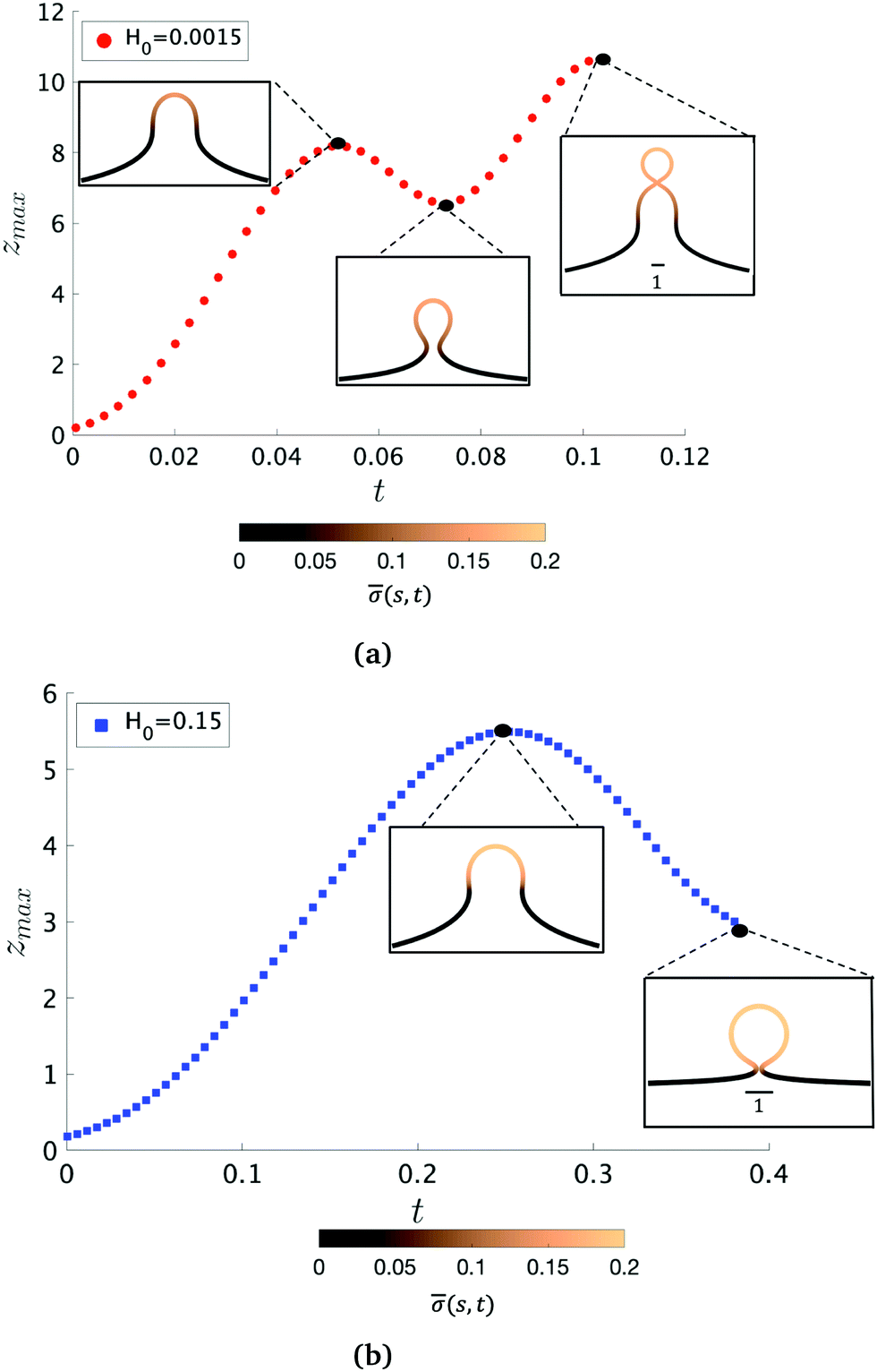 | ||
| Fig. 5 The maximum height of the membrane with respect to its symmetry axis, zmax, as a function of time, for K1 = 4.5 and for different values of H0. In (a) it is shown that zmax oscillates. Once a pit shape is formed and zmax starts to decrease (first maximum of zmax), an Ω-shape starts to emerge. During the decrease of zmax, up to the first minimum of zmax in (a) the construction of the bud neck proceeds. As at this stage the neck radius is larger than the membrane thickness, the membrane shape evolution leads to a pearl structure at a later time (t = tcut). In contrast, a higher value of H0 prevents oscillation on zmax, as shown in (b). The color bar represents the protein density along as a function of the arc-length s and time t, (s,t). | ||
Next, we turn to map out the membrane shapes predicted by the mathematical model at the scission time, i.e. t = tcut, by systematically varying K1 ∈ [0.2–9] and H0 ∈ [0.0015–0.15], see Fig. 6. As we go through the parameter space we see how the values of the non-dimensional numbers K1 and H0 determine if a vesicle buds directly from the membrane or on a deformed foundation as a pit, U or Ω-shape. The phase space in membrane shapes also suggests that we can distinguish membrane deformations that are likely to form only a single vesicle (H0 = 0.15) and those that appear to continuously form vesicles by budding from a pit-shape (H0 = 0.015, K1 = 1.4, 4.5, 9 and H0 = 0.0015, K1 = 9), U-shape (H0 = 0.0015, K1 = 4.5) and Ω-shape (H0 = 0.0015, K1 = 1.4). Qualitatively we can understand the effect of H0 by associating this parameter with the membrane region where recruitment of protein occurs: The inverse of H0 sets a length scale that becomes large for small H0, then proteins are recruited into a larger portion of the membrane, leading to larger budding structures such as pearls (see Fig. 6), while for larger H0 this length scale will become smaller and in this case smaller budding structures would be expected.
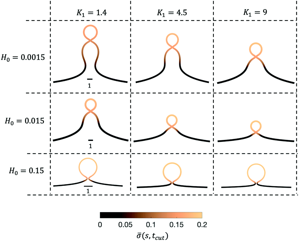 | ||
| Fig. 6 The membrane shapes at t = tcut for K1 ∈ [0.2–9] and H0 ∈ [0.0015–0.15]. The color bar represents the protein concentration as function of the arc-length at t = tcut, (s,tcut). Note that the scale bar is not the same for the different values of H0. | ||
The exploration of the phase space spanned by the parameters K1 and H0 also allows us to determine how they affect the dynamics of the membrane deformation. One quantity that helps to illustrate the time scale of the budding process is tcut. The scission time is measured as the neck size reaches h = 0.1 in the radial direction, see Fig. 7a. In Fig. 7b we present the dependence of tcut with respect to K1 in logarithmic axis. Interestingly, we find a universal behaviour: tcut ∼ K1−2/3 despite that we vary K1 over two orders of magnitude and changing H0 only affects the pre-factor of the scaling relation and not the power law. The universal behaviour suggests that the same mechanisms are present across different simulations, where there is a complex interplay between the membrane geometry, diffusion and the area limited for protein recruitment.
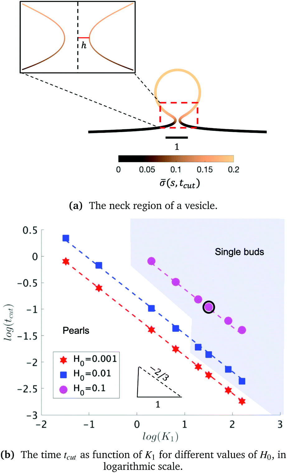 | ||
| Fig. 7 (a) The membrane shape at time tcut for K1 = 4.5 and H0 = 0.15 (point of the phase space highlighted in a black circle on b). The inset shows a zoom of the membrane neck region. The color bar represents the protein density (s,t = tcut) along the membrane. (b) The dependence of the scission time tcut as a function of K1 for different values of H0 in logarithmic axis, showing that tcut follows a power law respect to K1. The scission time follows a power law tcut ∼ Kα1, with α ≈ −2/3 for all values of H0. The dashed lines in each of the curves is a fit respect to the average value of the slopes obtained for each value of H0. The two regions in (b) represent the parts of the phase space where single buds (blue) or pearls (white) are formed. When H0 is small, the formation of pearls is observed across all the values of K1. When H0 = 0.015, the formation of pearls is observed only for small values of K1 and as K1 increases pearls are no longer observed. When H0 = 0.15 pearl formation is prevented and only single buds are formed, up to K1 = 1.35. For smaller K1 we predict no budding structures. | ||
To rationalise the power-law dependence we turn to look at the different mechanisms at play. First, we notice that tcut effectively measures the time required for the proteins to cover an area that scales with the typical length of the bud ∼L2. We notice that the growth of this area in time must involve diffusion as it helps increase the area on the membrane in which H > H0. Such a diffusive motion scales by a balance between the two terms on the left hand side of the evolution equation for , eqn (15), which indicates that  , or equivalently tcut ∼ L2. On the other hand, within the region where H > H0, the increase of the protein density is kinetically limited and the characteristic length scale is given by L ∼ (C0)−1. Since we have for the region with H > H0 that
  , or, ∼ tcutK1 and then L ∼ (C0K1tcut)−1. By combining these relations between tcut and K1, i.e., tcut ∼ L2 ∼ (C0K1tcut)−2, we obtain tcut ∼ K1−2/3 as predicted by our numerical simulations. Thus, the time scale associated with bud formation, tcut, is a combination of a diffusive front spreading the proteins and the kinetically-limited recruitment process responsible for the local increase of the protein density on the membrane.
At the defined scission time we are now in place to measure the size, rbud, of the vesicle that forms. Fig. 8a reveals that also rbud is a function of K1 and H0. We find that when H0 is small, the bud radius is sensitive to the parameter K1, but as H0 increases, the bud radius becomes insensitive to K1 where the formed vesicles have nearly the same size. To understand what sets rbud we turn to the mechanism that drives the dynamics, i.e., the spontaneous curvature induced by the protein density on the membrane. A length scale that appears in our system is 1/(C0av), with 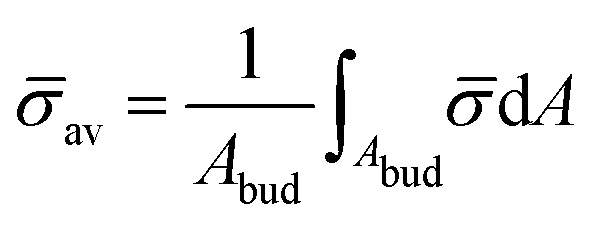 is the mean protein density on the bud, i.e. in the region above the membrane neck, and Abud is the area of the membrane comprised between s = 0 and the membrane neck. The vesicle size is now predicted to scale as rbud ∼ 1/(C0av). To test our scaling prediction we scale the bud radius rbud with C0av, which collapses the data onto a single line. To further illustrate the self-similar dynamics in the budding process, we rescale all lengths with the predicted bud size ∼1/(C0av) at the time tcut and shift the profiles so they all start at the same zmax at r = 0, see Fig. 8c–e. The upper part of the vesicle all follow the same spherical cap as we would expect from Fig. 8b, but interestingly the profiles map onto a universal shape also in the neck region (inner region) although the far field (outer region) is very different as it takes an Ω, pearl and flat shape. We zoom into the shedding vesicle and plot all the obtained membrane profiles together, which collapses onto a universal shape, shown in Fig. 8f. It is interesting to place this in the context of models for neck closure, where it was recently shown that there are optimal angles formed by the membrane depending on the outer membrane shape with a shape of a dome or a cone.80 In the model developed here neck constriction is achieved despite that there is no assembly of specialised scission proteins, but still reveal an optimal angle shared among all shapes Fig. 8f for all the rescaled data K1 ∈ [1.35–9], H0 ∈ [0.0015–0.15].
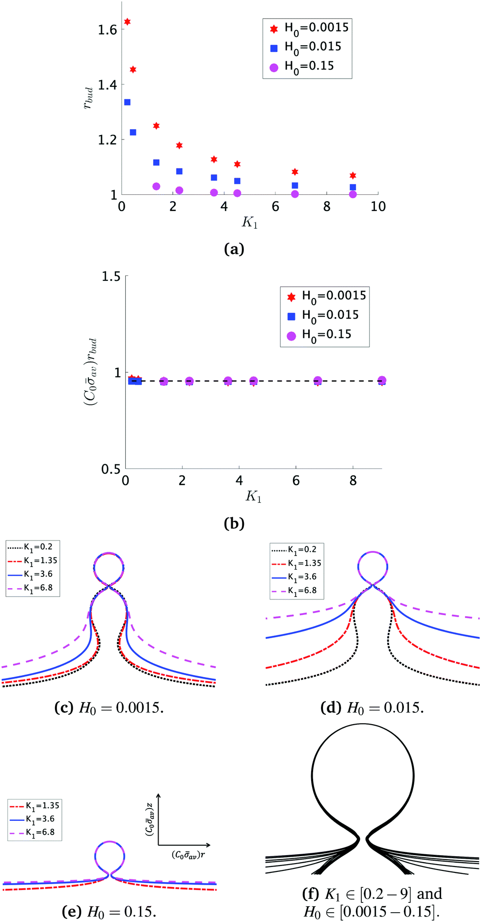 | ||
Fig. 8 (a) The bud radius rbud as a function of K1. For small values of H0, the vesicle size depends on the parameter K1: As K1 is smaller the vesicles have larger sizes, but as H0 increases this dependence becomes less significant, as it happens when H0 = 0.15. In this case, all the vesicles formed have nearly the same size, independent of K1. (b) We approximate the bud size as the inverse of the spontaneous curvature induced by the average concentration of proteins on the bud 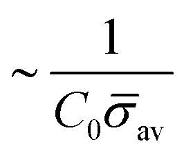 . The average protein density on the bud is computed as . The average protein density on the bud is computed as  . It is observed that all vesicle sizes shown in (a) collapse onto a single curve. The dashed straight line illustrates the average ratio (C0av)rbud. In figure (c)–(e) we plot the rescaled shapes at t = tcut for selected values of K1, when (c) H0 = 0.0015, (d) H0 = 0.015 and (e) H0 = 0.15. The radial coordinate r and the height z have been scaled with 1/(avC0) for each of the values of K1 and H0 considered. (c)–(e) Show that the upper part of the budding structures are very similar despite being connected to a membrane with very different shape (Ω, pearl, flat). In (f) we zoom into the vesicle and plot together all the obtained shapes at tcut. This reveals that in addition to the vesicle radius, the vesicle neck has almost the same shape regardless of K1 and H0. . It is observed that all vesicle sizes shown in (a) collapse onto a single curve. The dashed straight line illustrates the average ratio (C0av)rbud. In figure (c)–(e) we plot the rescaled shapes at t = tcut for selected values of K1, when (c) H0 = 0.0015, (d) H0 = 0.015 and (e) H0 = 0.15. The radial coordinate r and the height z have been scaled with 1/(avC0) for each of the values of K1 and H0 considered. (c)–(e) Show that the upper part of the budding structures are very similar despite being connected to a membrane with very different shape (Ω, pearl, flat). In (f) we zoom into the vesicle and plot together all the obtained shapes at tcut. This reveals that in addition to the vesicle radius, the vesicle neck has almost the same shape regardless of K1 and H0. | ||
4 Conclusions
We proposed a minimal mathematical model to describe the diffuso-kinetic membrane dynamics as curvature inducing proteins are recruited to a membrane and diffuse along its surface. The ratio of the diffusive and the kinetic time scale (K1) and the proteins sensitivity to mean curvature (H0) are systematically changed in our numerical simulations, which predicts a continuous formation of vesicles from a pearl-like membrane structure to the formation of a single vesicle from a nearly flat membrane. The coupled mechanism between diffusion and kinetic recruitment of proteins in the membrane leads to the formation of vesicles with narrow necks at the last stages of the membrane deformation, without the action of additional mechanisms or protein complexes that might be responsible for constriction of membrane vesicle necks. The budding time is found to follow a power-law tcut ∼ K1−2/3, despite varying the parameter H0 over a few orders of magnitude and of going from diffusion (K1 < 1) dominated to recruitment dominated (K1 > 1) dynamics.We derive a scaling law tcut ∼ K1−2/3 based on considering the interplay between the time scale associated with the diffusive spreading of the area allowing protein recruitment and the kinetically limited recruitment process associated with the increase of the local protein density in this area of the membrane. We extract the predicted vesicle size rbud that is a function of both K1 and H0, but asymptotes towards a constant vesicle size for K1 > 9 where it becomes insensitive to H0. We propose a scaling law for the vesicle size rbud ∼ 1/(C0av) based on the spontaneous curvature induced by the recruited proteins (C0av) where av is the mean protein density in the vesicle. By rescaling the numerical prediction for rbud with this scaling law collapses the data onto a single curve, further highlighting the self-similar budding dynamics.
The membrane shapes predicted by our minimal model can be found in a wide range of biological processes as well as induced by polymers and nanoparticle on lipid vesicles.18,81 The mathematical model couples the energy of the membrane to the diffuso-kinetics of the recruited proteins, providing a minimal description of the dynamics. Since the kinetic models describing protein recruitment are phenomenological, as details about the precise binding mechanisms of proteins are, to a large extent, missing in the field, we hope future work can closer couple these and incorporate the statistical mechanics properties as well as viscous flow effects in the recruitment dynamics of curvature sensing proteins. The model proposed here may form a basis for further characterizing how additional biophysical effects e.g., line tension, non-homogeneous bending rigidity and diffusion coefficient and direct protein–protein interactions influence the membrane dynamics.
Conflicts of interest
There are no conflicts to declare.Acknowledgements
R. R. M, S. L. and A. C. gratefully acknowledge funding from the Research Council of Norway, grant number 263056.Notes and references
- L.-G. Wu, E. Hamid, W. Shin and H.-C. Chiang, Annu. Rev. Physiol., 2014, 76, 301–331 CrossRef CAS.
- W. Weissenhorn, E. Poudevigne, G. Effantin and P. Bassereau, Curr. Opin. Virol., 2013, 3, 159–167 CrossRef CAS.
- J. H. Hurley and P. I. Hanson, Nat. Rev. Mol. Cell Biol., 2010, 11, 556–566 CrossRef CAS.
- A. F. Loftus, V. L. Hsieh and R. Parthasarathy, Biochem. Biophys. Res. Commun., 2012, 426, 585–589 CrossRef CAS.
- J. A. Dix and A. Verkman, Annu. Rev. Biophys., 2008, 37, 247–263 CrossRef CAS.
- A. Kenworthy, B. Nichols, C. Remmert, G. Hendrix, M. Kumar, J. Zimmerberg and J. Lippincott-Schwartz, J. Cell Biol., 2004, 165, 735–746 CrossRef CAS.
- N. Jouvenet, M. Zhadina, P. D. Bieniasz and S. M. Simon, Nat. Cell Biol., 2011, 13, 394–401 CrossRef CAS.
- E. M. Wenzel, S. W. Schultz, K. O. Schink, N. M. Pedersen, V. Nahse, A. Carlson, A. Brech, H. Stenmark and C. Raiborg, Nat. Commun., 2018, 9, 2932 CrossRef.
- T. Itoh, K. S. Erdmann, A. Roux, B. Habermann, H. Werner and P. de Camilli, Dev. Cell, 2005, 9, 791–804 CrossRef CAS.
- S. Boulant, C. Kural, J.-C. Zeeh, F. Ubelmann and T. Kirchhausen, Nat. Cell Biol., 2011, 13, 1124–1131 CrossRef CAS.
- L. Lanzetti, Curr. Opin. Cell Biol., 2007, 19, 453–458 CrossRef CAS.
- S. Liese, E. M. Wenzel, R. V. Rojas Molina, S. W. Schultz, H. Stenmark, C. Raiborg and A. Carlson, bioRxiv, 2019 DOI:10.1101/834457.
- M. G. Ford, I. G. Mills, B. J. Peter, Y. Vallis, G. J. Praefcke, P. R. Evans and H. T. McMahon, Nature, 2002, 419, 361–366 CrossRef CAS.
- F. Campelo, H. T. McMahon and M. M. Kozlov, Biophys. J., 2008, 95, 2325–2339 CrossRef CAS.
- P. D. Blood, R. D. Swenson and G. A. Voth, Biophys. J., 2008, 95, 1866–1876 CrossRef CAS.
- J. C. Stachowiak, C. C. Hayden and D. Y. Sasaki, Proc. Natl. Acad. Sci. U. S. A., 2010, 107, 7781–7786 CrossRef CAS.
- W. T. Snead, C. C. Hayden, A. K. Gadok, C. Zhao, E. M. Lafer, P. Rangamani and J. C. Stachowiak, Proc. Natl. Acad. Sci. U. S. A., 2017, 114, E3258–E3267 CrossRef CAS.
- I. Tsafrir, D. Sagi, T. Arzi, M. Guedeau-Boudeville, V. Frette, D. Kandel and J. Stavans, Phys. Rev. Lett., 2001, 86, 1138–1141 CrossRef CAS.
- J. C. Stachowiak, E. M. Schmid, C. J. Ryan, H. S. Ann, D. Y. Sasaki, M. B. Sherman, P. L. Geissler, D. A. Fletcher and C. C. Hayden, Nat. Cell Biol., 2012, 14, 944 CrossRef CAS.
- R. Dimova, Adv. Colloid Interface Sci., 2014, 208, 225–234 CrossRef CAS.
- I. Tsafrir, Y. Caspi, M.-A. Guedeau-Boudeville, T. Arzi and J. Stavans, Phys. Rev. Lett., 2003, 91, 138102 CrossRef.
- O. Avinoam, M. Schorb, C. J. Beese, J. A. G. Briggs and M. Kaksonen, Science, 2015, 348, 1369–1372 CrossRef CAS.
- H. McMahon and J. Gallop, Nature, 2005, 438, 590–596 CrossRef CAS.
- M. Kaksonen, C. Toret and D. Drubin, Cell, 2005, 123, 305–320 CrossRef CAS.
- M. Rosendale and D. Perrais, Int. J. Biochem. Cell Biol., 2017, 93, 41–45 CrossRef CAS.
- A. Agrawal and D. J. Steigmann, Z. Angew. Math. Phys., 2011, 62, 549–563 CrossRef CAS.
- J. Derganc, B. Antonny and A. Copic, Trends Biochem. Sci., 2013, 38, 576–584 CrossRef CAS.
- G. Guigas and M. Weiss, Biochim. Biophys. Acta, Biomembr., 2016, 1858, 2441–2450 CrossRef CAS.
- J. Derganc and A. Copic, Biochim. Biophys. Acta, Biomembr., 2016, 1858, 1152–1159 CrossRef CAS.
- W. T. Gozdz, J. Chem. Phys., 2011, 134, 024110 CrossRef CAS.
- R. Lipowsky, Faraday Discuss., 2013, 161, 305 RSC.
- P. Rangamani, K. K. Mandadap and G. Oster, Biophys. J., 2014, 107, 751–762 CrossRef CAS.
- C. Tozzi, N. Walani and M. Arroyo, New J. Phys., 2019, 21, 093004 CrossRef CAS.
- A. Mahapatra, D. Saintillan and P. Rangamani, bioRxiv, 2020 DOI:10.1101/2020.01.14.906917.
- J. S. Sohn, Y.-H. Tseng, S. Li, A. Voigt and J. S. Lowengrub, J. Comput. Phys., 2010, 229, 119–144 CrossRef CAS.
- J. Lowengrub, J. Allard and S. Aland, J. Comput. Phys., 2016, 309, 112–128 CrossRef CAS.
- K. E. Teigen, X. Li, J. Lowengrub, F. Wang and A. Voigt, Commun. Math. Sci., 2009, 7, 1009–1037 CrossRef.
- W. Helfrich, Z. Naturforsch., C: J. Biosci., 1973, 28, 693–703 CAS.
- P. B. Canham, J. Theor. Biol., 1970, 26, 61–81 CrossRef CAS.
- H. Deuling and W. Helfrich, Biophys. J., 1976, 16, 861–868 CrossRef CAS.
- H. Alimohamadi and P. Rangamani, Biomolecules, 2018, 8, 120 CrossRef.
- D. Schley, R. J. Whittaker and B. W. Neuman, J. R. Soc., Interface, 2013, 10, 20130403 CrossRef.
- S. Dmitrieff and F. Nedelec, PLoS Comput. Biol., 2015, 11, 1–15 CrossRef.
- L. Foret, Eur. Phys. J. E: Soft Matter Biol. Phys., 2014, 37, 42 CrossRef.
- H. Alimohamadi, B. Ovryn and P. Rangamani, Sci. Rep., 2020, 10, 1–15 CrossRef.
- M. Arroyo, N. Walani, A. Torres-Sánchez and D. Kaurin, Onsager's Variational Principle in Soft Matter: Introduction and Application to the Dynamics of Adsorption of Proteins onto Fluid Membranes, in The Role of Mechanics in the Study of Lipid Bilayers. CISM International Centre for Mechanical Sciences (Courses and Lectures), ed. D. Steigmann, Springer, Cham, 2018 Search PubMed.
- A. Torres-Sanchez, D. Millan and M. Arroyo, J. Fluid Mech., 2019, 872, 218–271 CrossRef CAS.
- N. S. Gov, Philos. Trans. R. Soc., B, 2018, 373, 20170115 CrossRef.
- A. Veksler and N. S. Gov, Biophys. J., 2007, 93, 3798–3810 CrossRef CAS.
- R. Lipowsky, Faraday Discuss., 2013, 161, 305–331 RSC.
- R. Lipowsky, Adv. Colloid Interface Sci., 2014, 208, 14–24 CrossRef CAS.
- C.-H. Chang and E. I. Franses, Colloids Surf., A, 1995, 100, 1–45 CrossRef CAS.
- K. Foo and B. Hameed, Chem. Eng. J., 2010, 156, 2–10 CrossRef CAS.
- S. Leibler, J. Phys., 1986, 47, 507–516 CrossRef CAS.
- H. Jian-Guo and O.-Y. Zhong-Can, Phys. Rev. E: Stat., Nonlinear, Soft Matter Phys., 1993, 47, 461–467 CrossRef.
- M. Deserno, Notes on differential geometry, 2004 Search PubMed.
- U. Seifert, K. Berndl and R. Lipowsky, Phys. Rev. A: At., Mol., Opt. Phys., 1991, 44, 1182–1202 CrossRef CAS.
- S. P. Preston, O. E. Jensen and G. Richardson, Q. J. Mech. Appl. Math., 2008, 61, 1–24 CrossRef.
- E. M. Smith, J. Hennen, Y. Chen and J. D. Mueller, Biophys. J., 2015, 108, 2648–2657 CrossRef CAS.
- P. M. Chaikin and T. C. Lubensky, Principles of condensed matter physics, Cambridge University Press, 1995 Search PubMed.
- G. B. Arfken, H. J. Weber and F. E. Harris, Mathematical methods for physicists, Academic Press, 7th edn, 2013 Search PubMed.
- T. Masuda, H. Hirose, K. Baba, A. Walrant, S. Sagan, N. Inagaki, T. Fujimoto and S. Futaki, Bioconjugate Chem., 2020, 31, 1611–1615 CrossRef CAS.
- J. B. Larsen, M. B. Jensen, V. K. Bhatia, S. L. Pedersen, T. Bjornholm, L. Iversen, M. J. Uline, I. Szleifer, K. J. Jensen, N. S. Hatzakis and D. Stamou, Nat. Chem. Biol., 2015, 11, 192–194 CrossRef CAS.
- W. Zhao, L. Hanson, H.-Y. Lou, M. Akamatsu, P. D. Chowdary, F. Santoro, J. R. Marks, A. Grassart, D. G. Drubin, Y. Cui and B. Cui, Nat. Nanotechnol., 2017, 12, 750–756 CrossRef CAS.
- C. Florentsen, A. Kamp-Sonne, G. Moreno-Pescador, W. Pezeshkian, A. A. H. Zanjani, H. Khandelia, J. Nylandsted and P. M. Bendix, Soft Matter, 2020 10.1039/d0sm00241k.
- T. V. S. Krishnan, S. L. Das and P. B. S. Kumar, Soft Matter, 2019, 15, 2071–2080 RSC.
- J. Liu, Y. Sun, D. G. Drubin and G. F. Oster, PLoS Biol., 2009, 7, 1–16 Search PubMed.
- P. A. Janmey and P. K. J. Kinnunen, Trends Cell Biol., 2006, 16, 538–546 CrossRef CAS.
- P. Cicuta, S. L. Keller and S. L. Veatch, J. Phys. Chem. B, 2007, 111, 3328–3331 CrossRef CAS.
- P. Sens, Phys. Rev. Lett., 2004, 93, 108103 CrossRef.
- A. Carlson and L. Mahadevan, PLoS Comput. Biol., 2015, 11, 1–16 CrossRef.
- D. Wirtz, Annu. Rev. Biophys., 2009, 38, 301–326 CrossRef CAS.
- J. Liu, R. Tourdot, V. Ramanan, N. J. Agrawal and R. Radhakrishanan, Mol. Phys., 2012, 110, 1127–1137 CrossRef CAS.
- Z. Shi and T. Baumgart, Nat. Commun., 2015, 6, 5974 CrossRef CAS.
- D. Thalmeier, J. Halatek and E. Frey, Proc. Natl. Acad. Sci. U. S. A., 2016, 113, 548–553 CrossRef CAS.
- J. Liu, Y. Sun, G. F. Oster and D. G. Drubin, Curr. Opin. Cell Biol., 2010, 22, 36–43 CrossRef CAS.
- M. M. Kozlov and L. V. Chernomordik, Curr. Opin. Struct. Biol., 2015, 33, 61–67 CrossRef CAS.
- P. G. Saffman and M. Delbrück, Proc. Natl. Acad. Sci. U. S. A., 1975, 72, 3111–3113 CrossRef CAS.
- P. Bassereau, R. Jin, T. Baumgart, M. Deserno, R. Dimova, V. A. Frolov, P. V. Bashkirov, H. Grubmueller, R. Jahn, H. J. Risselada, L. Johannes, M. M. Kozlov, R. Lipowsky, T. J. Pucadyil, W. F. Zeno, J. C. Stachowiak, D. Stamou, A. Breuer, L. Lauritsen, C. Simon, C. Sykes, G. A. Voth and T. R. Weikl, J. Phys. D: Appl. Phys., 2018, 51, 343001 CrossRef.
- J. Agudo-Canalejo and R. Lipowsky, PLoS Comput. Biol., 2018, 14, 1–21 CrossRef.
- Y. Yu and S. Granick, J. Am. Chem. Soc., 2009, 131, 14158–14159 CrossRef CAS.
Footnote |
| † Electronic supplementary information (ESI) available. See DOI: 10.1039/d0sm01028f |
| This journal is © The Royal Society of Chemistry 2020 |